Spatio-Temporal Modeling of COVID-19 Spread in Relation to Urban Land Uses: An Agent-Based Approach

Abstract

This study aims to address the existing gaps in evidence regarding spatio-temporal modeling of COVID-19 spread, specifically focusing on the impact of different urban land uses in a geospatial information system framework. It employs an agent-based model at the individual level in Gorgan, northeast Iran, characterized by diverse spatial and demographic features. The interactions between human agents and their environment were considered by incorporating social activities based on different urban land uses. The proposed model was integrated with the susceptible–asymptomatic–symptomatic–on treatment–aggravated infection–recovered–dead epidemic model to better understand the disease transmission at the micro-level. The effect of various intervention scenarios, such as social distancing, complete and partial lockdowns, restriction of social gatherings, and vaccination was investigated. The model was evaluated in three modes of cases, deaths, and the spatial distribution of COVID-19. The results show that the disease was more concentrated in central areas with a high population density and dense urban land use. The proposed model predicted the distribution of disease cases and mortality for different age groups, achieving 72% and 71% accuracy, respectively. Additionally, the model was able to predict the spatial distribution of disease cases at the neighborhood level with 86% accuracy. Moreover, findings demonstrated that early implementation of control scenarios, such as social distancing and vaccination, can effectively reduce the transmission of COVID-19 spread and control the epidemic. In conclusion, the proposed model can serve as a valuable tool for health policymakers and urban planners. This spatio-temporal model not only advances our understanding of COVID-19 dynamics but also provides practical tools for addressing future pandemics and urban health challenges.

1. Introduction

As of February 2023, the coronavirus (COVID-19) pandemic had adversely affected over 660 million people and had killed almost 6.7 million people worldwide [1]. The disease has become a major public health issue with unprecedented social and economic damages. Iran was identified as the second center of the pandemic after China [2], with a higher case fatality ratio (CFR) than the global average (CFR: 1.91% vs. 1.01%) as of 6 January 2023 [1]. Despite implementing various control measures, such as early testing, contact tracing, social distancing, and mass vaccination to control the outbreak, new waves of the disease continue to emerge [1].

Previous studies have demonstrated that combining a geographical information system (GIS) with spatial statistics or machine learning algorithms can provide a robust framework to explore the spatial patterns of infectious diseases [3,4]. For instance, Tabasi et al. [5] identified the spatio-temporal clusters of COVID-19 based on epidemiological features in Golestan province, Iran. They found that these clusters varied based on epidemiological characteristics with higher concentrations in areas with a higher proportion of young adults. In Bangladesh, Masrur et al. [6] investigated the spatial and temporal patterns of COVID-19 using space-time clustering techniques. Their results show that the central and southeastern regions have a higher risk of COVID-19 transmission and that the failure to comply with preventive public health measures could lead to the formation of larger disease clusters..

Even though the studies above provide useful insight about the spatial and temporal patterns of COVID-19 and influential factors, they lack the ability to examine the spread of the epidemic in an area with complex social structures, such as the spatial dynamics of the disease, and the effect of control strategies on the disease outbreak. To address this gap, several mathematical models have been applied to simulate the process of COVID-19 transmission and the effectiveness of control scenarios. Some of these attempts have used susceptible–infected–recovered (SIR) epidemic models [7,8,9] or more detailed simulations using susceptible–exposed–infected–recovered (SEIR) epidemic models [10,11]. While these approaches are useful to understand the general behavior of epidemics at large scales, they have limitations in accurately modeling the spatial spread of a disease at the micro-level, such as individual-based behaviors and interactions between individuals, as they assume that all individuals in a diseased state (e.g., infected) have similar characteristics.

Unlike the classic mathematical models, in agent-based models (ABMs), dynamic interactions between agents and the environment are simulated in a heterogeneous population, allowing various agents in the same conditions to make different decisions based on their characteristics and experiences [12]. ABMs offer a unique framework for exploring diverse views of disease dynamics at the individual level and investigating how demographic factors such as age can affect the disease outbreak [13,14]. ABMs include agents with a set of properties known as units of modeling, an environment, and a set of rules to govern their behaviors. Moreover, the influence of the system on individual behaviors and the influence of these behaviors on the system are examined; therefore, complex behaviors at higher levels are the result of collective interactions of agents at lower levels [15]. Recently, several ABMs were developed to model COVID-19 transmission. Bouchnita and Jebrane [16] developed a multi-scale hybrid ABM to evaluate the effect of control measures on the spread of COVID-19. They showed that even with social distancing measures in place, fear of the pandemic could make people more susceptible to infection, and the presence of asymptomatic cases could contribute to the exponential growth of the epidemic. Zhou et al. [17] examined the spatial heterogeneity of the COVID-19 outbreak and optimized the spatial allocation of vaccination efforts. They showed that herd immunity is heterogeneously distributed; therefore, vaccination strategies should be spatialized. However, their model did not take into account land use affecting the disease spread (e.g., educational and medical land use) and only considered four epidemic states (SEIR model) for human agents.

Integrating an ABM with the GIS can lead to a better understanding of the complex process of the spatio-temporal spread of diseases [18]. To our knowledge, there has been insufficient research on spatio-temporal modeling of the spread of COVID-19 using ABMs and the GIS at the individual level. Mahdizadeh Gharakhanlou and Hooshangi [19] simulated the spatio-temporal spread of COVID-19 using an ABM and susceptible–exposed–infected–recovered–dead (SEIRD) model in Urmia, Iran. They showed that closing educational facilities, heeding social distancing, and limiting the presence of civil servants in administrative centers could mitigate the severity of the disease. Olszewski et al. [20] analyzed the spatio-temporal spread of COVID-19 using an ABM. The results indicate that applying social restrictions resulted in a sharp reduction in COVID-19 incidence and flattened the epidemic waves.

To bridge the gap described above, this study aims to:

• Develop an ABM by integrating with an improved susceptible–asymptomatic–symptomatic–on treatment–aggravated infection–recovered–dead (SASOARD) model in the GIS framework to simulate the spatio-temporal spread of COVID-19.
• Incorporate the heterogeneous interactions within the community in the model.
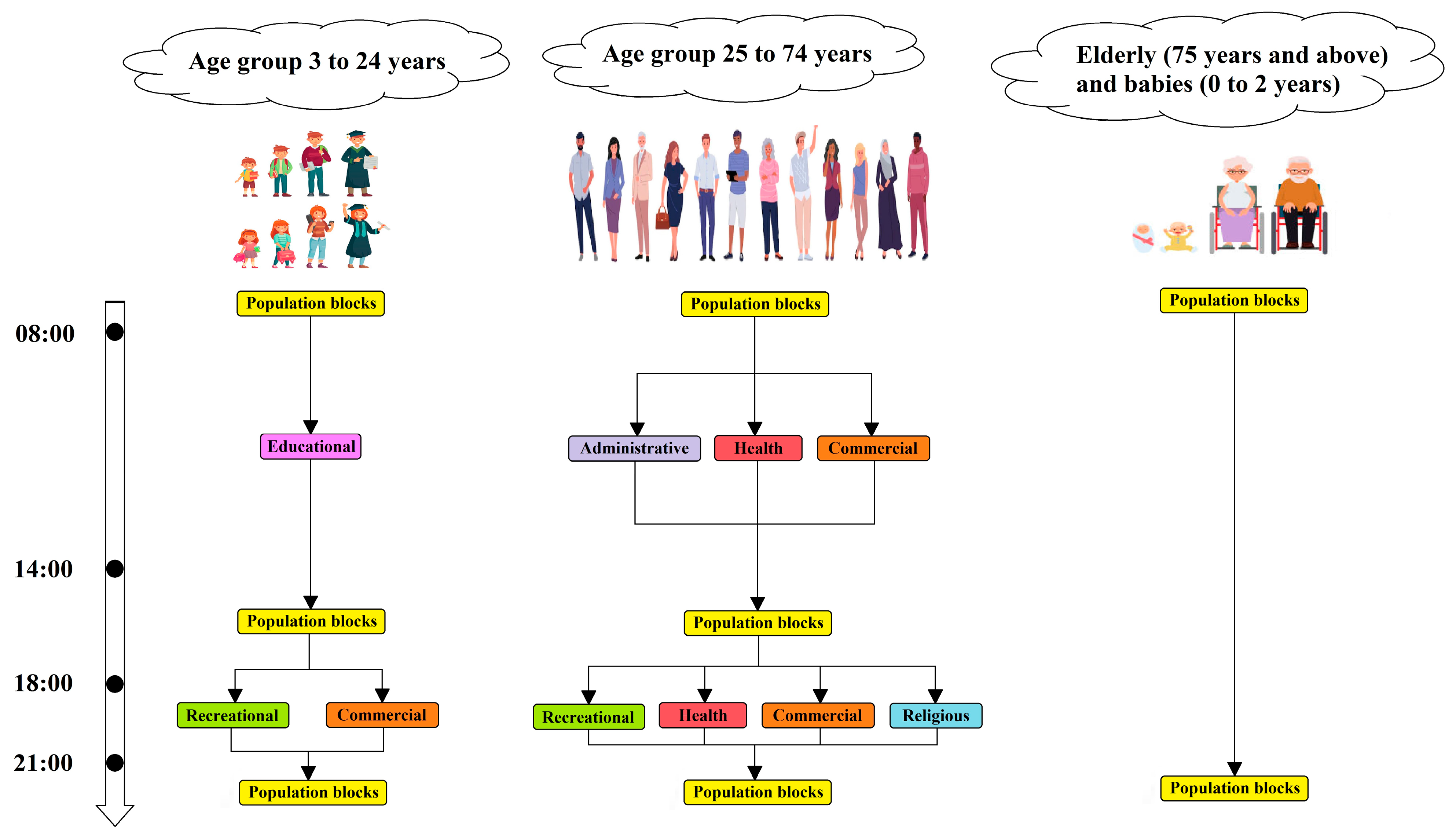
• Design the proposed model based on demographic data and different types of urban land use to track the spatial location of agents, their mobility, and the spatial spread of the disease.
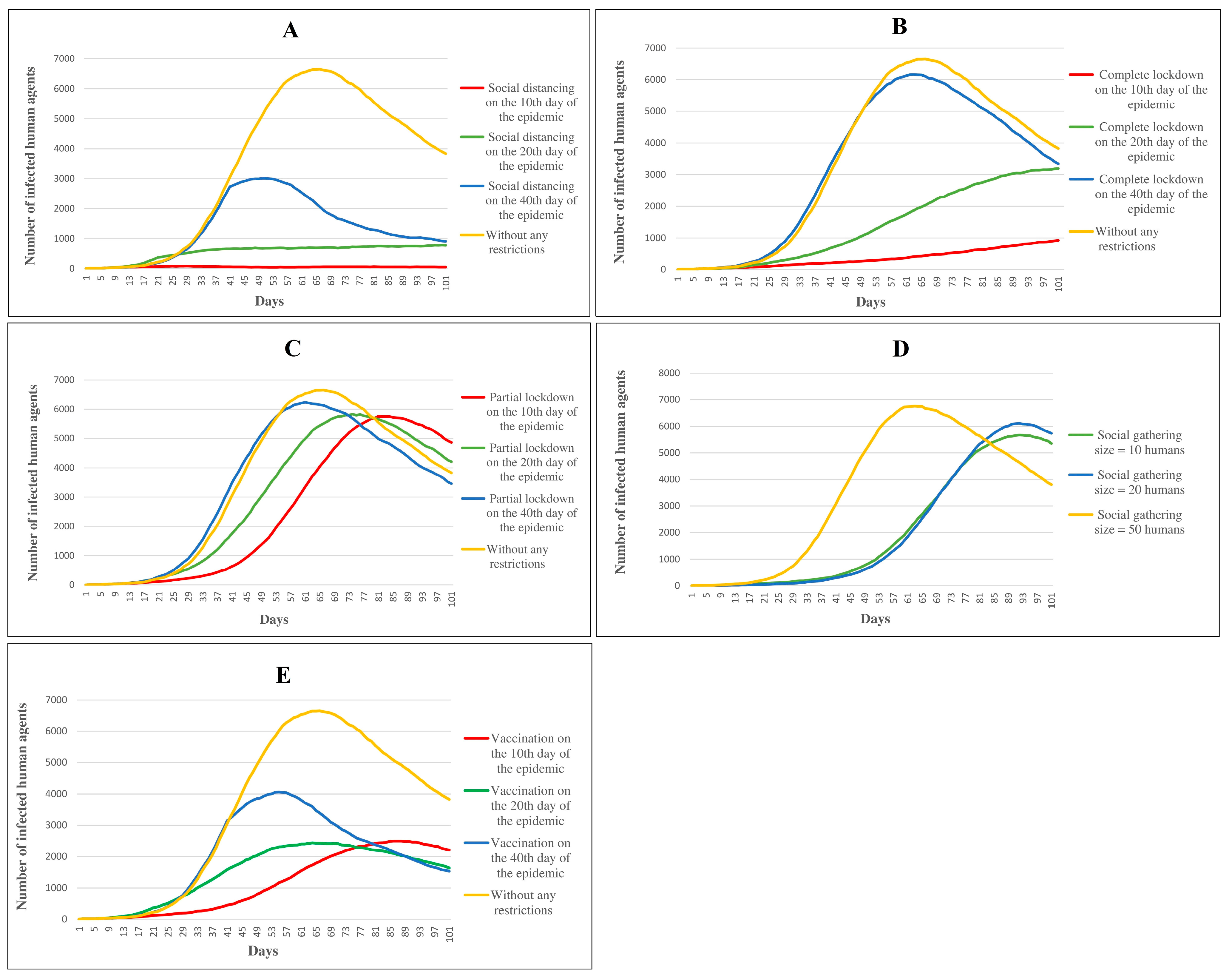
• Evaluate the effects of various intervention scenarios, including complete lockdown, partial lockdown, social distancing, restriction on social gatherings, and vaccination.
• Investigate the effect of urban land use on the COVID-19 outbreak.
• Identify vulnerable populations and disease-prone areas, which should be prioritized for more targeted and effective policies.

The proposed model can serve as a valuable tool to assist health policymakers to better understand the spatio-temporal spread of various strains of COVID-19 and evaluate the effective preventive measures. Moreover, the proposed ABM with GIS integration can be used as a spatial decision-support tool to promote urban resilience in the face of future pandemics.

2. Materials and Methods

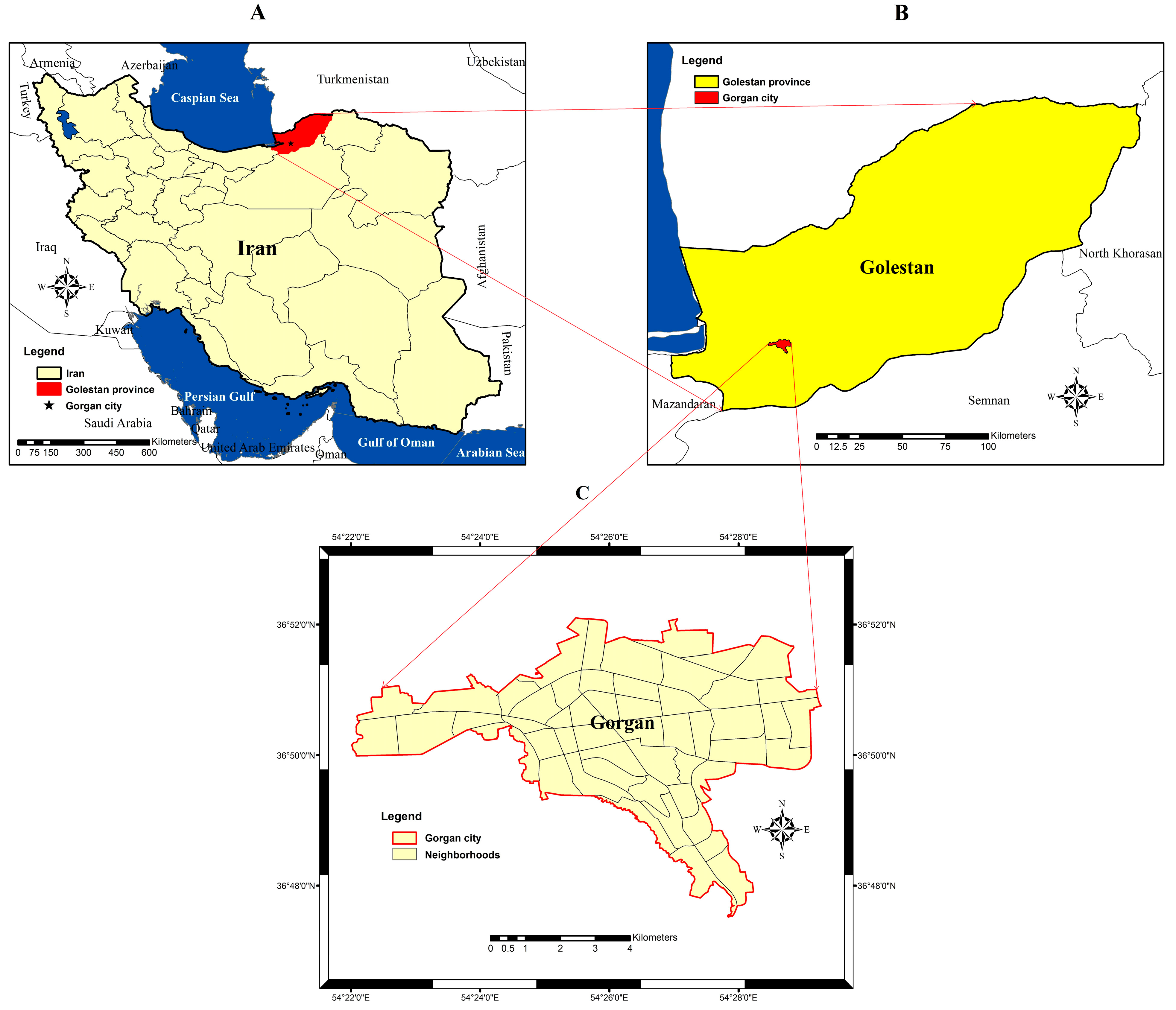
2.1. Study Area

The COVID-19 spread in Gorgan, the capital of Golestan province, which was one of the most vulnerable provinces of Iran to the disease in the first year of the pandemic [21], was modeled. The CFR in this province was reported to be about 2.5 times higher than the average CFR in Iran [1]. Gorgan has a very high population density, heterogeneous population characteristics, and ample urban facilities compared to other areas in this province (Figure 1). With a population of about 350,000 people, Gorgan is the most populous city in the province and consists of 52 neighborhoods and 1911 blocks [22]. Densely populated communities and high-density urban land use can increase the likelihood of COVID-19 transmission and make it an ideal location to study the spatial dynamics of the disease and evaluate the effectiveness of various intervention strategies [23].

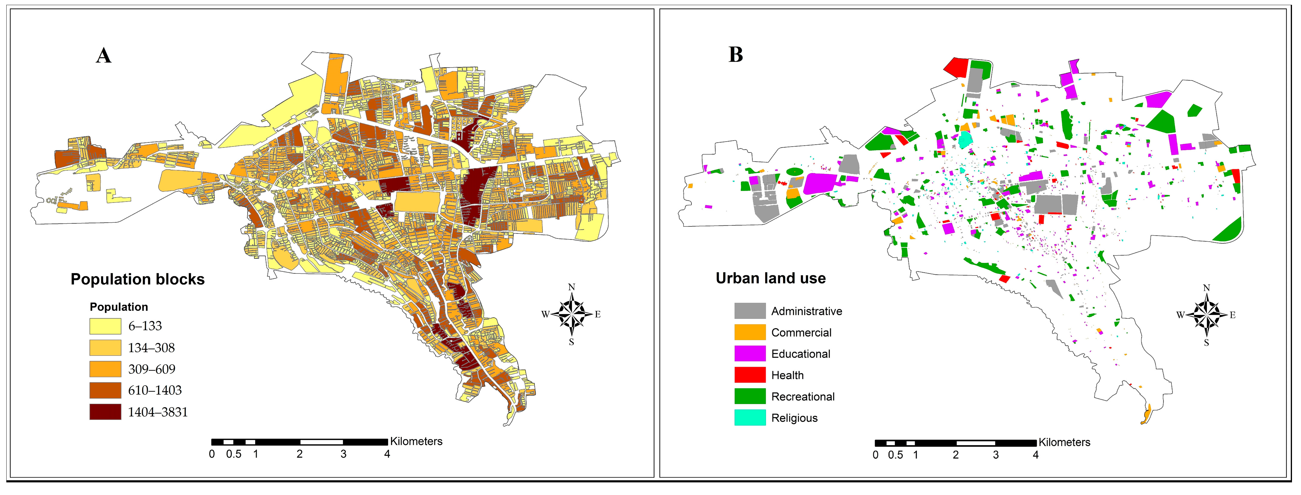
2.2. Data Collection and Preparation

A database of patient characteristics, demographic information, and spatial data was compiled. The database includes the confirmed COVID-19 cases in Gorgan from the beginning of the epidemic (1 February 2020) to 28 February 2021. For each patient who was either hospitalized due to the virus or tested positive, several characteristics, such as age, sex, date of diagnosis (or date of death due to treatment failure), and residential location, were retrieved from the Golestan province Center for Disease Control and Prevention (CDC) [21]. Demographic data on the number of residents in each block (Figure 2A), classified into 16 age groups ranging from 0–4 to 75+, were obtained from the Deputy of Statistics and Information of Golestan province [22].

Unlike previous studies that assumed a uniform distribution of the population, the actual distribution of the population was incorporated in the model [16,24,25,26]. The spatial data contains the spatial administrative boundary of the study area, population blocks, urban land use, and neighborhoods retrieved from the Deputy of Statistics and Information of Golestan province [22]. The land use maps include commercial, recreational, educational, administrative, health, and religious land use (Figure 2B).

The finest available scale for the disease data was the neighborhood level; therefore, the disease data (reported COVID-19 cases and deaths) were assigned to the corresponding neighborhood based on the patient’s address. Moreover, the demographic information was assigned to the corresponding block for all 16 age groups, allowing the actual population of each block to be assigned based on the age group. The disease and spatial data were prepared in Microsoft Excel 2016 and ArcGIS version 10.2 (ESRI, Redlands, CA, USA), respectively.

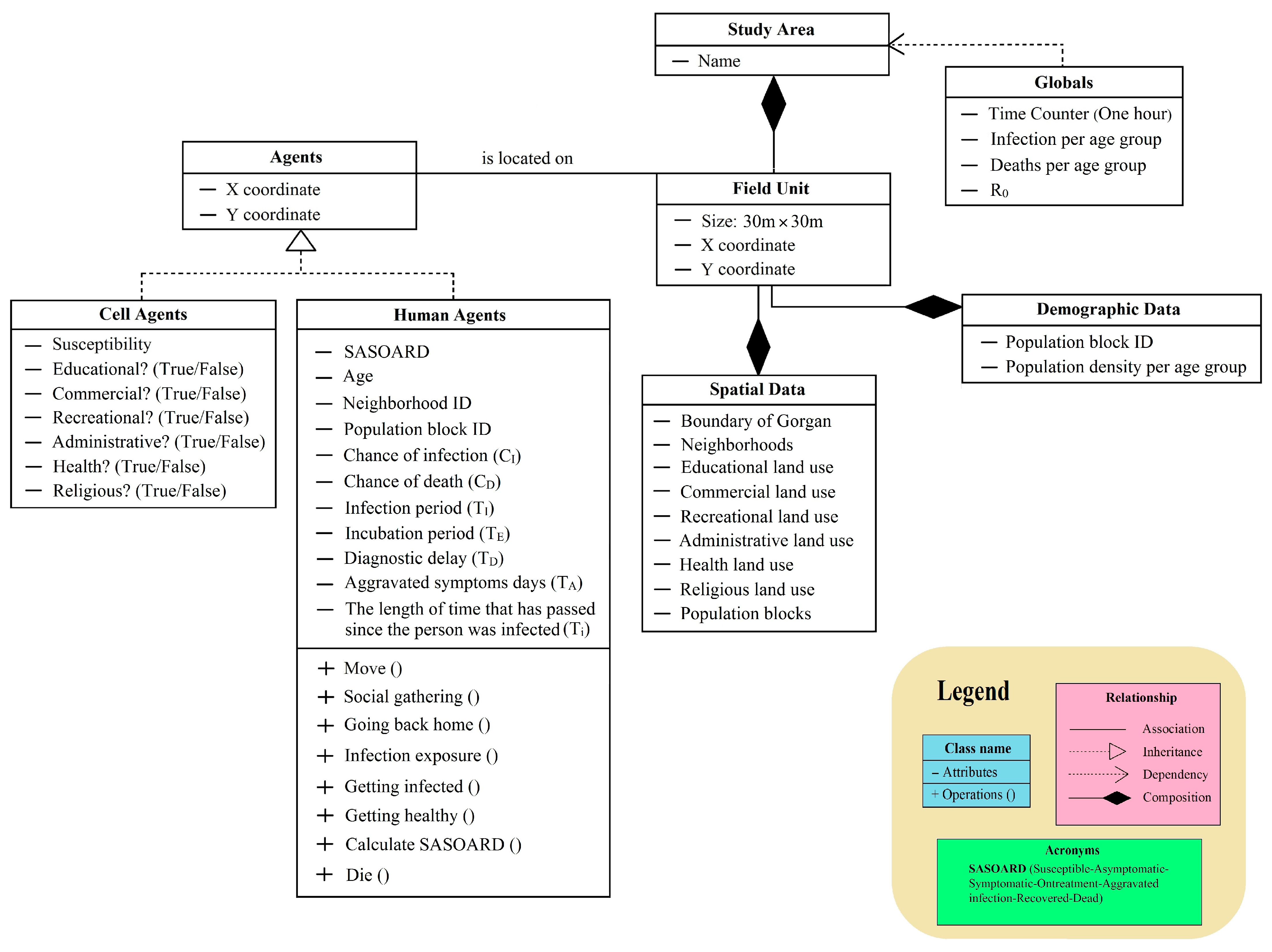
2.3. Model Development

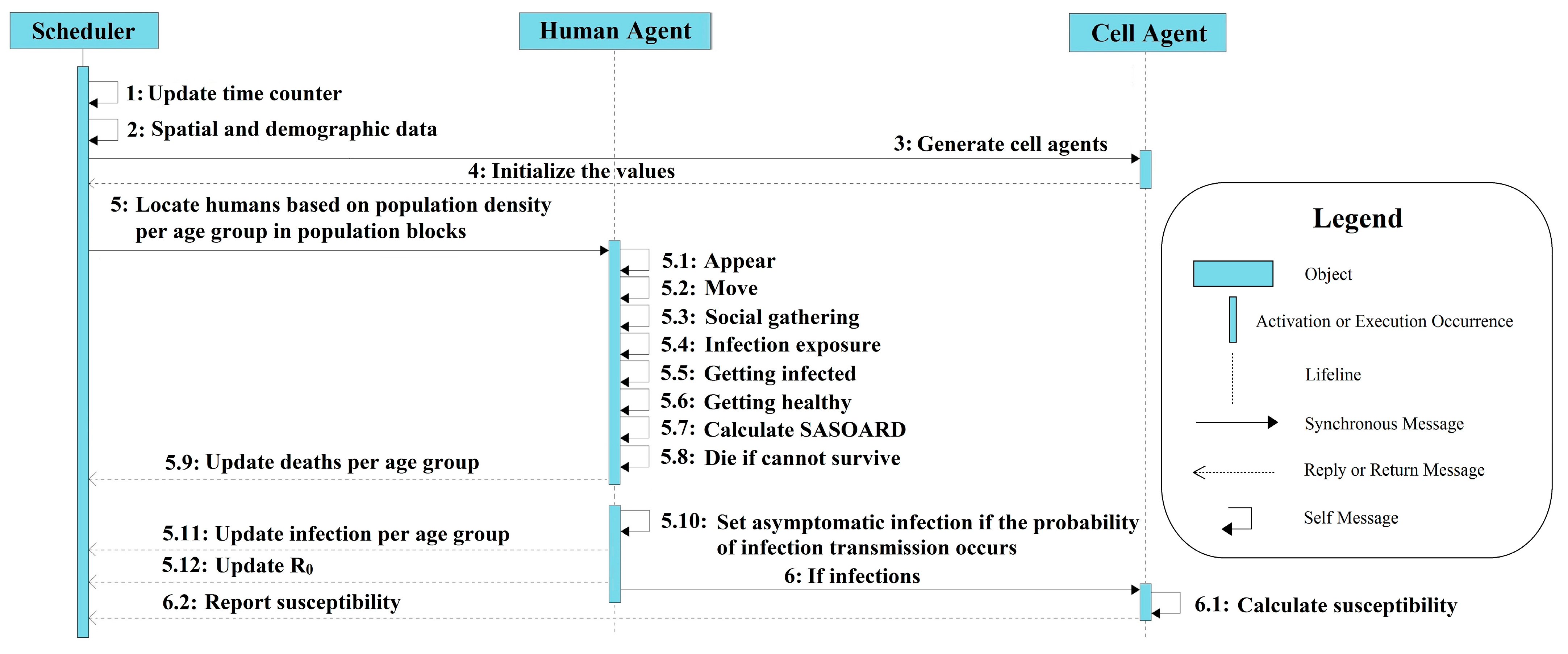
The overview, design concepts, and details (ODD) protocol was used to develop the ABM of COVID-19 transmission in Gorgan. The model begins with an overview of the processes and components involved. Then, the design concepts for the model are presented. Finally, the details of the model implementation are introduced. The model algorithms were executed in NetLogo programming language version 6.1.1 (Northwestern University, Evanston, IL, USA). The results were presented in the form of diagrams and maps in Microsoft Excel and ArcGIS Desktop, respectively.

2.3.1. Overview

The proposed model consists of two types of agents: human agents and cell agents. Each human agent has different characteristics and behaviors, and their likelihood of contracting or dying from COVID-19 varies based on their age group. The cell agents represent different land use in the studied area. The model assumes that COVID-19 is transmitted only between human agents and ignores the transmission of the disease in closed environments (e.g., through contaminated surfaces). A time step of one hour was considered in the model to account for transmission occurring at any time of the day; therefore, the proposed model can depict various interactions between human and cell agents in different time steps. The components of the proposed model are illustrated in the unified modeling language (UML) diagram (Figure 3).

All the processes performed by the agents in the proposed model in a time step and the relations between the processes are shown in Figure 4. More information about the model description are included in File S1 (Supplementary Materials).

2.3.2. Design Concepts

The main features that distinguish ABMs from other classical computational models are observability, randomness, interactions, and perception [18]. In each time step, specific observations can be tracked, including the number of infected, recovered, and deceased humans in each age group, the basic reproductive number (R₀), and the susceptibility of cell agents in each type of urban land use.

Regarding randomness, when a human agent (based on the age group) moves to the nearest land use relative to the distance from its population block, the location of that agent is randomly placed in one of the determined land use cells they visit. In addition, since adherence to social distancing in communities is not uniform [27], it is assumed that agents do not adhere to social distancing guidelines uniformly (as described in Section Social Distancing).

Disorganized interaction between agents is another main feature of the model. Cell agents with different characteristics (various land uses) attract different human agents (in terms of age group). Disease transmission between human agents also takes place in the environment (cell agents). These interactions can occur anywhere in the environment, at any time step, and can change according to different conditions. For example, human agents in the age group of 15 to 18 years move toward areas of educational land use (high schools) within a specific time limit (8 am to 2 pm), while in another time frame (6 pm to 9 pm), these agents visit areas of recreational and commercial land use; therefore, we are likely to observe heterogeneous spatial and temporal interactions.

Human agents participate in daily activities based on their perception of their health status. For example, if human agent sense disease symptoms, they quarantine themselves and do not participate in social activities. In addition, an infected human agent seeks medical services. If there is a capacity for hospital beds, this agent enters the ‘on-treatment’ stage. The cell agents (environment) can also perceive interactions between human agents. In other words, if the disease is transmitted between human agents, the cell agent related to the infected human realizes this condition and modifies its susceptibility.

2.3.3. Details

Many variables were incorporated into the ABM of COVID-19 transmission (

Table 1. A summary of the variables related to the ABM of the COVID-19 spread in the study area.

Variable	Description	Values	Source
Contagion days (TC)	No. of days it takes for infected people to be contagious, and the virus can spread from them to others	4 days	[2]
Contagion distance (DC)	Maximum distance for possible contagion	2 m	[28]
Infection period (TI)	The time interval between exposure to the virus and immunity to the virus	N(26,5) a days	[29]
Incubation period (TE)	The time interval between exposure to the virus and symptom onset	N(10,4) a days	[2]
Diagnostic delay (TD)	The time interval between the onset of symptoms and confirmed diagnosis of the disease	R(0,24) b hours	[21]
Aggravated symptoms days (TA)	The time interval between exposure to the virus and the onset of aggravated symptoms	TI divided by 2.5	[21]
Chance of aggravated infection (CA)	The probability that the acute stages of the disease will be seen in the infected person	18.5%	[21]
Mortality multiplier	The multiplying factor for the chance of death in the infected person	1 or 2 (1: when the aggravated symptoms are not seen in the infected person, 2: when the infected person has entered the aggravated infection stage)	[21]
Medical care capacity	The capacity of hospital beds in the study area	24.7 beds per 10 thousand people	[22]
Chance of infection (CI)	The probability of disease exposure for each age group	Minimum 0.07% (age group 5–9) and maximum 6.44% (age group 75 and above)	[21]
Chance of death (CD)	The probability of death for each age group	Minimum 1.18% (age group 25–29) and maximum 30.91% (age group 75 and above)	[21]

^a: The notation N(μ,σ), where N indicates that the distribution is normal, μ is the mean of the distribution, and σ is the standard deviation of the distribution. ^b: The notation R generates a random number in the interval (a,b).

). The model included key processes, such as human mobility, social gatherings, disease transmission, the SASOARD model, and the susceptibility map. In addition, various scenarios have been considered, such as social distancing, complete lockdown, partial lockdown, restriction in social gatherings, and vaccination.

Human Mobility

In this model, it is assumed that if the complete lockdown scenario is not activated, human agents who are not receiving treatment can move up to 30 m in any direction (randomly between 0 and 360°) within the environment during a specific time of the day (6 a.m. to 2 p.m.) based on the Moore neighborhood (a two-dimensional square lattice containing a central cell and the eight surrounding cells [30]); however, under the complete lockdown scenario, human agents are limited to move up to 3 m in any direction per time step (within the timeframe listed above). It should be noted that human agents cannot enter or exit the environment during the modeling process.

Social Gatherings

Inspired by the CovaSim framework [31], this study used a hybrid contact network for interaction between human agents. Since the data requirements (e.g., household, school, workplace, and community age mixing patterns; school size distributions, enrollment rates by age, student–teacher ratios; workplace size distributions, employment rates by age) could not be met in the study area, the SynthPops contact network, which has been applied in the CovaSim framework [31], was not used; therefore, the daily activity of human agents was scheduled in the model (Figure 5). This process is activated when partial and complete lockdown scenarios are not in effect. For example, human agents aged 3 to 24 years old attend the nearest educational land use from their population block at 8 am and remain there until 2 pm. Based on the age group, these agents attend kindergarten (aged 3–7 years old), elementary school (aged 7–11 years old), middle school (aged 12–14 years old), high school (aged 15–18 years old), or university (aged 19–24 years old). They return to their population blocks at 2 pm and stay there until 6 pm. Then, they go to the closest recreational and commercial land use and remain there until 9 pm. They return to their assigned population blocks at 9 pm and remain there until 8 am. The same activities will be repeated the next day. In the same way, human agents aged 25 to 74 years old go to certain areas of land use at specific times of the day, as shown in Figure 5. The process of social gatherings is inactive for human agents > 75 years old or <2 years old. It is assumed that the maximum gathering size is 50 people for each urban land use. For example, no more than 50 people can visit a gym (recreational land use) between 6 pm and 9 pm.

Disease Transmission

It is assumed that the process of disease transmission between human agents occurs only from 6 am to 12 am. The transmission process depends on various conditions, and if all are met, the disease will be transmitted. First, a susceptible human who is not on treatment must be within D_C (Table 1) of at least one infected human who has been infected during the last 4 days (T_C, Table 1). If the conditions are met, the susceptible human may become infected based on the probability of infection that varies per age group (Table 1). D_C is limited to a maximum of two meters and is defined based on the Moore neighborhood [30]. If the susceptible human becomes infected, the R₀ is updated, and the susceptibility of the cell where the infected human is located increases by one unit.

SASOARD Model

The SASOARD model considers different health states of human agents, which are determined based on their characteristics and the conditions encountered during the simulation. When a susceptible human is infected with the virus, he/she enters an asymptomatic status. After passing T_E and T_D (Table 1), the status changes to symptomatic. Symptomatic individuals do not participate in social activities. If a hospital bed is available, their status will change to the on-treatment status, meaning they no longer infect anyone, participate in social activities, and move within the environment. In addition, the probability of death is reduced by half. After passing the T_A, an infected human may enter the aggravated infection status based on a certain probability (C_A), and the likelihood of death for an aggravated infected human is doubled (Table 1). As the T_I passes (Table 1), the infected human recovers. If the recovered human has used a hospital bed, one unit is added to the available capacity of hospital beds. It is assumed that the recovered human will be immune to the virus during the simulation. From the onset of aggravated symptoms to the end of the T_I, the infected human may die from the virus based on certain probabilities (Table 1). At this stage, if this human has used medical services, the existing capacity of hospital beds in the model is increased by one unit.

Susceptibility Map

The susceptibility maps are generated to display the spatial spread of the disease. When a susceptible human becomes infected, the susceptibility of the cell agent in which that human is located increases by one unit. As the cell agents change at each time step, the disease susceptibility map is updated. Areas (cell agents) with higher susceptibility values indicate high-risk areas of the COVID-19 outbreak and are determined based on different types of urban land use (Figure 3).

Social Distancing

In this model, it is assumed that human agents do not uniformly adhere to this policy. When the scenario is activated, a random number (people’s adherence to this control scenario) between 0 and 2 m is added to the distance between the susceptible and infected humans, leading to decline in the disease transmission between human agents.

Complete Lockdown

When the complete lockdown scenario is implemented, human agents will not participate in any social activities, and their mobility within the environment will be restricted. In other words, human agents can only move up to 3 m at each time step and are required to return to their population block.

Partial Lockdown

When this scenario is activated, human agents will no longer be able to participate in social activities except for visiting areas of health land use; however, unlike the complete lockdown policy, the mobility of human agents is not restricted, and they can move within the environment, as described in the human mobility process (Section Human Mobility).

Restriction in Social Gatherings

One of the primary actions to mitigate disease transmission in communities is restrictions on social gatherings. As explained in Section Social Gatherings, it is assumed that a social gathering size would be a maximum of 50 individuals; thus, it is assumed that this restriction is in the form of reducing the gathering size for human agents.

Vaccination

Evidence indicates mass vaccination is the most effective way to combat the COVID-19 pandemic [32]; however, vaccination is only required for people without symptoms of the disease, otherwise, it aggravates the symptoms [32]. Thus, it is assumed that only susceptible human agents who have not yet been infected could be vaccinated. In this model, the vaccinated human agents will no longer contract the disease.

2.4. Model Verification

To verify the accuracy of the conceptual models and simulations, and to avoid logical errors in the translation of the model into code, model verification was performed [33]. This involved code walk-throughs, debugging, and verifying the model’s behavior by varying key parameters, such as T_E, T_I, and the initial infected population, while keeping other parameters of the model constant. To investigate the effect of the T_I on the epidemic process, the disease spread was examined using different values of T_I (13, 26, and 52 days). Next, the disease prevalence was investigated according to different values of T_E (5, 10, and 20 days). Then, the epidemic status under different initial infected population sizes (i.e., 0.02%, 0.2%, and 2% infected human agents of the total population) was examined, as explained in Section 3.2.

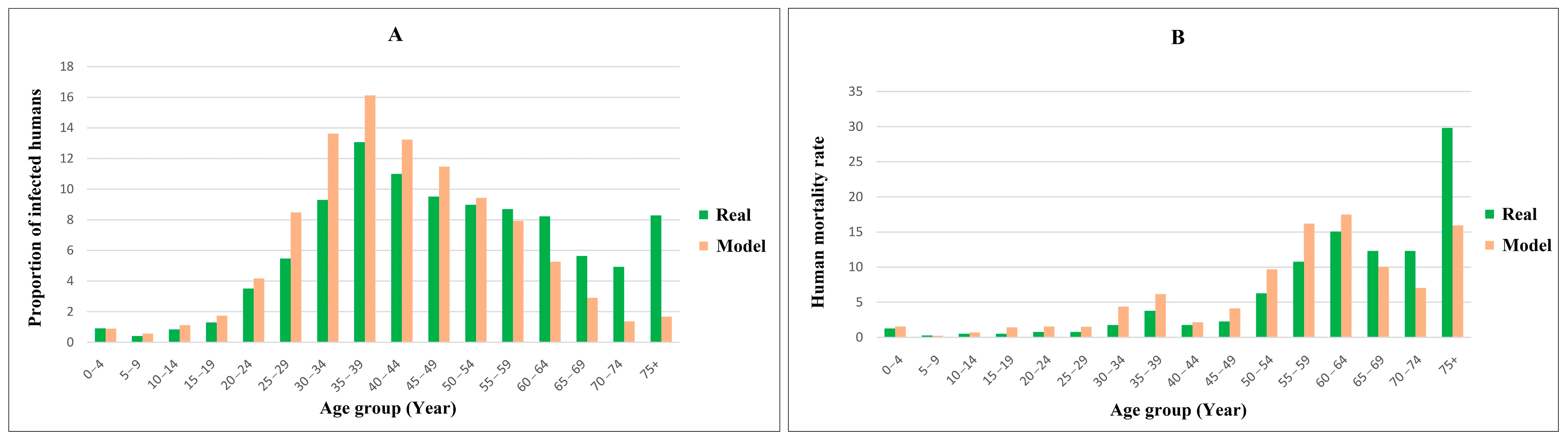
2.5. Model Validation

To confirm that the proposed model is a logical representation of reality, model validation was executed [33]. The proposed model was evaluated in terms of COVID-19 cases and deaths in different age groups and the spatial distribution of COVID-19 cases. The proportion of infected human agents in each age group to the total infected human agents (as a percentage) in the model was validated using actual values. Then, the proportion of deaths in each age group to the total number of deaths (as a percentage) in the model was compared with its corresponding observed values. To evaluate the spatial spread of COVID-19, the spatial distribution of the cases in 52 neighborhoods of the studied area in two modes of modeling and reality (disease data) was compared.

The coefficient of determination (R²) indicator was used to examine the model’s predictability [3]. The closer R² is to 1, the closer the predicted values by the model are to the observed values. Moreover, the Chi-square test was employed to examine the similarity of two data sets (e.g., predicted and observed values) based on Equation (1):

$${\mathsf{\chi }}^2={\sum }_{i=1}^n\frac{\left(Pi-Oi\right)²}{Oi}$$

(1)

where χ² represents the Chi-square value, Pi is the predicted value, and Oi is the observed value. For example, in this study, P₁ means the ratio of predicted COVID-19 cases in the age group of 0–4 years to the total predicted COVID-19 cases, and O₁ shows the proportion of observed COVID-19 cases in that age group to the total observed COVID-19 cases. In addition, i represents the number of situations in which the predicted and observed values can be compared; therefore, the value of i for COVID-19 cases and deaths in different age groups is 16, and its value for the spatial spread of COVID-19 in neighborhoods of the studied area is 52 (the number of neighborhoods). It should be noted that the model outputs in each condition have been obtained from the average of 100 simulations to account for variations and ensure the robustness of the results. The variance of the results was determined using Student’s t test with two-tailed confidence intervals and a significance level of 95%.

To identify the statistically significant hot and cold spots of the simulated COVID-19 outbreak, the optimized hot spot analysis was applied [34]. In addition, to compare the spatial directional distribution (i.e., central tendency and directional trend) of the simulated COVID-19 outbreak and the urban land use across the study area, the directional distribution (standard deviational ellipse) statistic was used [35]. Using the standard deviation ellipse (SDE), it is possible to determine whether the spatial distribution of the COVID-19 spread and the urban land use are elongated and therefore have a specific direction [35]. More information about the optimized hot spot and the directional distribution statistics is provided in [34,35].

The endemic equilibrium phase was also presented by using R₀. A disease reaches its endemic equilibrium state when the R₀ is greater than or equal to one during an epidemic [36]. To visualize the simulated epidemic trends and compare them with reality, we illustrated the weekly new cases (reported in reality) alongside the weekly R₀ (derived from the model) during the 14 weeks of the epidemic (from the beginning of the epidemic).

3. Results

3.1. Control Scenarios

As shown in Figure 6A, applying a social distancing scenario at different stages of the epidemic can result in various epidemic patterns. If this scenario is implemented on the 10th day, it is almost possible to control the epidemic; however, applying social distancing on the 20th and 40th days led to a significant reduction in disease cases (less than 1000 individuals after 100 days) compared to no social distancing restrictions.

As depicted in Figure 6B, applying the complete lockdown scenario on the 10th day of the epidemic led the epidemic peak to decrease by about 2000 units compared to its peak on the 20th day; however, if this scenario is applied on the 40th day of the epidemic, it has a limited effect in controlling the outbreak.

Figure 6C illustrates the results of a partial lockdown scenario at different times of the epidemic (the same as the social distancing scenario). Applying this scenario on the 10th day of the epidemic instead of applying it on the 20th day of the epidemic will lead to a delay in the peak of the epidemic by approximately 10 days and a slight reduction in the disease cases. In addition, applying this scenario on the 40th day of the epidemic has a limited effect in reducing disease cases.

The effect of different social gatherings sizes (10, 20, and 50 humans) on the disease spread was also examined. According to Figure 6D, reducing the size of the social gatherings leads to a decrease in the epidemic peak.

To assess the effect of population vaccination on the spread of the disease, it is assumed that 50% of the susceptible population is vaccinated on different days of the epidemic. As shown in Figure 6E, population vaccination has a potential effect in reducing disease outbreaks. If the vaccination is administered on the 10th day of the epidemic, it will result in a sharp reduction in the epidemic peak (roughly 60%) and a delay in its occurrence; however, when comparing the vaccination on the 10th and 20th days of the epidemic, there is no noticeable change in the peak of the epidemic, only a delay in its timing.

3.2. Model Verification

Figure 7 provides an illustration of the epidemic over time based on different scenarios for T_I, T_E, and the initial infected population. Figure 7A shows the disease spread using different values of T_I (13, 26, and 52 days) while keeping the other parameters of the model constant. The results indicate that as the T_I increases, the number of infected human agents also increases. A longer T_I results in a delayed epidemic peak and with a higher prevalence. The maximum number of infected human agents under the scenario of 52 days was almost 12,000, whereas for the 26- and 13-day scenarios, they were approximately 6000 and 3000, respectively; therefore, doubling the length of the T_I leads to double the number of COVID-19 cases at the epidemic peak.

Figure 7B displays the disease spread using different values of T_E (5, 10, and 20 days), with the other parameters held constant. As the T_E increases, the epidemic’s peak appears earlier (Figure 7B). Reducing the T_E from 20 to 10 days results in the epidemic peak occurring roughly 10 days later and infecting almost 6700 individuals; however, a further reduction in the T_E to 5 days lead to a significant delay in the epidemic peak.

Figure 7C illustrates the effect of the initial infected population on the epidemic under different population sizes (i.e., 0.02%, 0.2%, and 2% infected human agents of the total population). As the initial infected population increases from 0.02% to 0.2% and then to 2%, the epidemic peak occurs earlier, from 69 days to 53 days and then to 37 days, respectively. This implies that when the initial infected population is increased tenfold, the disease peak occurs roughly 15 days earlier; however, the increase in initial infected population only accelerates the epidemic peak and has no significant effect on the overall severity of the disease (Figure 7C).

3.3. Model Validation

Figure 8 displays the results of validating the model by comparing the proportion of infected human agents and the death rate with actual data. According to Figure 8A, the predicted proportion of infected humans in different age groups is similar to their corresponding observed values, indicating a good performance of the model (R² = 0.7198, (95% confidence interval (CI), 0.7060 to 0.7337)). In addition, the Chi-square value for the predicted and observed cases was calculated as 16, which was lower than the critical value (χ² _0.05 (15) = 24.996), meaning the null hypothesis is not rejected; therefore, there is no significant difference between the predicted and observed proportions in different age groups.

According to Figure 8B, the predicted mortality rates in different age groups were almost consistent with the corresponding observed values. The R² index indicates that the proposed model can predict the mortality pattern according to the age group with an accuracy of approximately 71% (R² = 0.7143, (95% CI, 0.6908 to 0.7379)). The calculated value for the Chi-square test (χ² = 24.498) was lower than the critical value (χ² _0.05 (15) = 24.996), suggesting that the predicted values for the mortality based on different age groups are close enough to the observed values.

The comparison of the spatial distribution of the infection rate from the model and the reality at the neighborhood level showed similar patterns (Figure 9). The proposed model could predict the spatial distribution of the infection rate at the neighborhood level with 86.0% accuracy (R² = 0.860, (95% CI, 0.8477 to 0.8724)). In addition, the result of the Chi-square test shows that the calculated Chi-square (χ² = 8.016) was lower than the corresponding critical value (χ² _0.05 (51) = 68.669), indicating no significant difference between the spatial distribution of the predicted infection rate in the neighborhoods of Gorgan and the corresponding observed values.

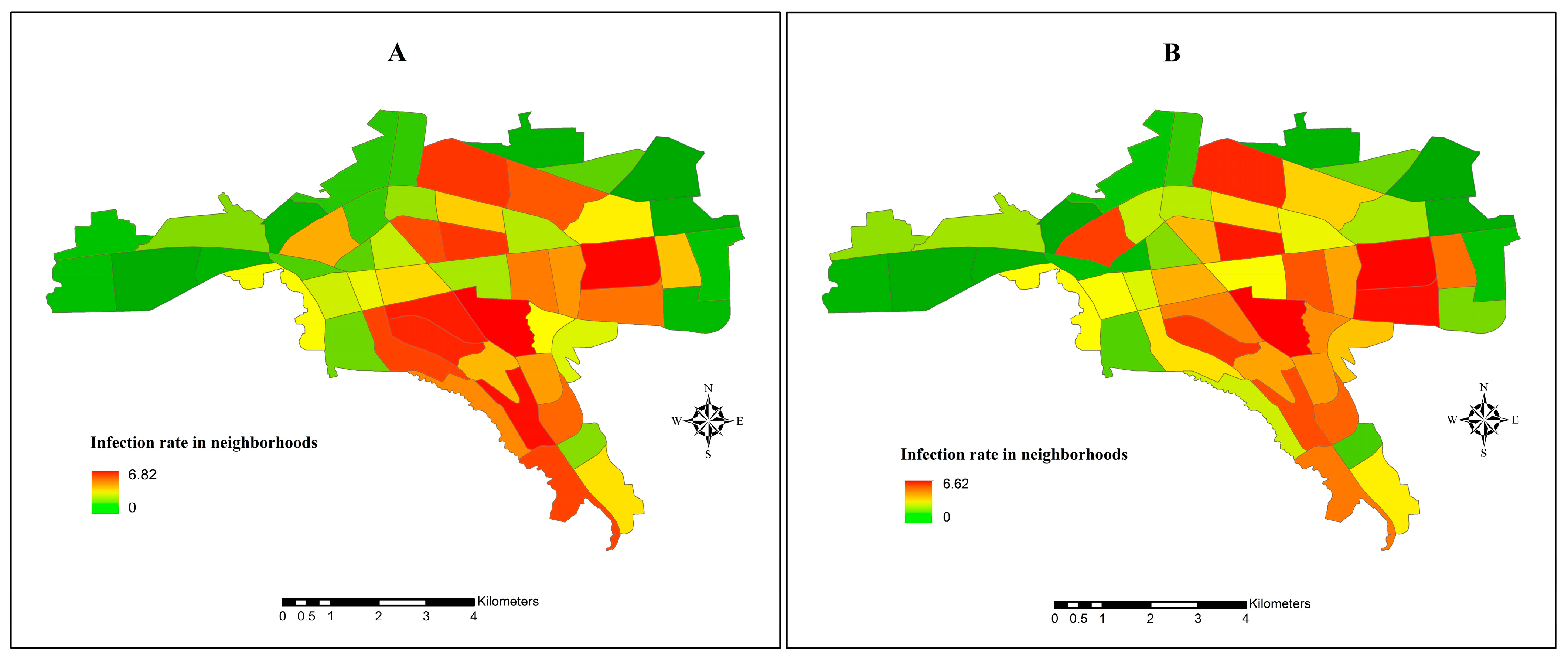
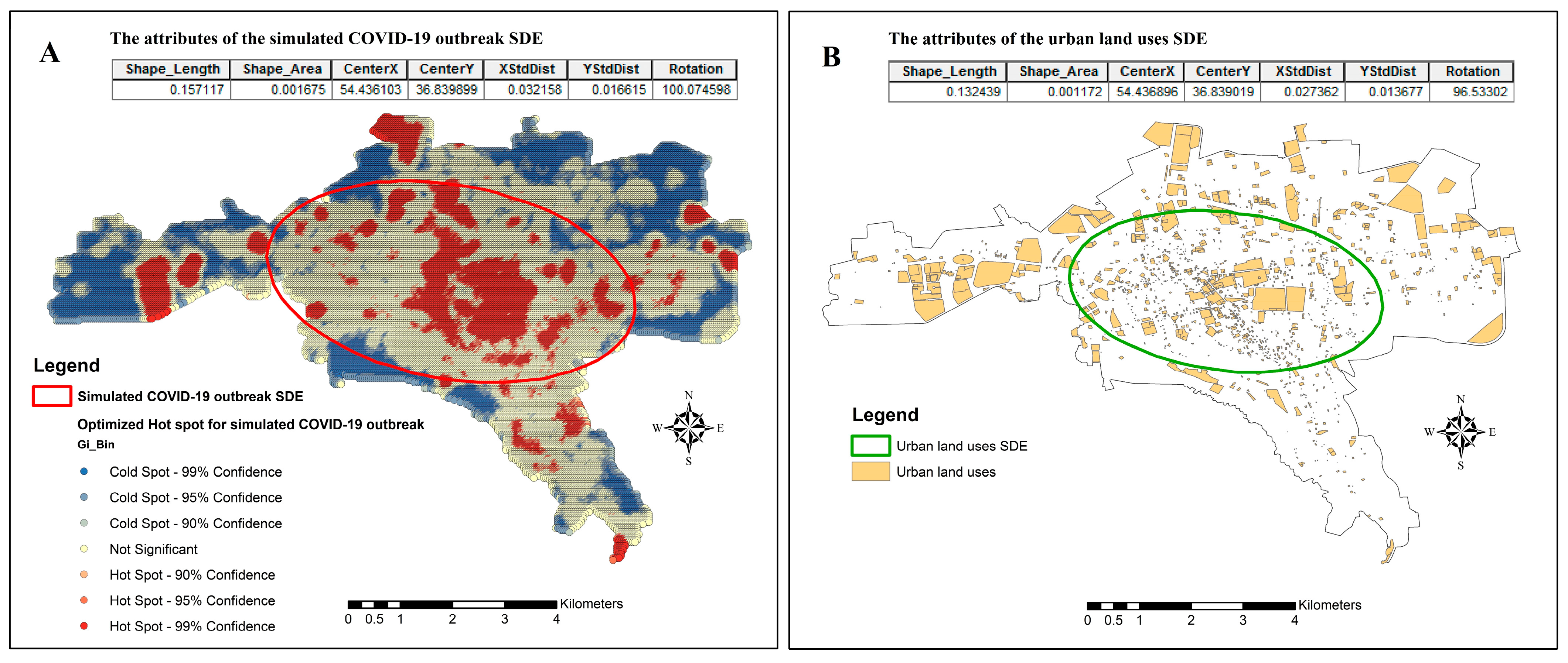
3.4. Spatial Spread of COVID-19

The susceptibility of the cellular agents was investigated at consecutive time points (on the 20th, 40th, 60th, 80th, and 100th days of the epidemic). According to Figure S1 (Supplementary Materials), the cells with higher susceptibilities correspond to the locations where COVID-19 has been most prevalent.

Figure 10 shows the spatial directional distribution of the COVID-19 outbreak (hot and cold spots after 100 days of the epidemic) and the urban land use across Gorgan. Figure 10A,B shows that the SDE parameters for the simulated COVID-19 outbreak and the urban land use, such as the center point, the semi-major axis, the semi-minor axis, and the directional angle, are relatively close; therefore, the spatial directional distribution of the simulated COVID-19 outbreak and the urban land use are very similar and mostly concentrated in the central areas of the city.

Furthermore, the vulnerability of each urban land use to the disease was explored. The proportion of infections that occurred in each type of land use to the total infections (as a percentage) is shown in Figure S2 (Supplementary Materials), indicating that the administrative land use account for the largest proportion of disease transmission, followed by recreational land use.

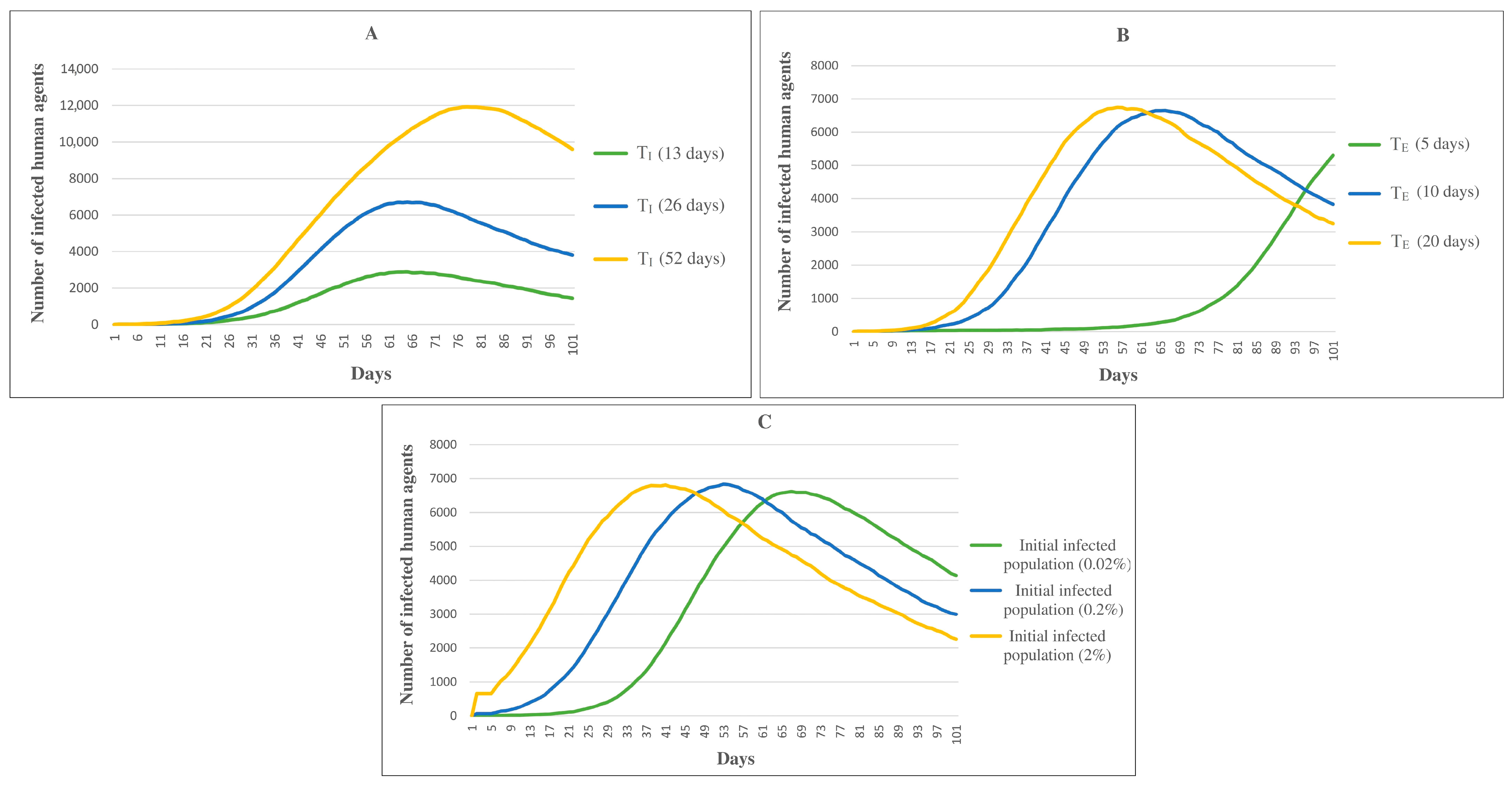
3.5. Temporal Trend of COVID-19

The good agreement of the values obtained for daily R₀ during the epidemic (between 1 and 3.09, with an average of 2.18) with its values in previous research [37,38,39] ascertained the reliability of the proposed model. As seen in Figure S3 (Supplementary Materials), with the onset of the epidemic, the weekly new cases and the weekly R₀ reach their peak during the fourth and fifth weeks of the epidemic (217 weekly new cases and weekly R₀ = 2.97) and then they decline. As the R₀ value decreases and gets closer to one, the disease reaches its endemic equilibrium phase.

4. Discussion

This study utilized an ABM to simulate the spatial spread of COVID-19 in Gorgan in northeast Iran with a heterogeneous spatial and demographic structure. The ABM considered the interactions between human agents and their environment by incorporating social activities based on different urban land use. The proposed model was integrated with the SASOARD epidemic model to better understand the transmission of the disease at the micro-level. The effect of various intervention scenarios on the epidemic was examined. In addition, the model’s behavior was assessed by varying key epidemic parameters, and evaluated in three modes of cases, deaths, and the spatial distribution of COVID-19. The results show that the disease was more concentrated in central areas with a high population density and dense urban land use. Furthermore, the proposed model could predict the distribution of disease cases and mortality based on different age groups with an accuracy of 72% and 71%, respectively, and the spatial distribution of disease cases at the neighborhood level with 86% accuracy. In addition, the results of the Chi-square test show that the predicted values in the mentioned modes are close enough to the corresponding observed values; therefore, these results increase the reliability of the proposed model.

The study investigated the effect of various intervention scenarios on the spread of the disease, including social distancing, complete and partial lockdowns, restriction of social gatherings, and vaccination. The social distancing scenario demonstrated a significant reduction in disease spread if implemented on the 10th day of the epidemic (Figure 6A). The results show that the peak of the epidemic was reduced by 98%. This is supported by the findings of Alagoz et al. [40], who showed that the timing of implementing social distancing could have a major impact on COVID-19 incidence. The partial lockdown scenario was found to have a lesser effect than the complete lockdown scenario, with a reduction of 13% and 86% at the epidemic’s peak when applied on the 10th day (Figure 6B,C). The restriction of social gatherings not only reduced the epidemic peak but also led to a delay in its emergence (Figure 6D). The vaccination scenario on the 10th day of the epidemic showed a 60% reduction of the epidemic’s peak and a 20-day delay in its occurrence (Figure 6E). The findings are consistent with Sah et al. [41], who showed that expediting population vaccination can reduce disease transmission. In general, early implementation of control scenarios can reduce COVID-19 transmission and even help control the transmission. The results indicate that social distancing and vaccination scenarios, when implemented in early stages of the outbreak, can have a greater impact to control the epidemic than other scenarios. Prioritizing these scenarios can help policymakers in their efforts to accelerate managing the epidemic; however, the effectiveness of these measures depends on the level of public compliance.

The spread of COVID-19 was found to be more concentrated in the central areas (Figure 10A), possibly due to the high population density and urban land use, which increase the likelihood of human contact and exposure to the virus. These findings are in line with the studies of Tabasi et al. [23], Xu et al. [42], and Razavi-Termeh et al. [43], who illustrated those areas with high population density, better economic status, higher socio-economic complexity, and a higher employment rate tend to have greater impacts on the spread of the disease. From a practical standpoint, urban managers can prevent the excessive spread of the disease in areas with high-density urban land use by designing urban land use in a decentralized manner in the urban environment. It may improve the resilience and sustainability of urban systems in the face of pandemics.

The results also show that different types of land use exhibit varying susceptibility to the disease. For instance, administrative land use that attracts a considerable portion of the population for daily activities was associated with a higher number of cases of COVID-19. On the other hand, despite a higher number of educational land use compared to commercial, recreational, and health land use, the prevalence of the disease was lower, possibly due to the lower severity of the disease in the age group of 3 to 24 years, who primarily use educational facilities. These findings highlight the importance of considering various factors in understanding the spread of COVID-19, such as the number of people utilizing different types of land use, the age group of people, and social gatherings. Health policymakers can utilize the findings to identify high-risk land use, restrict human mobility in these areas, and provide additional medical facilities to the residents of high-risk areas.

The findings indicate that the model has been able to identify the peak of the epidemic in the studied area. An analysis of the R₀ values shows that the peak of the epidemic occurs in the fourth and fifth weeks. In addition, when the disease reaches its endemic equilibrium state, the manageable daily new cases can be determined using the proposed model. Accordingly, this study can be useful in crafting policies that determine when the epidemic will peak and also identify the severity of the epidemic.

To our knowledge, previous ABM studies [44,45,46] mainly considered limited states for human agents; however, a human agent has more epidemic states, such as asymptomatic infected, symptomatic infected, on treatment, and aggravated infected. Moreover, previous studies generally have only focused on specific land use (e.g., colleges, supermarkets, offices, and religious land use) to model COVID-19 transmission [47,48,49,50,51,52,53]. For example, Bouchnita and Jebrane [16] implemented their ABM model with 250 human agents in a limited simulation environment (250 m × 250 m). They ignored heterogeneous social and geographic structures in their model. Cuevas [24] investigated the risk of COVID-19 transmission using a limited number of agents. This model has not been implemented in a real environment. The complex interactions and the heterogeneous demographic structures between agents were also ignored. Additionally, these studies have often focused on the temporal evolution of the pandemic and overlooked the spatial dynamics of the disease. For example, in the study by Mahdizadeh Gharakhanlou and Hooshangi [19], residential areas and the population of human agents were randomly distributed, precluding the analysis of spatial distribution of the disease. They only simulated human agents in four age groups: 0–5, 5–24, 24–64, and 64 years and older, while cases and deaths in other age groups are also common [5]. In addition, only limited types of urban land use, including schools, offices, and business areas, were included, while other land use types, such as health centers, universities, and recreational, cultural, and sports centers, can also be influential in the spread of the disease [23]. They assumed limited states of the epidemic situation (SEIRD) for a human agent. Furthermore, the effect of vaccination on the COVID-19 outbreak was not accounted for in their model.

This study has several limitations that should be acknowledged. The COVID-19 data used in the model were mostly extracted from previous studies, and the data accuracy was not fully investigated. Future work can consider uncertainties in the data and processes. The model assumed a closed environment, whereas humans can move out of the environment, which can be examined in future studies. This study assumed that all COVID-19 variants have similar virulence and transmissibility during the study period; however, this proposition is arguable, and it should be considered in future studies. The model also assumed complete immunity from re-infection for individuals who have received a vaccine or recovered from the disease, which is not realistic. Further research can examine the effect of different vaccine doses on the epidemic. Additionally, information about the control scenarios and people’s responsiveness to these measures was not available, as the primary focus of this study was on designing control scenarios and observing the changes in epidemic behaviors. In the future, more realistic assumptions and evaluations of the impact of these public health measures on the epidemic can be conducted by gathering such information. For example, the stringency index, which measures the degree of strictness of public health policies over time, can be incorporated into the model to improve the evaluation of public health measures.

5. Conclusions

This study has underscored the importance of ABMs in modeling the COVID-19 spread at the individual level under various scenarios in an urban environment. In this study, four principles of spatial ABMs were presented [54], which include designing the behavior of agents and the environment, considering heterogeneous spatial and demographic structures in the model, model verification and validation, and extracting spatial patterns of the disease by the model. To implement these principles, the behavior of human agents was defined through the SASOARD model and the time pattern of human activities based on urban land use. The results demonstrate that COVID-19 is more prevalent in the central areas of Gorgan, which have high population density and dense urban land use. This finding provides an interesting perspective for urban managers in the post-pandemic period to design urban land use in a decentralized manner in the urban environment, which slows down the spread of COVID-19 and thereby improves the preparedness and resilience of communities in the face of future pandemics. The study has also showed that the social distancing and vaccination scenarios applied in the early stages of the epidemic could have the most significant impacts in controlling the spread of the disease. This study can enlighten health managers and urban planners to understand the spatial spread of the disease, design control scenarios for allocating resources to high-risk areas and vulnerable populations more effectively, and construct a sustainable and resilient urban system to deal with future pandemic events.

References

1. Mathieu, E.; Ritchie, H.; Rodés-Guirao, L.; Appel, C.; Giattino, C.; Hasell, J.; Macdonald, B.; Dattani, S.; Beltekian, D.; Ortiz-Ospina, E.; et al. Coronavirus Pandemic (COVID-19). Our World in Data 2020. Available online: https://ourworldindata.org/coronavirus (accessed on 7 January 2023).
2. World Health Organization. Novel Coronavirus (2019-nCoV) Situation Reports; World Health Organization: Geneva, Switzerland, 2020. Available online: https://www.who.int/emergencies/diseases/novel-coronavirus-2019/situation-reports (accessed on 4 April 2020).
3. Babaie, E.; Alesheikh, A.A.; Tabasi, M. Spatial prediction of human brucellosis (HB) using a GIS-based adaptive neuro-fuzzy inference system (ANFIS). Acta Trop. 2021, 220, 105951. [Google Scholar] [CrossRef] [PubMed]
4. Razavi-Termeh, S.V.; Sadeghi-Niaraki, A.; Choi, S.M. Spatio-temporal modelling of asthma-prone areas using a machine learning optimized with metaheuristic algorithms. Geocarto Int. 2022, 37, 9917–9942. [Google Scholar] [CrossRef]
5. Tabasi, M.; Alesheikh, A.A.; Babaie, E.; Hatamiafkoueieh, J. Spatiotemporal Surveillance of COVID-19 Based on Epidemiological Features: Evidence from Northeast Iran. Sustainability 2022, 14, 12189. [Google Scholar] [CrossRef]
6. Masrur, A.; Yu, M.; Luo, W.; Dewan, A. Space-time patterns, change, and propagation of COVID-19 risk relative to the intervention scenarios in Bangladesh. Int. J. Environ. Res. Public Health 2020, 17, 5911. [Google Scholar] [CrossRef]
7. Anastassopoulou, C.; Russo, L.; Tsakris, A.; Siettos, C. Data-based analysis, modelling and forecasting of the COVID-19 outbreak. PLoS ONE 2020, 15, 0230405. [Google Scholar] [CrossRef]
8. Barlow, N.S.; Weinstein, S.J. Accurate closed-form solution of the SIR epidemic model. Phys. D Nonlinear Phenom. 2020, 408, 132540. [Google Scholar] [CrossRef]
9. Weissman, G.E.; Crane-Droesch, A.; Chivers, C.; Luong, T.; Hanish, A.; Levy, M.Z.; Lubken, J.; Becker, M.; Draugelis, M.E.; Anesi, G.L.; et al. Locally informed simulation to predict hospital capacity needs during the COVID-19 pandemic. Ann. Intern. Med. 2020, 173, 21–28. [Google Scholar] [CrossRef]
10. Kuniya, T. Prediction of the epidemic peak of coronavirus disease in Japan, 2020. J. Clin. Med. 2020, 9, 789. [Google Scholar] [CrossRef]
11. Tuite, A.R.; Fisman, D.N.; Greer, A.L. Mathematical modelling of COVID-19 transmission and mitigation strategies in the population of Ontario, Canada. Can. Med. Assoc. J. 2020, 192, E497–E505. [Google Scholar] [CrossRef]
12. Kelly, R.A.; Jakeman, A.J.; Barreteau, O.; Borsuk, M.E.; ElSawah, S.; Hamilton, S.H.; Henriksen, H.J.; Kuikka, S.; Maier, H.R.; Rizzoli, A.E.; et al. Selecting among five common modelling approaches for integrated environmental assessment and management. Environ. Model. Softw. 2013, 47, 159–181. [Google Scholar] [CrossRef]
13. Germann, T.C.; Kadau, K.; Longini, I.M., Jr.; Macken, C.A. Mitigation strategies for pandemic influenza in the United States. Proc. Natl. Acad. Sci. USA 2006, 103, 5935–5940. [Google Scholar] [CrossRef]
14. Longini, I.M., Jr.; Nizam, A.; Xu, S.; Ungchusak, K.; Hanshaoworakul, W.; Cummings, D.A.; Halloran, M.E. Containing pandemic influenza at the source. Science 2005, 309, 1083–1087. [Google Scholar] [CrossRef]
15. Banisch, S. Markov Chain Aggregation for Agent-Based Models; Springer: Berlin/Heidelberg, Germany, 2015. [Google Scholar]
16. Bouchnita, A.; Jebrane, A. A hybrid multi-scale model of COVID-19 transmission dynamics to assess the potential of non-pharmaceutical interventions. Chaos Solitons Fractals 2020, 138, 109941. [Google Scholar] [CrossRef]
17. Zhou, S.; Zhou, S.; Zheng, Z.; Lu, J. Optimizing spatial allocation of COVID-19 vaccine by agent—Based spatiotemporal simulations. GeoHealth 2021, 5, e2021GH000427. [Google Scholar] [CrossRef] [PubMed]
18. Tabasi, M.; Alesheikh, A.A.; Sofizadeh, A.; Saeidian, B.; Pradhan, B.; AlAmri, A. A spatio-temporal agent-based approach for modeling the spread of zoonotic cutaneous leishmaniasis in northeast Iran. Parasites Vectors 2020, 13, 572. [Google Scholar] [CrossRef]
19. Gharakhanlou, N.M.; Hooshangi, N. Spatio-temporal simulation of the novel coronavirus (COVID-19) outbreak using the agent-based modeling approach (case study: Urmia, Iran). Inform. Med. Unlocked 2020, 20, 100403. [Google Scholar] [CrossRef] [PubMed]
20. Olszewski, R.; Pałka, P.; Wendland, A. Agent-based modeling as a tool for predicting the spatial-temporal diffusion of the COVID-19 pandemic. In Proceedings of the 2021 IEEE International Conference on Industrial Engineering and Engineering Management (IEEM), Singapore, 11–15 December 2021. [Google Scholar]
21. COVID-19 Cases Data in Golestan Province, 2020–2021: Iranian Ministry of Health, Center for Disease Control and Prevention (CDC) of Golestan Province; Unpublished Data. 2021. Available online: https://goums.ac.ir/index.php?slc_lang=en&sid=200 (accessed on 28 February 2021).
22. Census Data and Land Use Data in Golestan Province, 2020–2021: Statistical Center of Iran, Deputy of Statistics and Information of Golestan Province. 2021. Available online: https://amar.golestanmporg.ir/ (accessed on 10 February 2022).
23. Tabasi, M.; Alesheikh, A.A.; Kalantari, M.; Babaie, E.; Mollalo, A. Spatial Modeling of COVID-19 Prevalence Using Adaptive Neuro-Fuzzy Inference System. ISPRS Int. J. Geo-Inf. 2022, 11, 499. [Google Scholar] [CrossRef]
24. Cuevas, E. An agent-based model to evaluate the COVID-19 transmission risks in facilities. Comput. Biol. Med. 2020, 121, 103827. [Google Scholar] [CrossRef]
25. Dascalu, M.; Malita, M.; Barbilian, A.; Franti, E.; Stefan, G.M. Enhanced cellular automata with autonomous agents for covid-19 pandemic modeling. Rom. J. Inf. Sci. Technol. 2020, 23, S15–S27. [Google Scholar]
26. Kai, D.; Goldstein, G.; Morgunov, A.; Nangalia, V.; Rotkirch, A. Universal masking is urgent in the COVID-19 pandemic: SEIR and agent based models, empirical validation, policy recommendations. arXiv 2020, arXiv:2004.13553. [Google Scholar]
27. Kontokosta, C.E.; Hong, B.; Bonczak, B.J. Measuring sensitivity to social distancing behavior during the COVID-19 pandemic. Sci. Rep. 2022, 12, 16350. [Google Scholar] [CrossRef] [PubMed]
28. Setti, L.; Passarini, F.; De Gennaro, G.; Barbieri, P.; Perrone, M.G.; Borelli, M.; Palmisani, J.; Di Gilio, A.; Piscitelli, P.; Miani, A. Airborne transmission route of COVID-19: Why 2 meters/6 feet of inter-personal distance could not be enough. Int. J. Environ. Res. Public Health 2020, 17, 2932. [Google Scholar] [CrossRef] [PubMed]
29. Bi, Q.; Wu, Y.; Mei, S.; Ye, C.; Zou, X.; Zhang, Z.; Liu, X.; Wei, L.; Truelove, S.A.; Zhang, T.; et al. Epidemiology and transmission of COVID-19 in 391 cases and 1286 of their close contacts in Shenzhen, China: A retrospective cohort study. Lancet Infect. Dis. 2020, 20, 911–919. [Google Scholar] [CrossRef]
30. Moore_Neighborhood. Available online: https://en.wikipedia.org/wiki/Moore_neighborhood (accessed on 20 February 2023).
31. Kerr, C.C.; Stuart, R.M.; Mistry, D.; Abeysuriya, R.G.; Rosenfeld, K.; Hart, G.R.; Núñez, R.C.; Cohen, J.A.; Selvaraj, P.; Hagedorn, B.; et al. Covasim: An agent-based model of COVID-19 dynamics and interventions. PLoS Comput. Biol. 2021, 17, e1009149. [Google Scholar] [CrossRef]
32. World Health Organization. Getting the COVID-19 Vaccine. 2021. Available online: https://www.who.int/news-room/feature-stories/detail/getting-the-covid-19-vaccine (accessed on 31 March 2021).
33. Xiang, X.; Kennedy, R.; Madey, G.; Cabaniss, S. Verification and validation of agent-based scientific simulation models. In Proceedings of the Agent-Directed Simulation Conference, San Diego, CA, USA, 14–17 April 2005; Volume 47, p. 55. [Google Scholar]
34. Getis, A.; Ord, J.K. The analysis of spatial association by use of distance statistics. In Perspectives on Spatial Data Analysis; Springer: Berlin/Heidelberg, Germany, 2010; pp. 127–145. [Google Scholar]
35. Mitchell, A. The ESRI Guide to GIS Analysis; Esri Press: Redlands, CA, USA, 2005; Volume 2, Available online: https://www.esri.com/en-us/esri-press/browse/the-esri-guide-to-gis-analysis-volume-2-spatial-measurements-and-statistics-second-edition (accessed on 10 February 2022).
36. Manore, C.A.; Hickmann, K.S.; Hyman, J.M.; Foppa, I.M.; Davis, J.K.; Wesson, D.M.; Mores, C.N. A network-patch methodology for adapting agent-based models for directly transmitted disease to mosquito-borne disease. J. Biol. Dyn. 2015, 9, 52–72. [Google Scholar] [CrossRef] [PubMed]
37. Zhao, S.; Lin, Q.; Ran, J.; Musa, S.S.; Yang, G.; Wang, W.; Lou, Y.; Gao, D.; Yang, L.; He, D.; et al. Preliminary estimation of the basic reproduction number of novel coronavirus (2019-nCoV) in China, from 2019 to 2020: A data-driven analysis in the early phase of the outbreak. Int. J. Infect. Dis. 2020, 92, 214–217. [Google Scholar] [CrossRef]
38. Zhang, S.; Diao, M.; Yu, W.; Pei, L.; Lin, Z.; Chen, D. Estimation of the reproductive number of novel coronavirus (COVID-19) and the probable outbreak size on the Diamond Princess cruise ship: A data-driven analysis. Int. J. Infect. Dis. 2020, 93, 201–204. [Google Scholar] [CrossRef]
39. Li, Q.; Guan, X.; Wu, P.; Wang, X.; Zhou, L.; Tong, Y.; Ren, R.; Leung, K.S.; Lau, E.H.; Wong, J.Y.; et al. Early transmission dynamics in Wuhan, China, of novel coronavirus–infected pneumonia. N. Engl. J. Med. 2020, 382, 1199–1207. [Google Scholar] [CrossRef]
40. Alagoz, O.; Sethi, A.K.; Patterson, B.W.; Churpek, M.; Safdar, N. Effect of timing of and adherence to social distancing measures on COVID-19 burden in the United States: A simulation modeling approach. Ann. Intern. Med. 2021, 174, 50–57. [Google Scholar] [CrossRef]
41. Sah, P.; Vilches, T.N.; Moghadas, S.M.; Fitzpatrick, M.C.; Singer, B.H.; Hotez, J.; Galvani, A. Accelerated vaccine rollout is imperative to mitigate highly transmissible COVID-19 variants. eClinicalMedicine 2021, 35, 100865. [Google Scholar] [CrossRef]
42. Xu, J.; Deng, Y.; Yang, J.; Huang, W.; Yan, Y.; Xie, Y.; Li, Y.; Jing, W. Effect of Population Migration and Socioeconomic Factors on the COVID-19 Epidemic at County Level in Guangdong, China. Front. Environ. Sci. 2022, 10, 841996. [Google Scholar] [CrossRef]
43. Razavi-Termeh, S.V.; Sadeghi-Niaraki, A.; Farhangi, F.; Choi, S.M. COVID-19 risk mapping with considering socio-economic criteria using machine learning algorithms. Int. J. Environ. Res. Public Health 2021, 18, 9657. [Google Scholar] [CrossRef] [PubMed]
44. Chung, N.N.; Chew, L.Y. Modelling Singapore COVID-19 pandemic with a SEIR multiplex network model. Sci. Rep. 2021, 11, 10122. [Google Scholar] [CrossRef] [PubMed]
45. Zhou, Y.; Li, L.; Ghasemi, Y.; Kallagudde, R.; Goyal, K.; Thakur, D. An agent-based model for simulating COVID-19 transmissions on university campus and its implications on mitigation interventions: A case study. Inf. Discov. Deliv. 2021, 49, 216–224. [Google Scholar] [CrossRef]
46. Alsaeed, N.I.; Alqaissi, E.Y.; Siddiqui, M.A. An Agent-based Simulation of the SIRD model of COVID-19 Spread. Int. J. Biol. Biomed. Eng. 2020, 14, 210–217. [Google Scholar]
47. Ying, F.; O’Clery, N. Modelling COVID-19 transmission in supermarkets using an agent-based model. PLoS ONE 2021, 16, e0249821. [Google Scholar] [CrossRef]
48. Bahl, R.; Eikmeier, N.; Fraser, A.; Junge, M.; Keesing, F.; Nakahata, K.; Reeves, L. Modeling COVID-19 spread in small colleges. PLoS ONE 2021, 16, e0255654. [Google Scholar] [CrossRef]
49. Scott, N.; Palmer, A.; Delport, D.; Abeysuriya, R.; Stuart, R.M.; Kerr, C.C.; Mistry, D.; Klein, D.J.; Sacks-Davis, R.; Heath, K.; et al. Modelling the impact of relaxing COVID-19 control measures during a period of low viral transmission. Med. J. Aust. 2021, 214, 79–83. [Google Scholar] [CrossRef]
50. Gressman, T.; Peck, J.R. Simulating COVID-19 in a university environment. Math. Biosci. 2020, 328, 108436. [Google Scholar] [CrossRef]
51. Jarvis, K.F.; Kelley, J.B. Temporal dynamics of viral load and false negative rate influence the levels of testing necessary to combat COVID-19 spread. Sci. Rep. 2021, 11, 9221. [Google Scholar] [CrossRef]
52. Alvarez Castro, D.; Ford, A. 3D agent-based model of pedestrian movements for simulating COVID-19 transmission in university students. ISPRS Int. J. Geo-Inf. 2021, 10, 509. [Google Scholar] [CrossRef]
53. Al-Shaery, A.M.; Hejase, B.; Tridane, A.; Farooqi, N.S.; Jassmi, H.A. Agent-based modeling of the Hajj Rituals with the possible spread of COVID-19. Sustainability 2021, 13, 6923. [Google Scholar] [CrossRef]
54. Filatova, T.; Verburg, P.H.; Parker, D.C.; Stannard, C.A. Spatial agent-based models for socio-ecological systems: Challenges and prospects. Environ. Model. Softw. 2013, 45, 1–7. [Google Scholar] [CrossRef]
Figure 1. The geographical location of Iran (A), Golestan province (B), and Gorgan and its 52 neighborhoods (C).
Sustainability 15 13827 g001
Figure 2. Population of blocks (A) and types of urban land use (B) in Gorgan.
Sustainability 15 13827 g002
Figure 3. The ABM components (agent types, agent characteristics, and behaviors of agents in the environment) using the UML diagram.
Sustainability 15 13827 g003
Figure 4. Overview of the scheduling process sequence at each time step using the UML sequence diagram.
Sustainability 15 13827 g004
Figure 5. Daily social activities for human agents according to age groups.
Sustainability 15 13827 g005
Figure 6. The trend of the COVID-19 outbreak by applying different scenarios: social distancing (A), complete lockdown (B), partial lockdown (C), restriction in social gatherings (D), and vaccination (E).
Sustainability 15 13827 g006
Figure 7. The epidemic of COVID-19 regarding varying key parameters of interest: the TI (A), the TE (B), and the initial infected population (C).
Sustainability 15 13827 g007
Figure 8. Comparison of the predicted infection rate with the observed infection rate based on age groups (A). Comparison of the predicted mortality rate with the observed death rate for different age groups (B).
Sustainability 15 13827 g008
Figure 9. Comparing the observed infection rate (A) with the predicted infection rate (B) at the neighborhood level in Gorgan.
Sustainability 15 13827 g009
Figure 10. The standard deviation ellipse of the simulated COVID-19 outbreak (A) and the urban land use (B).
Sustainability 15 13827 g010