Effective Load Frequency Control of Power System with Two-Degree Freedom Tilt-Integral-Derivative Based on Whale Optimization Algorithm

Abstract

Nowadays, the operation and control of power systems are a big challenge. An essential part of the power system (PS) control is load frequency control (LFC). Different secondary controllers are implemented for the frequency control problem. Hence, cascaded two-degree freedom and a tilt-integral-derivative controller having a filter (2DOFTIDF) are intended in this paper and implemented for load frequency control. In order to determine the efficiency of the 2DOFTIDF controller, a well-known non-reheat thermal system with/without a governor dead band is considered. A new whale optimization algorithm (WOA) is used to enhance the suggested controller parameters. The predominance of the presented method is exhibited by comparing the consequences with different heuristic techniques tuned to controllers published recently. Further, the simulation results for two test cases indicate that system enactments are enhanced by introducing the suggested controller and are also best suited in the presence of system nonlinearity. Finally, random load fluctuation along with noise and changing the system parameters are also used to determine the reliability of the suggested controller. Compared to the WOA-tuned TIDF controller, the settling time of ΔF₁, ΔF_2, and ΔP_Tie is improved by 45.45%, 56.77%, and 20.26%, respectively, with the WOA-tuned 2DOFTIDF controller and by 40%, 48.27%, and 20%, respectively, with the DE-tuned TIDF controller. Experimental validation using the hardware-in-the-loop real-time simulation based on OPAL-RT has been carried out to confirm the viability of the proposed approach.

1. Introduction

Frequency is critical in operating a power system (PS) network smoothly and satisfactorily. The deviation in supply frequency will cause an increase in iron losses, magnetizing current drawn by the induction motor from the source, and the variation in the synchronous speed of the synchronous machine [1,2,3,4]. In order to overcome the above difficulties, the generated power should equal or satisfy the power demanded by the loads. Therefore, the supply frequency should be preserved at a rated value. However, unfortunately, in an interconnected power system, the load is continuously varying; frequency is also varying. Therefore, the frequency control loop must continually change the generator’s active power output to satisfy the load requirement and maintain frequency at a nominal value. Load frequency control (LFC) reduces frequency deviations and steady-state errors [5]. LFC plays a vital role in PS due to its increased size and complexity [6].

Many researchers worldwide investigated different control techniques and implemented optimization methods to reduce steady-state errors that limit the frequency. Saikia et al. proposed bacteria foraging optimization algorithm (BFOA)-optimized proportional-integral-derivative (PID), integral double derivative (IDD), proportional-integral (PI), integral (I), and integral-derivative (ID) controllers to solve the LFC problem in multi-area PS [7]. The authors in [8] proposed an imperialist competitive algorithm (ICA), which is utilized to tune PID controllers for a multi-area multi-source system. Panda et al. [9] introduced hybrid algorithms combining bacteria foraging optimization and particle swarm optimization (hBFOA-PSO), which are used to tune the PI controller for AGC. Authors in [10] presented a flower pollination algorithm (FPA)-tuned PID controller design to reduce PS frequency deviations with governor dead band. Abdelaziz and Ali [11] proposed an artificial cuckoo search technique for LFC design. Furthermore, Abo-Elyousr and Abdelaziz [12] suggested a hybrid PSO-WOA technique for LFC design. A literature survey also reveals that fuzzy logic controllers [13], Artificial Neural Networks (ANN) [14], sliding mode controllers [15], and type-2 fuzzy controllers [16] were also used to solve LFC problems. The above survey shows that there is always a span for designing a new controller for the abovementioned problem. Hiroi et al. [17] developed a two degrees of freedom PID (2DOFPID) controller that improves set point detection and control in the presence of disturbance inputs in a plant process. Sahu et al. [18] proposed a differential evolution (DE)-optimized 2DOFPID controller for the two-area power system. To improve frequency stability during system transient intervals, M.M Elsaied et al. [19] suggested a new Jellyfish Search Optimizer-based TID controller. The Fractional Order Integral-Tilt Derivative (FOI-TD) controller presented by Amil Daraz et al. [20], optimized by the Improved-Fitness Dependent Optimizer (I-FDO) algorithm, performs better under realistic situations to reduce the frequency inaccuracy. Debbarma et al. [21] introduced a 2DOF fractional PID controller for an unequal three-area reheat thermal system by considering the generation rate constraint (GRC) as nonlinearity. Lurie et al. [22] invented a tilt integral derivative controller (TID) to attain a good feedback compensator for the plant. In a PID controller, a tilting component with a transfer function of “s” to the power replaces the proportional component to create a TID controller, which gives simple tuning, improved disturbance rejection, and is less sensitive to parameter variation of a plant on closed-loop response. The term ‘n’ in the tilted compensator is the non-zero real number component. The authors proposed a TID controller having a filter (TIDF) in Ref. [23] to resolve frequency problems in nonlinear multi-area power systems. The filter is considered with the derivative controller to reduce unnecessary chattering problems. The TID controller is also successfully applied in different fields such as in magnetic levitation systems [24] and excitation control of synchronous generators [25]. This motivated the author to consider TIDF as a secondary controller. The principle of 2DOF is applied to PID [18] and fractional PID [21] controllers, and better results are achieved than in single-degree PID and fractional PID controllers. Surprisingly, this concept is not applied to the TIDF controller. However, based on the author’s knowledge, these two control techniques were not previously studied for AGC or any engineering problem. For the first time, the concept of 2DOF is applied to the TIDF controller structure to accomplish a new controller, the 2DOFTIDF controller. Hence, for the first time, a 2DOFTIDF controller is employed in this article for LFC problems in interconnected power systems. Excitation control and LFC are mutually coupled with each other. Until now, researchers studied LFC separately without considering the effect of excitation control. A change in load does not affect excitation control, whereas a change in excitation affects system dynamics. Therefore, this paper applies a step change in voltage to study the impact of frequency, tie-line power, and power dispatch on a different area of the considered system.

The literature study on LFC discloses that the controller parameters should be tuned using robust optimization techniques to obtain the optimal solution and improve performance. Recent meta-heuristic methods such as the bat algorithm (BA) [26], DE [18], grey wolf optimization (GWO) algorithm [27], cuckoo search (CS) [28], firefly algorithm (FA) [29], and MFO [30], etc., are successfully applied to tune different controllers for the AGC system. Researchers develop different algorithms to solve various engineering problems. Mirjalili recently developed the whale optimization algorithm (WOA) algorithm [31], which was successfully used in a hybrid PS. WOA is also applied for the 2DOF state feedback controller to minimize frequency errors [32] and maximum power point tracking (MPPT) for solar PV [33]. It is understood that WOA provides enhanced performance than other evolutionary algorithms. WOA provides a globally optimal solution by excluding local optima because of its exploration and exploitation phases. Therefore, a meta-heuristic technique known as the WOA is employed that optimizes the proposed 2DOFTIDF controller’s parameter.

In view of the findings, this paper investigates the frequency stability analysis of PS considering the two-degree freedom tilt-integral-derivative structured controller. In this present work, the following objectives are accomplished.

• Frequency stability analysis is performed for interconnected power systems on sudden application of disturbance.
• The 2DOFTID controller is designed to achieve better stability over PID and TIDF controllers for the same system with the same disturbances. Effectiveness of the proposed 2DOFTIDF controller is verified by adding nonlinearity to the system.
• WOA is employed to find the optimum parameters.
• The WOA algorithm’s effectiveness is determined by contrasting the system outcomes with other optimization techniques.
• The proposed 2DOFTIDF controller offers better performance compared to other classical controllers in multi-area multi-source power systems.
• A practical power system model is established considering the coupling effect of excitation control and LFC loop.
• The impact of parameter variation on the controller’s resilience is presented.
• MATLAB/Simulink results are contrasted with hardware-in-the-loop (HiL) real-time simulation data for experimental validation of the proposed method.

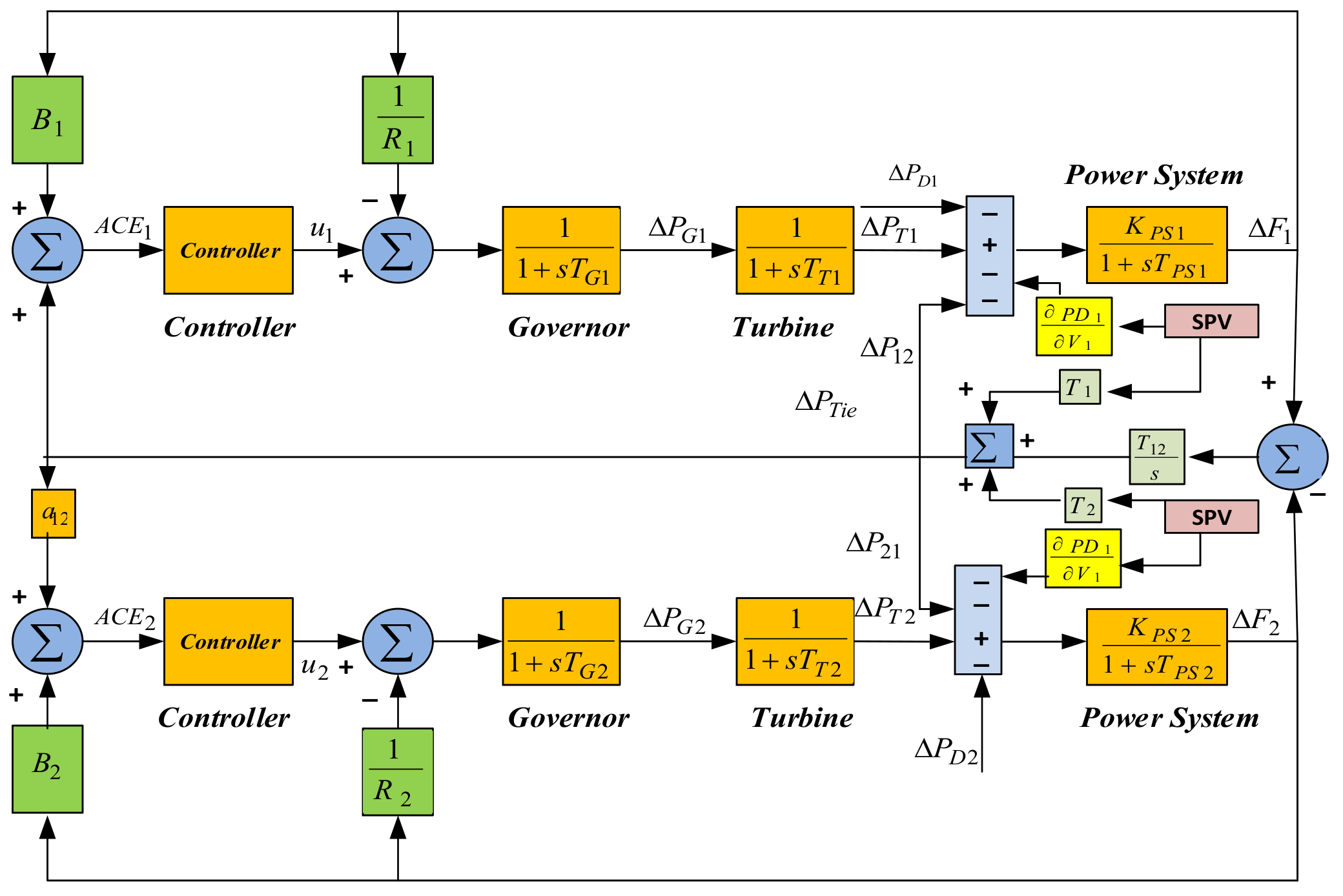
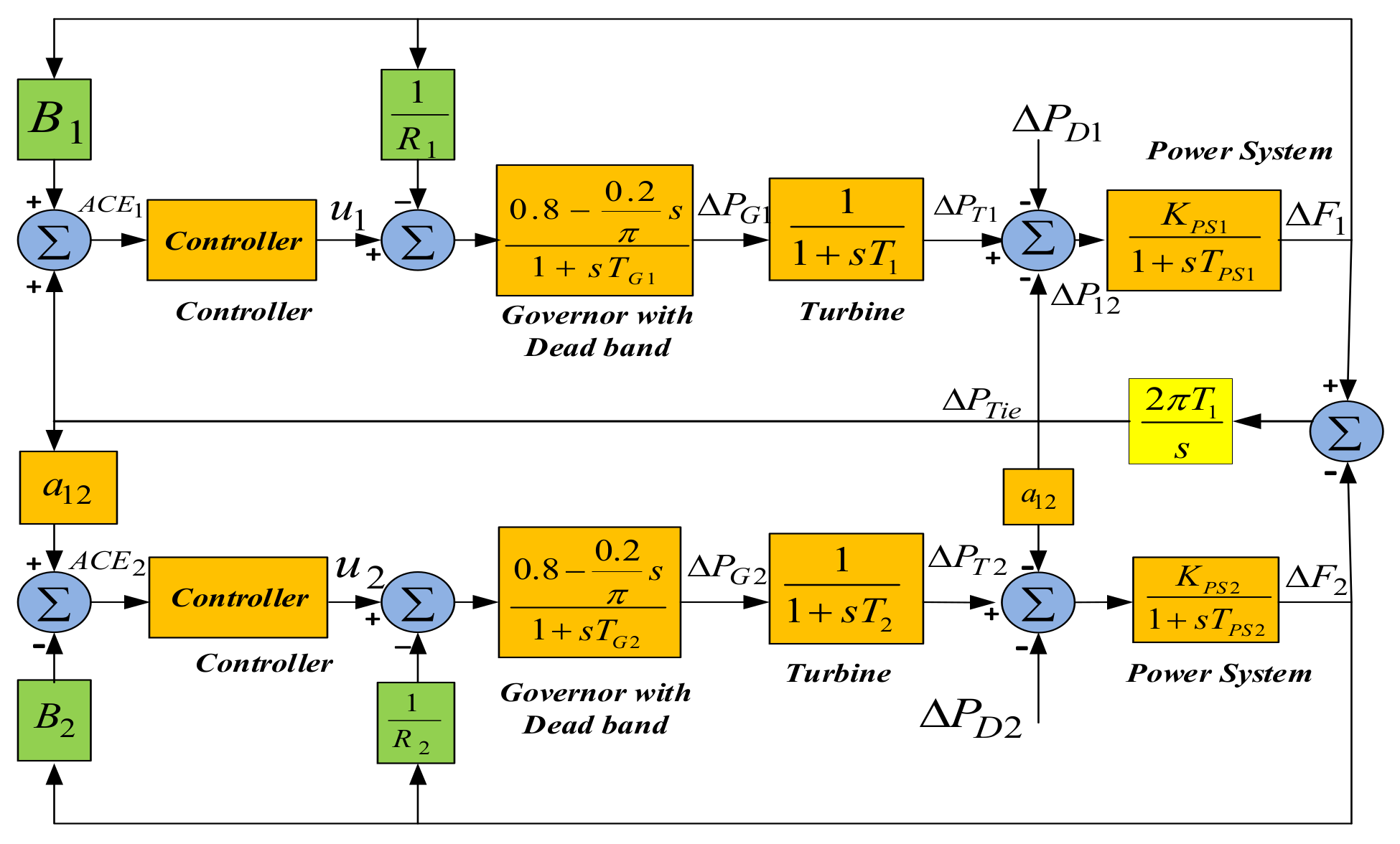
The rest of this article is structured as follows. The system modeling is investigated in Section 2. The overview of the control structure is deliberated in Section 3. Section 4 elucidates about the whale optimization algorithm. The problem-solving scenarios are presented in Section 5, and Section 6 concludes the paper.

2. System Modeling

The simulation studies were conducted on two areas with non-reheat thermal power stations. Figure 1 portrays the transfer function model of the system [23]. The rating of each area is 2000 MW, and the nominal load of each area is 1000 MW. In Figure 1, governor time constants are T_g1 and T_g2 in a sec; turbine time constants are T_t1 and T_t2 in a sec; PS gains are K_ps1 and K_ps2; PS time constants are T_ps1 and T_ps2 in a sec; frequency bias constants are B₁ and B₂; speed regulation constants are R₁ and R₂ of areas 1 and 2, respectively; T₁₂ shows the synchronizing time constant; ΔP_L is load disturbance; ΔF₁ and ΔF₂ are frequency deviations at areas 1 and 2, respectively; and ΔPtie is the deviation occurring in tie-line power. The nominal values of the system are presented in Appendix A.1.

Practically, in a power system, LFC and excitation control are cross-coupled to each other. An exact power system model is developed considering the above effect. The tie-line power is formulated as follows:

$$P_{tie}=\frac{\left|V_1\right|\left|V_2\right|}{X_{12}}\sin \left({\delta }_1-{\delta }_2\right)$$

(1)

where the voltage magnitudes of both areas are |V₁| and |V₂|, tie-line reactance is X₁₂, and power angles of both areas are δ₁, and δ₂, respectively. In several published research works, P_tie is only derived from δ₁ and δ₂ when a constant voltage magnitude is assumed [5].

To create a precise model for $\partial$Ptie, ∆|V₁| and ∆|V₂| should be considered as follows:

$$\Delta P_{tie}=\frac{\partial P_{tie}}{{\partial V}_1}\Delta V_1+\frac{\partial P_{tie}}{{\partial V}_2}\Delta V_2+\frac{\partial P_{tie}}{\partial \left({\delta }_1-{\delta }_2\right)}\Delta \left({\delta }_1-{\delta }_2\right)$$

(2)

Equation (2) can be written in another way as expressed by

$$\Delta P_{tie}=T_1\Delta V_1+T_2\Delta V_2+T_{12}\Delta \left({\delta }_1-{\delta }_2\right)$$

(3)

where the coefficients T₁ and T₂ are expressed as follows:

$$T_{{}_1}=\frac{V_2^0}{X_{12}}\sin \left({\delta }_1^0-{\delta }_2^0\right)$$

(4)

$$T_{{}_1}=\frac{V_1^0}{X_{12}}\sin \left({\delta }_1^0-{\delta }_2^0\right)$$

(5)

Exciter voltage perturbations of both areas are added to the tie-line power change with the system model. In addition, loads are added by an amount of $\frac{\partial {PD}_1}{\partial V_1}\Delta V_1$ and $\frac{\partial {PD}_2}{\partial V_2}\Delta V_2$ to both control areas.

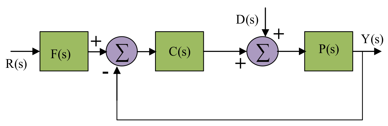
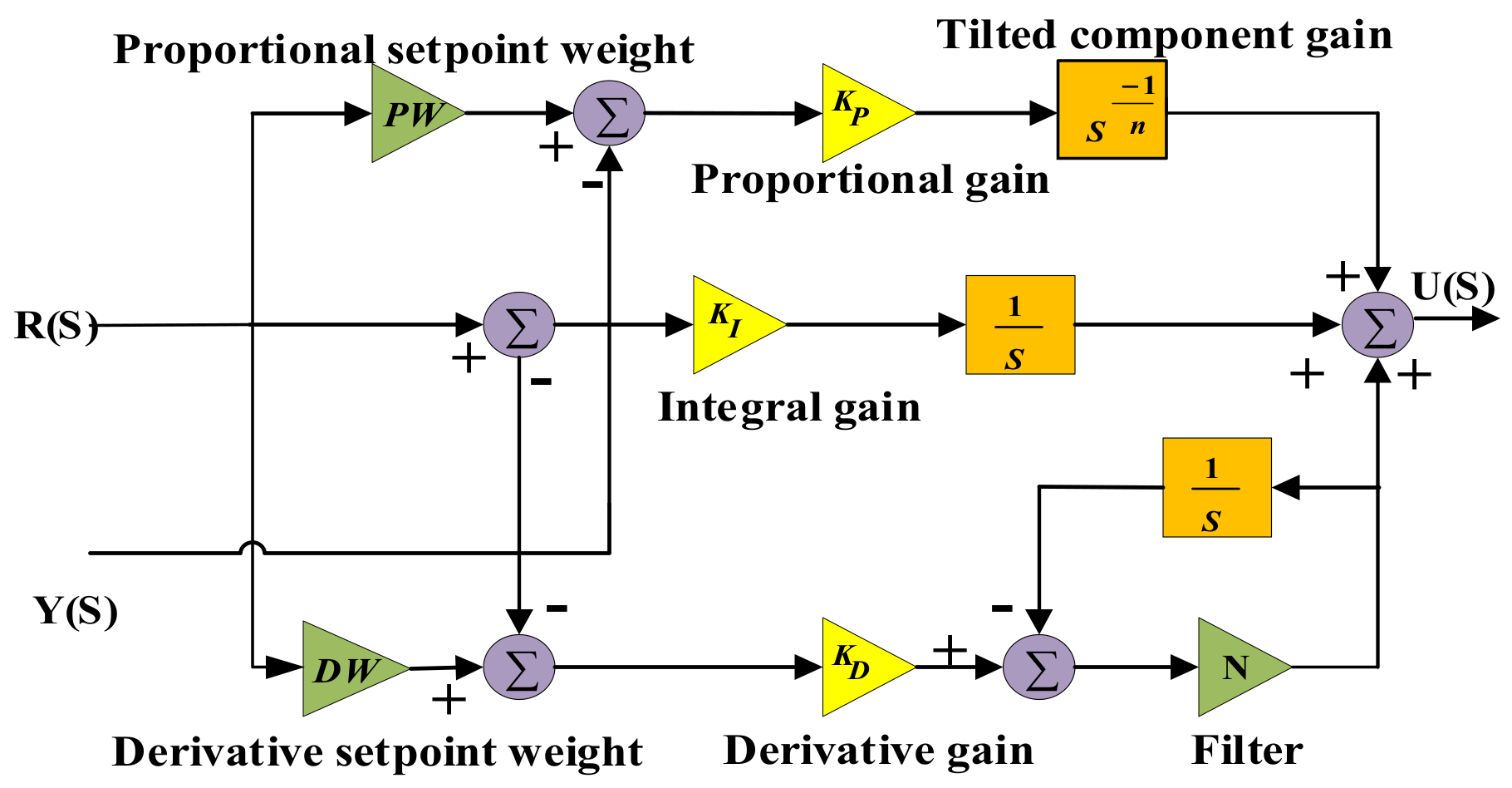
3. Control Structure

The TID controller is one of the fascinating fractional order controllers first introduced in [22]. Its implementation is straightforward in feedback systems as it uses a traditional PID controller. For modeling this controller, the tilt controller with a transfer function, $S^{\frac{-1}{n}}$ is multiplied by the proportional component K_P of the controller. The derivative term is filtered and optimized to eliminate the chattering issue created by system noise. The theoretically ideal response achieved by Bode [24] can be approached by substituting a tilt term for the conventional proportional term. The Transfer function (TF) of the TIDF controller is given by

$$TF=\frac{K_{{}_P}}{S^{\raisebox{1ex}{$1$}\!\left/ \!\raisebox{-1ex}{$n$}\right.}}+\frac{K_{{}_I}}{S}+K_{{}_D}{S}^2$$

(6)

where n is a non-integer number, K_P is the proportional gain, K_I is the integral gain, and K_D is the differential gain. According to the well-known Oustaloup’s rational recursive approximation method, the TIDF controller approximation order is 5, and the frequency range ω is assumed to be [0.01 100] rad/s.

Due to their superior performance in set-point tracking and disturbance rejection, 2DOF-based controllers are widely used in control engineering applications [21]. In contrast to 2DOF controllers, single degree of freedom (1DOF)-based controllers provide good load disturbance rejection rather than the set-point tracking due to proportional and derivative kicks. The foundation for the output signal is the difference between the observed system output and a reference signal. It establishes the weighted difference signal for each proportional, integral, and derivative action using set point weights. The addition of all different signals will give the controller output. A generalized 2DOF controller structure is shown in Figure 2.

Where F(s) serves as a pre-filter for the reference signal and C(s) is the single degree of freedom controller. Introducing the 2DOF control concept to the TIDF controller will provide better set-point reference tracking, disturbance rejection, and less sensitivity to plant parameter variations. The proposed 2DOFTIDF control structure is displayed in Figure 3. F(s) and C(s) are given by (7) and (8), respectively.

$$F(s)=\frac{{PWK}_P{S}^{-\frac{1}{n}+2}+{PWK}_{P}N{S}^{-\frac{1}{n}+1}+K_{P}N{S}^2+K_{I}S+K_{I}N}{K_P{S}^{-\frac{1}{n}+2}+K_{P}N{S}^{-\frac{1}{n}+1}+K_{D}N{S}^2+K_{I}S+K_{I}N}$$

(7)

$$C(s)=\frac{K_P{S}^{-\frac{1}{n}+2}+K_{P}N{S}^{-\frac{1}{n}+1}+K_{P}N{S}^2+K_{I}S+K_{I}N}{S(S+N)}$$

(8)

The fractional 2DOFTIDF controller is designed using the FOMCON toolbox [34] in MATLAB/Simulink. The order of approximation and frequency ranges are considered the same as a single degree of freedom TIDF controller.

Problem Formulation

It is commonly known that a controller’s performance depends on the proper selection of its gain and time constants. When these parameters are adjusted by converting the issue into an optimization problem, the robustness of the controller is significantly impacted by the appropriate design of the objective function, which may be based on the performance of the designed controller in the time or frequency domain. Considered in this work is the traditional objective function. The integral time absolute error (ITAE), which is the objective function J taken into consideration in this paper, is given in Equation (9).

$$ITAE={\displaystyle \underset{0}{\overset{tsim}{\int }}\left|\left(\Delta f_1\right)+\left(\Delta f_2\right)+\left(\Delta P_{tie}\right)\right|}.tdt$$

(9)

where ΔF₁ and ΔF₂ are the system frequency deviations; ΔP_Tie is the incremental change in tie-line power; and t_sim is the time range of the simulation.

Minimize J

Subjected to

$$\begin{array}{l}{K}_{t\min }\le K_t\le K_{t\max }\\ K_{i\min }\le K_i\le K_{i\max }\\ K_{d\min }\le K_d\le K_{d\max }\\ K_{t\min }\le K_t\le K_{t\max }\\ P{W}_{\min }\le PW\le P{W}_{\max }\\ D{W}_{\min }\le DW\le D{W}_{\max }\\ N_{\min }\le N\le N_{\max }\\ n_{\min }\le n\le n_{\max }\\ \end{array}$$

As reported in the presented study, the minimum and maximum values of the controller parameters are chosen as 0 and 10, respectively.

4. Whale Optimization Algorithm (WOA)

This is a newly introduced technique based on humpback whales’ hunting nature [31]. They are categorized into three sections: encircling prey, bubble net hunting technique, and search for prey.

The following sections give detailed information about WOA.

4.1. Encircling Prey

Humpback whales identify the area of prey and encompass them. The situation of the ideal plan in the hunt space is not made aware previously. This algorithm accepts that the current better solution is the target prey or close to best. Once the best search agent is characterized, other search agents thus endeavor to refresh their situations toward the best search agent. Subsequent equations characterize this performance.

$$\overrightarrow{A}=\left|\overrightarrow{B}·\overrightarrow{Y*}(t)-\overrightarrow{Y}(t)\right|$$

(10)

$$\overrightarrow{Y}(t+1)=\overrightarrow{Y*}(t)-\overrightarrow{C}\overrightarrow{A}$$

(11)

The vectors $\overrightarrow{C}$ and $\overrightarrow{B}$ are evaluated as follows:

$$\overrightarrow{C}=2\overrightarrow{d}·\overrightarrow{e}-\overrightarrow{d}$$

(12)

$$\overrightarrow{B}=2·\overrightarrow{e}$$

(13)

where t is the present repetition and $Y^{\ast }$ is the position vector of the best solution. $\overrightarrow{Y}$ is the position vector. Here, $Y^{\ast }$ should be reorganized in each repetition.

4.2. Bubble-Net Attacking Method

This method is described in two ways, i.e., shrinking encircling mechanism and updating the spiral location, as given below.

4.2.1. Shrinking Encircling Mechanism

This is attained by reducing the $\overrightarrow{d}$ value from Equation (12). $\overrightarrow{C}$ can also be diminished with $\overrightarrow{d}$, thus, $\overrightarrow{C}$ ϵ [−d, d] where d is decreased from 2 to 0. The value of $\overrightarrow{C}$ is in the range of [−1, 1]. The search agent’s fresh location lies between the actual best location and the present best location.

4.2.2. Spiral Position Update

The position of the whale and prey forms the helix-shaped movement of humpback whales. A spiral equation is formed between them as follows:

$$\overrightarrow{Y}(t+1)=\overrightarrow{A^{\prime }}{e}^{jk}\cos (2\pi k)+\overrightarrow{Y*}(t)$$

(14)

Using a shrinking encircling mechanism, humpback whales swim around the prey. The spiral position updates the paths simultaneously. The movement of the humpback whale is either within a shrinking circle or a spiral-shaped path simultaneously. The probability of this movement is assumed as 50%. The mathematical model for this particular probability is given below.

$$\overrightarrow{Y}(t+1)=\left\{\begin{array}{c}\overrightarrow{Y*}\left(t\right)-\overrightarrow{C}·\overrightarrow{A}ifp<0.5 \\ \overrightarrow{A^{\prime }}·e^{jk}\cos \left(2\pi k\right)+\overrightarrow{Y*}\left(t\right)ifp\ge 0.5\end{array}\right.$$

(15)

where $\overrightarrow{A^{\prime }}=\left|\overrightarrow{Y^{\ast }}-\overrightarrow{Y}\left(t\right)\right|$ is the distance between whale and prey.

j is a constant.

k and p are random numbers between [−1, 1] and [0, 1], respectively.

4.3. Search for Prey

To create the globally best values, the location of a search agent during the exploration phase is randomly selected in place of the best search agent thus far discovered.

$$\overrightarrow{A}=\left|\overrightarrow{B}\cdot \overrightarrow{Y_{rand}}-\overrightarrow{Y}\right|$$

(16)

$$\overrightarrow{Y}\left(t+1\right)=\overrightarrow{Y_{rand}}-\overrightarrow{C}·\overrightarrow{A}$$

(17)

$\overrightarrow{Y_{rand}}$ is the random whale in the current iteration.

Steps for WOA

Step 1: Prepare whale populace, max-repetition, dimension, higher value, lower value

Step 2: Calculate the performance index for every search agent

Step 3: Revise C, d, B, p, k

Step 4: if p < 0.5

     If $\left|C\right|<1$, revise current position by Equation (10)

Else if$\left|C\right|\ge 1$, pick a random search agent, revise the search agent Equation (17)

end if else$p\ge 0.5$, revise the search agent by Equation (15)

Step 5: Verify the boundary limit for the search agent

Step 6: Objective function is evaluated for every search agent

Step 7: Give a better solution

The parameters of the algorithm for the execution are presented in Appendix A.2.

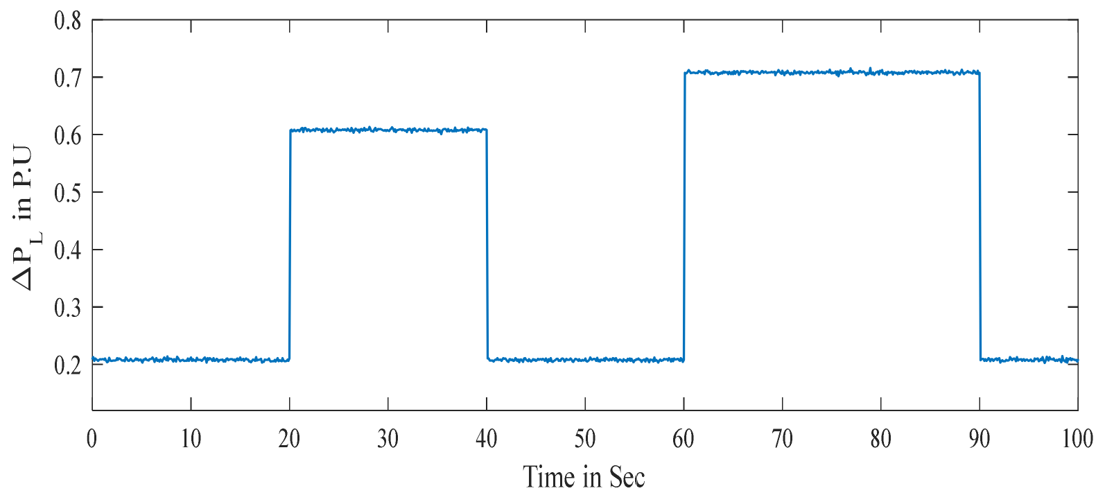
5. Problem-Solving Scenario

Three scenarios have been considered to study the efficacy of the 2DOFTIDF controller.

Case-1: A two-area non-reheat thermal system is considered, and the dynamic performance of the system is studied and contrasted with the recently published DE-optimized TIDF controller [23], PSO-PID, DE-PID, and hBFOA-PSO-PID.

Case-2: Adding nonlinearity as a governor dead band to the system, the dynamic system performances are compared with recent publications.

Case-3: A multi-area multi-unit interconnected system is considered, and the system’s dynamic performance is contrasted with recently published results.

Case-4: Uncertainty conditions with system parameter variation and cross-coupling effect of excitation control and LFC are analyzed.

Case-5: Experimental validation by using OPAL RT.

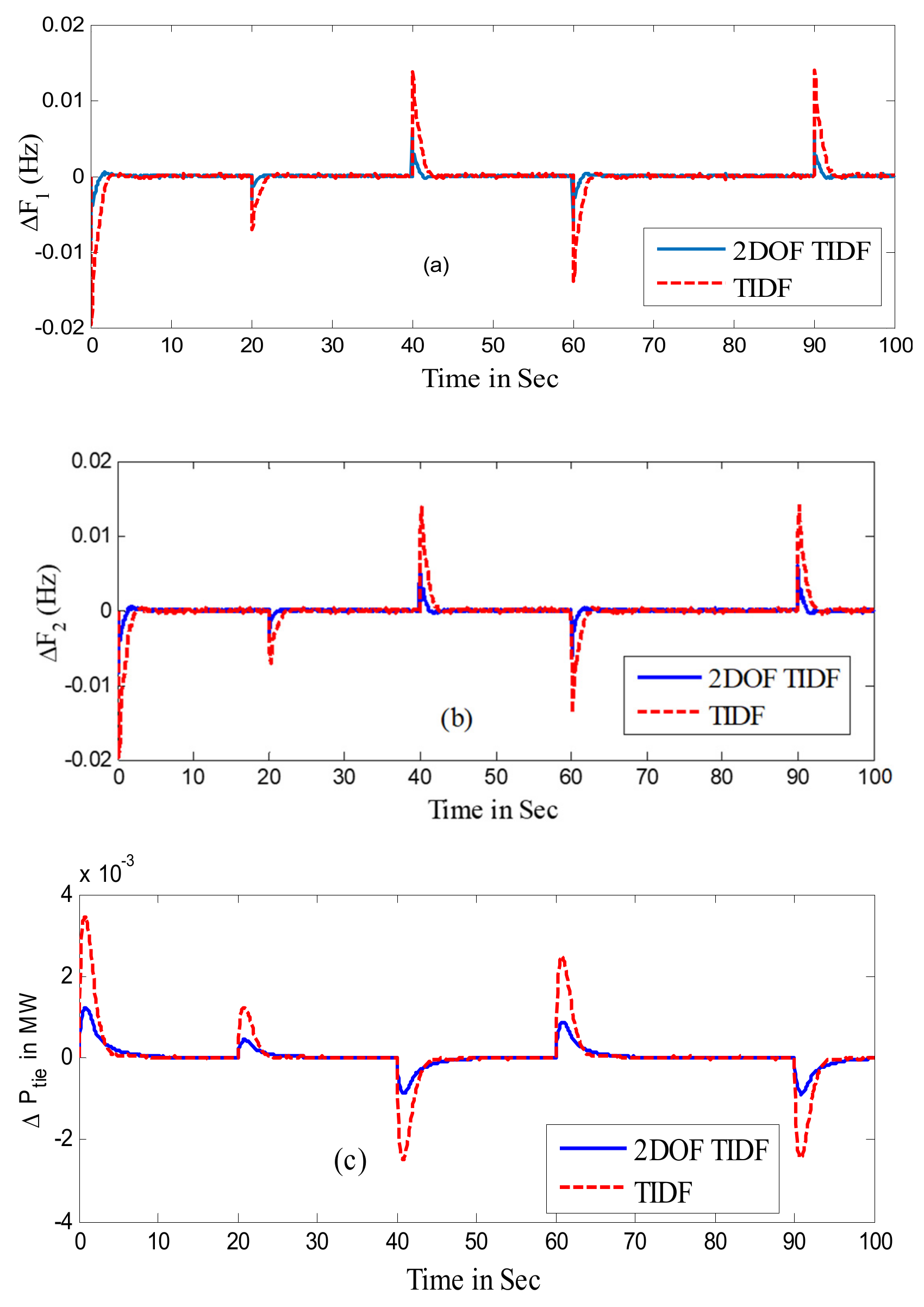
5.1. Case Study Results

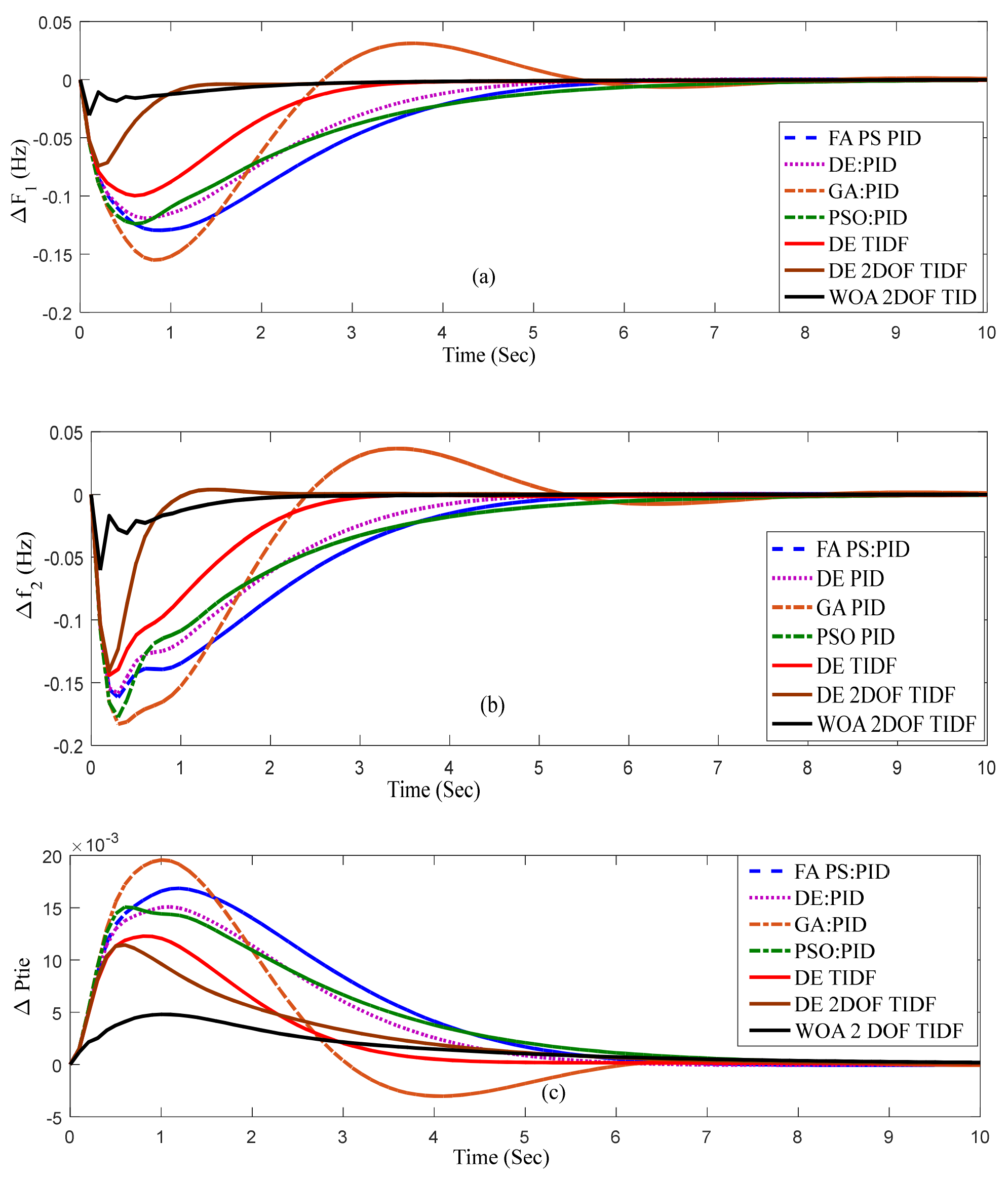
5.1.1. Case-1

For a two-area non-reheat thermal system, a 2DOFTIDF controller was designed for the system. The WOA method was implemented to optimize TIDF and 2DOFTIDF controller parameters. The optimized controller parameters for 10% step load perturbation (SLP) at area-1 with ITAE as the objective function are given as K_t = 1.4024, K_i = 1.8767, K_d = 0.377, N = 230.869, and n = 9.0415 for the TIDF controller and K_t = 3.8815, K_i = 3.9628, K_d = 1.8560, N = 227.7596, n = 9.5667, pw = 1.2430, and dw = 0.4232 for 2DOFTIDF controller with the WOA algorithm. Corresponding dynamic responses for TIDF and 2DOFTIDF controller were obtained and compared with the published results and are shown in Figure 4a–c with SLP of 10% at area-1 and 20% SLP at area-2. The performance index values are given in

Table 1. Comparison of dynamic performances of proposed controller for test system-1.

Optimized Controller	Settling Time (Ts) in Sec			Peak Under Shoot × 10−2			Performance Index
	ΔF1	ΔF2	ΔPtie	ΔF1	ΔF2	ΔPtie
GA-tuned PID [23]	6.93	6.74	4.87	−8.74	−5.22	−2.01	0.4967
PSO-tuned PID [23]	5.30	6.41	5.03	−8.58	−4.36	−1.57	0.4854
FA-tuned PID [23]	4.25	5.49	4.78	−7.88	−4.28	−1.71	0.4714
TLBO-tuned PID [35]	8.53	8.52	5.95	−11.1	14.6	0.099	0.665
DSA PIDF [36]	7.62	6.3	6.94	−13.3	15.4	0	1.09
hGSA-PS PIDF [37]	3.72	4.59	3.61	13.5	19.7	0	0.341
DE-tuned PID [23]	3.58	4.85	4.20	−7.80	−3.92	−1.53	0.3391
DE-tuned TIDF [23]	2.20	3.47	3.01	−6.98	−3.18	−1.23	0.2461
WOA-tuned TIDF	2	2.9	3.0	−6.90	−1.30	−1.14	0.1167
WOA-tuned 2DOF TIDF	1.2	1.5	2.4	−3.07	−6.03	0	0.0734

. Table 1 shows that the WOA-optimized 2DOFTIDF and TIDF controller performance is better than the recently published results for the same system and disturbance. It is clear from Table 1 that the ITAE value is reduced by 76.5% (GA), 75.91% (PSO), 75.24% (FA), 82.45% (TLBO), 89.29% (DSA), 65.77% (hGSA-PS), 65.47% (DE) optimized PID, and 52.58% (DE-TIDF) compared to the proposed WOA-optimized TIDF controller. In addition to that, settling times of ΔF₁ are improved by 71% (GA), 62.27% (PSO), 52.94% (FA), 76.55% (TLBO), 73% (DSA), 46.23% (hGSO-PS), 44.13% (DE) PID, and 9.09% (DE-TIDF) compared to the WOA-tuned TIDF controller. Settling time of ΔF₂ is improved by 56.97% (GA), 54.75% (PSO), 47.17% (FA), 65.96% (TLBO), 53.98% (DSA), 36.8% (hGSA-PS), 40.205% (DE), and 16.42% (DE-TIDF) compared to the WOA-tuned TIDF controller. Settling time of ΔP_Tie is improved by 38.4% (GA), 40.35% (PSO), 37.24% (FA), 49.57% (TLBO), 56.77% (DSA), 16.89% (hGSA-PS), 28.57% (DE)-PID, and 0.33% (DE-TIDF) controller compared to the WOA-optimized TIDF controller. From Figure 4 and Table 1, it is noteworthy that better performance is achieved with the 2DOFTIDF controller compared to TIDF and PID controller in terms of setting time, overshoot, undershoot, and system oscillations. Also, the tuning efficacy of the WOA optimization algorithm was established by comparing the performances with other optimization techniques.

Further improvements in system performance were achieved with the implementation of the 2DOFTIDF controller. Compared to the WOA-tuned TIDF controller, the settling time of ΔF₁, ΔF_2, and ΔP_Tie is improved by 45.45%, 56.77%, and 20.26%, respectively, with the WOA-tuned 2DOFTIDF controller and by 40%, 48.27%, and 20%, respectively, with the DE-tuned TIDF controller. The ITAE value is lessened by 37.10% with the suggested WOA-optimized 2DOFTIDF controller contrasted to the WOA-optimized TIDF controller. Controller output for area-1 U₁ and area-2 U₂ for the 2DOFTIDF controller and TIDF controller are given in Figure 5 for this system with the WOA technique for 10% SLP at area-1 and 20% SLP at area-2. It can be observed from Figure 5 that higher values of overshoot and undershoot for control signals U₁ and U₂ are achieved by the 2DOFTID controller compared to the TIDF controller.

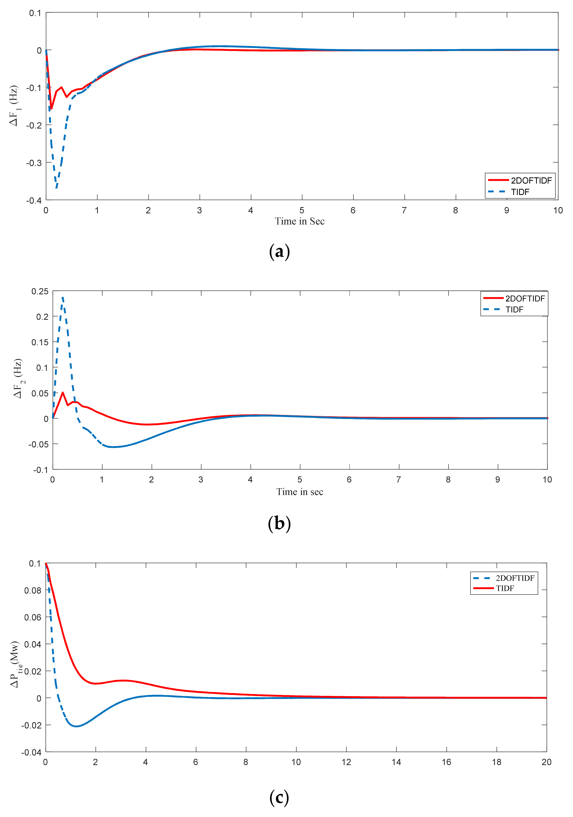
5.1.2. Case-2 Effect of Nonlinearity

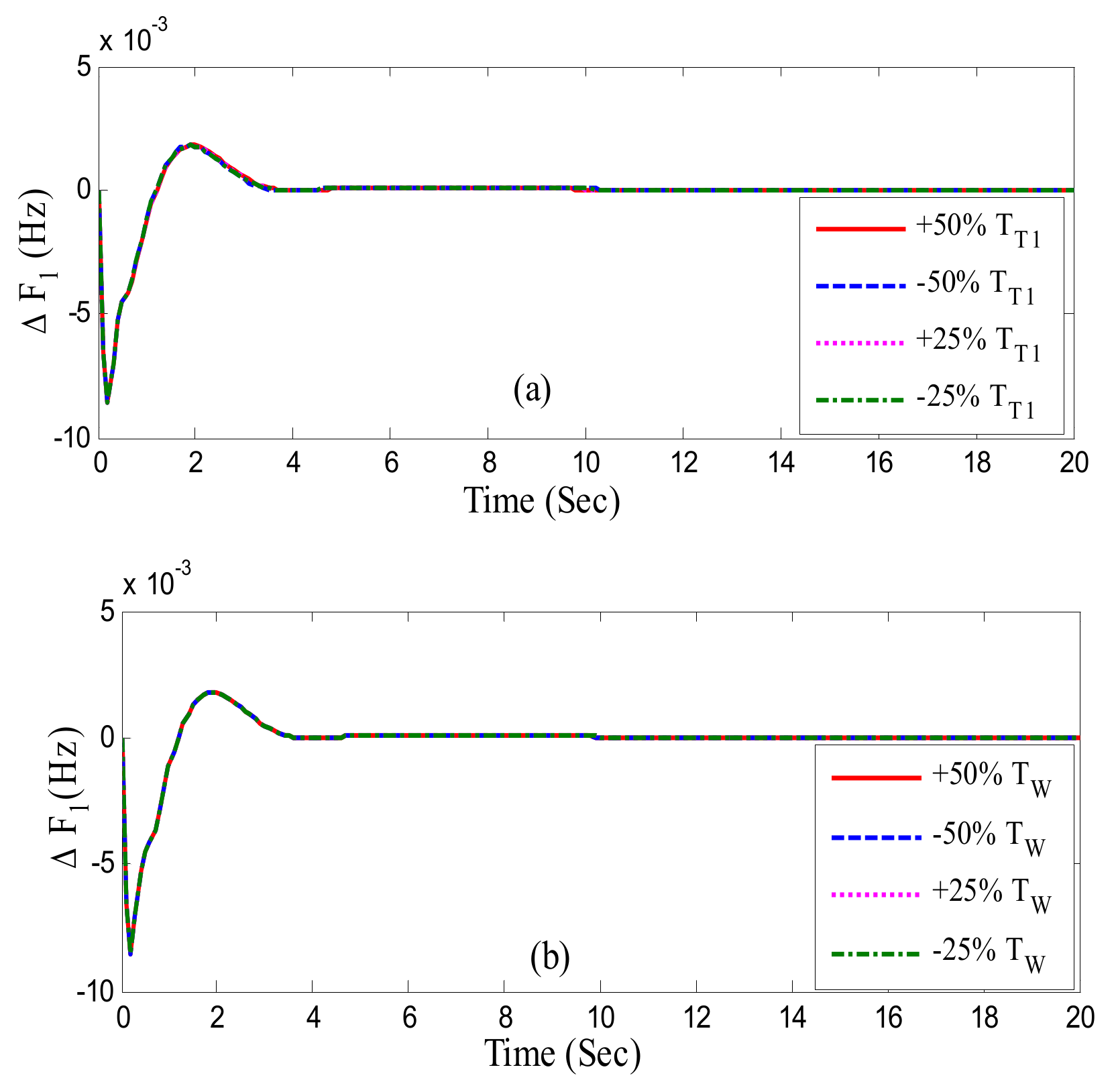
The study was extended to verify the suggested controller’s robustness by adding dead band nonlinearity to a governor. The governor dead band (GDB) is the total range of continuous speed change in which valve position is constant [9]. Due to GDB, for a given change in governor control valves, there is an increase or decrease in speed before the position of the valve changes [38]. The presence of GDB will affect the transient response of the system. In AGC analysis, the dead band effect is certainly important, since small load disturbances are considered. The system with GDB is shown in Figure 6, and an SLP of 1% is applied at area1.

The WOA-optimized TIDF and 2DOFTIDF controller parameters are as follows. TIDF has parameters K_t = 0.6889, K_i = 0.79503, K_d = 0.40963, n = 7.765, and N = 500 and 2DOFTIDF has parameters K_t = 0.5889, K_i = 1.309, K_d = 0.320963, n = 6.765, N = 500, pw = 0.523, and dw = 0.9987. The corresponding dynamic responses with GDB are shown in Figure 7a–c. In order to describe the superiority of the WOA-optimized 2DOFTIDF controller, the system responses were compared with hBFOA-PSO [9]/CRAZYPSO [39]-optimized PI, MFO/WOA [40] optimized DMPI, and TIDF controllers. It is observed from the responses that the proposed controller offers better performance in the presence of nonlinearity. STs, OS, and US for ΔF₁, ΔF₂ and ΔP_tie are embedded in

Table 2. Performance comparison of the proposed controller with GDB.

Optimization Techniques/Controller	ΔF1			ΔF2			ΔPtie			ITAE
	OS (×10−3)	US (×10−3)	ST	OS (×10−3)	US (×10−3)	ST	OS (×10−3)	US (×10−3)	ST
CRAZYPSO: PI [39]	5.0	−31.9	8.56	2.80	−37.1	10.84	0	−9.5	8.65	0.5693
hBFOA-PSO: PI [9]	0.536	−33.7	9.97	4.69	−36.2	10.06	0	−9.1	7.50	0.5059
WOA: DMPI [40]	4.5	−22.1	7.69	1.7	−18.2	8.0	0.263	−5.1	5.14	0.0959
MFO: DMPI [40]	3.3	−23.0	6.99	1.3	−18.5	7.5	0.128	−5.0	5.21	0.175
DE: PID [38]	2.76	−19.3	6.87	1.49	−14.3	4.23	0.114	−3.9	5.91	0.0729
WOA: TIDF	0.374	−14.2	6.05	0	−9.4	6.76	0	−3.1	4.95	0.0688
WOA: 2DOFTIDF	1.6	−9.7	3.2	0.078	−2.7	4.3	0.00012	−2.0	4	0.0214

. From the study of Table 1 and Table 2, it is observed that STs for the system without GDB (ΔF₁ = 1.2 s; ΔF₂ = 1.5 s; ΔP_tie = 2.4 s) are less contrasted to STs (ΔF₁ = 3.2 s; ΔF₂ = 4.3 s; ΔP_tie = 4 s) of the system with nonlinearity. The improvement of ST of the frequency deviation at area-1 is 47.10% (WOA: TIDF), 53.42% (DE: PID), 54.22% (MFO: DMPI), 58.38% (WOA: DMPI), 62.61% (CRAZY PSO: PI), and 67.90% (hBFOA-PSO: PI) with WOA-optimized 2DOFTIDF including GDB. The performance improvement of ST frequency deviation at area-2 is 36.39% (WOA:TIDF), 42.66% (MFO:DMPI), 46.25% (WOA:DMPI), 57.25% (hBFOA-PSO:PI), and 60.33% (CRAZYPSO:PI) with the WOA-tuned 2DOFTIDF controller. Similarly, enhancement in ST of interline power transfer is improved by 19.19% (WOA:TIDF), 32.31% (DE:PID), 23.22% (MFO: DMPI), 22.17% (WOA:DMPI), 46.66% (hBFOA-PSO:PI), and 53.75% (CRAZYPSO: PI) with the WOA-tuned 2DOFTIDF controller. Hence, the above analysis shows that the nonlinear proposed controller offers better performance than the abovementioned controllers.

5.1.3. Case-3

The investigation was further extended to multi-area multi-source systems to verify the efficacy of the suggested WOA-optimized 2DOFTIDF controller. The transfer function model of the system is taken from [31]. Hydro and thermal generation units are considered in each area. A 1.5% SLP was applied in area-1 at t = 0 sec, and the optimization process was repeated 50 times. The best controller parameters obtained in the 50 runs were pw = 1.6426; dw = 1.3370; kt = 5.6215; ki = 4.9773; kd = 1.5785; n = 3.4987; N1 = 132.4083; pw1 = 1.6189; dw1 = 1.2946; kt1 = 4.1064; ki1 = 3.9627; kd1 = 1.8260; n1 = 4.2270; N2 = 36.1646; pw2 = 0.1429; dw2 = 0.1702;kt2 = 3.7908; ki2 = 2.6169; kd2 = 1.6631; n2 = 4.9521; N3 = 123.4507; pw3 = 1.1248; dw3 = 1.6706; kt3 = 4.4553; ki3 = 5.3592; kd3 = 1.0103; n3 = 6.0890; and N4 = 131.9361. Corresponding dynamic responses with the 2DOFTIDF controller are displayed in Figure 8a–c. The ITAE and the settling times in frequency and tie-line power deviations with the WOA-optimized 2DOFTIDF controller were compared with different algorithms and controllers, employing the same objective function provided in

Table 3. Comparison of dynamic performances of proposed controller for test system-2 after 1.5% SLP in area-1.

Optimized Controller	Settling Times (Ts) in Sec			OS × 10−3			Performance Index
	ΔF1	ΔF2	ΔPtie	ΔF1	ΔF2	ΔPtie	ITAE × 10−3
GA: PI [29]	16.03	25.72	9.84	7.8	5.6	1.2	625.8
DA: PI [41]	5.5	7.9	4.9	10.9	5.1	0.51	150
hFA-PS: PI [29]	6.43	8.60	5.98	3.6	0.837	0.0094	228.5
hFA-PS: PID [29]	3.29	5.20	3.92	0.223	0.012	0.067	87.0
DA:PID [41]	2.3	4.4	3.85	0.143	0.011	0.035	45.9
DA: 2DOFPID [41]	1.2	2.7	3.8	0.12	0	0.0022	19.4
WOA: 2DOFSFC [32]	1.7	2	1	1.8	0.10	0.105	24.4
WOA: 2DOFTIDF	0.97	1.4	0.6	0.384	0.004	0.006	6.4

. It is obvious from Table 3 that the lowest value of ITAE is achieved with the proposed WOA-optimized 2DOFTIDF controller compared to GA [29], DA [41], hFA-PS-tuned PI [29], hFA-PS [29], DA [40]-tuned PID, DA-tuned 2DOFPID [41], WOA-tuned 2DOFSFC [32], and WOA-tuned 2DOFPID controllers. The improvements in the ITAE objective function of 98.97% (GA: PI), 95.73% (DA: PI), 97.19% (hFA-PS: PI), 92.64% (hFA-PS: PID), 86.05% (DA: PID), 67.01% (DA: 2DOFPID), and 59.23% (WOA: 2DOFPID) were obtained with the WOA-optimized 2DOFTIDF controller.

It is also clear from Table 3 that the percentage enhancements of ST for Δf₁ with the WOA-optimized 2DOFTIDF controller are 93.94% (GA: PI), 82.36% (DA: PI), 84.91% (hFA-PS:PI), 70.51% (hFA-PS:PID), 57.82% (DA: PID), 19.16% (DA: 2DOFPID), 42.94% (WOA: 2DOFSFC), and 11.81% (WOA:2DOFPID). Similarly, the percentage enhancements of ST for Δf₂ with the WOA-tuned 2DOFTIDF controller were 94.55% (GA: PI), 82.27% (DA: PI), 83.72% (hFA-PS: PI), 73.07% (hFA-PS: PID), 68.18% (DA: PID), 48.14% (DA: 2DOFPID), 30% (WOA: 2DOFSFC), and 33.33% (WOA: 2DOFPID) and the percentage enhancements of ST for ΔP_tie with the WOA-optimized 2DOFTIDF controller were 93.90% (GA: PI), 87.75% (DA: PI), 89.96% (hFA-PS: PI), 84.69% (hFA-PS: PID), 84.41% (DA: PID), 84.21% (DA: 2DOFPID), 40% (WOA: 2DOFSFC), and 25% (WOA: 2DOFPID). Hence, it is detected that the proposed WOA-optimized 2DOFTIDF controller reduced frequency errors in both areas. Therefore, the performance of the WOA-tuned 2DOFTIDF controller is better than the controllers mentioned in the literature.

5.1.4. Case-4

Uncertainty in terms of random load variation with noise (stochastic variation) and parameter variations was applied to test system-1 to test the robustness of the proposed controller. Random load variation with noise was also applied to a two-area non-reheat thermal system in Figure 9. The system performances were analyzed for both the controllers with the WOA technique and are given in Figure 10a–c. As observed in Figure 10, the 2DOFTIDF controller achieved better performance with less oscillation, overshoot, and undershoots than the TIDF controller.

The parameters such as T_H1, T_1, and T_R at area-1 and T_T1 and T_W at area-2 were varied from their normal values in the range of +50% to −50% and +25% to −25% for test system-2. The simulation results of frequency deviation of area-1 corresponding to changed parameters are displayed in Figure 11a–c and Figure 12a,b. System performance indices are accumulated in Table 3. As seen in Figure 11a–c and Figure 12a,b, and

Table 4. Sensitivity analysis.

Parameter Variation	Parameter Variation	Settling Times			Overshoot × 10−3			Obj × 10−3
		ΔF1 (Hz)	ΔF2 (Hz)	ΔPtie	ΔF1 (Hz)	ΔF2 (Hz)	ΔPtie
TH1 at area-1	+50	0.97	1.4	0.6	0.384	0.004	0.006	6.4
	−50	0.98	1.4	0.6	0.384	0.003	0.0067	6.2
	+25	0.97	1.3	0.6	0.384	0.004	0.006	6.4
	−25	0.98	1.3	0.6	0.384	0.005	0.006	6.3
T1 at area-1	+50	0.97	1.4	0.6	0.389	0.005	0.004	6.4
	−50	0.98	1.4	0.6	0.387	0.004	0.003	6.2
	+25	0.99	1.3	0.6	0.384	0.0045	0.003	6.4
	−25	0.98	1.4	0.6	0.384	0.004	0.004	6.4
TR at area-1	+50	0.99	1.4	0.55	0.384	0.0045	0.004	6.3
	−50	0.97	1.3	0.6	0.384	0.0045	0.006	6.4
	+25	0.97	1.4	0.59	0.384	0.0043	0.056	6.3
	−25	0.97	1.4	0.6	0.384	0.004	0.006	6.4
TT1 at area-2	+50	0.97	1.4	0.6	0.384	0.004	0.0063	6.4
	−50	0.99	1.3	0.56	0.384	0.044	0.0067	6.3
	+25	0.99	1.4	0.6	0.384	0.004	0.0064	6.4
	−25	0.97	1.4	0.6	0.384	0.004	0.0063	6.3
TW at area-2	+50	0.97	1.3	0.58	0.384	0.045	0.0069	6.4
	−50	0.98	1.4	0.6	0.384	0.0045	0.0067	6.3
	+25	0.97	1.3	0.6	0.384	0.004	0.0068	6.4
	−25	0.98	1.3	0.6	0.384	0.004	0.0065	6.1

, there are fewer variations in system performances with the parameter variations. The critical examination of the results reveals that the proposed controller offers robust behavior and there is no need to reset for wide variations in the system’s parameters.

To show the coupling effect of excitation control and LFC, a step voltage perturbation (SPV) of 1% was applied as a disturbance at area-1 at t = 0, and the system performances were studied for the TIDF and 2DOFTIDF controllers for the same controller parameters as obtained previously. System dynamic performances are shown in Figure 13a–c. As seen in Figure 13, the performance of the 2DOFTIDF controller is better compared to the TIDF controller. With the same controller parameters, by applying step voltage change, the PS regains its stability, exhibiting the robust action of the controller.

It is observed that the proposed WOA-optimized 2DOFTIDF controller will lessen frequency errors in both areas for two test cases and with nonlinearity also. For two different test cases, the performance of the 2DOFTIDF controller was found to be better than the DE-optimized TIDF, hFA-PS-optimized PID and GA, and ZN-optimized PI controller. The proposed controller is also robust enough to manage random load variation with noise and parameter variations. The cross-coupling effect of excitation voltage and LFC was compared for the TIDF and 2DOFTIDF controllers. These subjects express that this controller can be planned to control any interconnected PS with improved system performance.

For the same considered test system-1 in [42], the superiority of the 2DOF TIDF controller is mentioned in the following

Table 5. Comparison table with latest work.

Controller	Controller Settling Time (Ts) in Sec
	∆F1	∆F2	∆Ptie
WOA 2DOF TIDF	1.2	1.5	2.4
Adaptive Differential Evolution 2DOF TIDF	2.54	3.28	1.05

.

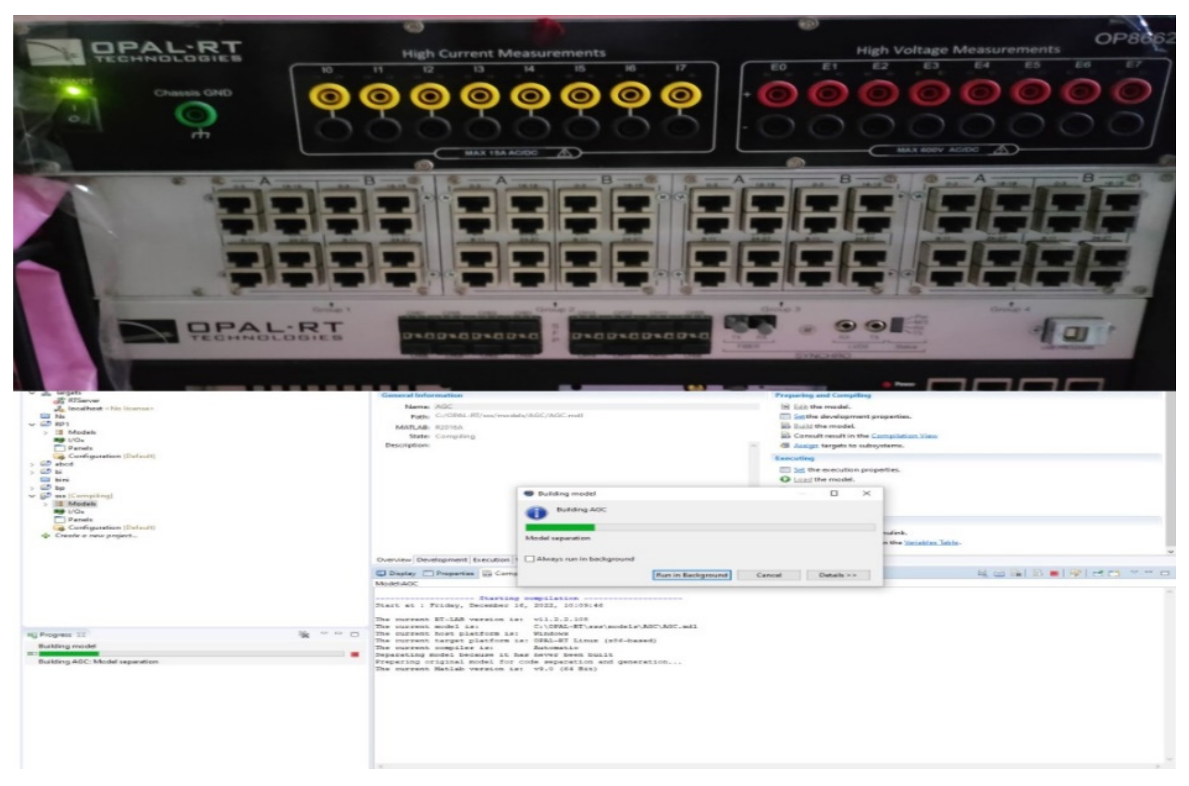
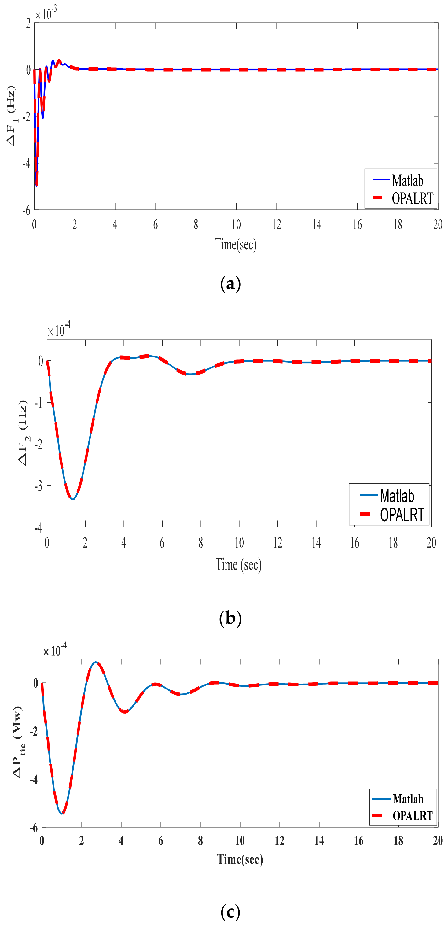
5.1.5. Case-5 Experimental Validation by Using OPAL RT

As shown in Figure 14, the hardware-in-the-loop (HIL) simulation approach based on OPAL-RT is used for experimental validation of the suggested control approach. The suggested approach is confirmed to work in a real-time setting without overruns by using the real-time HIL approach, which additionally includes mistakes and delays that are missing from the traditional off-line simulations.

The HIL setup consists of a PC acting as a command station where MATLAB (Burla, India)/Simulink-based codes are generated for execution on the OPAL-RT, an OPAL-RT real-time simulator (RTS), which simulates the power system models of test systems, and a router to connect all the setup devices in a single sub-network.

Figure 15 displays the RTS and MATLAB/Simulink results for all test systems. Figure 15a–c shows that for test systems, the RTS findings match the MATLAB/Simulink results exactly.

6. Conclusions

A novel controller is formed by hybridizing two-degree freedom with a tilt-integral-derivative with filter (2DOFTIDF), which is intended and executed for the AGC problem. The best controller parameter is obtained with the whale optimization technique. To test the efficiency of the suggested methodology, different test systems are investigated. The proposed approach was compared with DE-TIDF, hGSA-PS-PIDF/PI, DA-PI/PID/2DOFPID, WOA-2DOFSFC, WOA-DMPI, and WOA-TIDF controllers, and better dynamic performances were achieved with the WOA-optimized 2DOFTIDF controller. The robustness of the controller and the cross-coupling effect of AVR and LFC were also analyzed. However, it can be concluded that the proposed controller was successfully employed for the load frequency control problem. For a two-area non-reheat thermal system, settling times of ΔF₁, ΔF₂ and ΔP_Tie are improved by 40%, 48.27%, and 20% with the WOA 2DOFTIDF controller compared to the WOA TIDF controller. After applying GDB nonlinearity to the system, the frequency deviations were improved by 47.10%, 36.39%, and 19.19% with the WOA 2DOFTIDF controller compared to the WOA TIDF controller. With the proper design of the controller, it can also be applied to any engineering problem.

References

1. Kundur, P. Power System Stability and Control.; Tata McGraw-Hill: New Delhi, India, 2009; 8th reprint. [Google Scholar]
2. Abdelaziz, A.Y.; Ali, E.S. Static VAR Compensator Damping Controller Design Based on Flower Pollination Algorithm for a Multi-machine Power System. Electr. Power Compon. Syst. 2015, 43, 1268–1277. [Google Scholar] [CrossRef]
3. Mansouri, S.A.; Nematbakhsh, E.; Ahmarinejad, A.; Jordehi, A.R.; Javadi, M.S.; Marzband, M. A hierarchical scheduling framework for resilience enhancement of decentralized renewable-based microgrids considering proactive actions and mobile units. Renew. Sustain. Energy Rev. 2022, 168, 112854. [Google Scholar] [CrossRef]
4. Mansouri, S.A.; Nematbakhsh, E.; Jordehi, A.R.; Tostado-Véliz, M.; Jurado, F.; Leonowicz, Z. A risk-based bi-level bidding system to manage day-ahead electricity market and scheduling of interconnected microgrids in the presence of smart homes. In Proceedings of the 2022 IEEE International Conference on Environment and Electrical Engineering and 2022 IEEE Industrial and Commercial Power Systems Europe (EEEIC/I&CPS Europe), Prague, Czech Republic, 28 June 2022; pp. 1–6. [Google Scholar]
5. Elgerd, O.I. Electric Energy Systems Theory. An Introduction; TMH: New Delhi, India, 1983. [Google Scholar]
6. Bevrani, H. Robust Power System Frequency Control; Springer: New York, NY, USA, 2009. [Google Scholar]
7. Saikia, L.C.; Nanda, J.; Mishra, S. Performance comparison of several classical controllers in AGC for multi-area interconnected thermal system. Int. J. Electr. Power Energy Syst. 2011, 33, 394–401. [Google Scholar] [CrossRef]
8. Shabani, H.; Vahidi, B.; Ebrahimpour, M. A robust PID controller based on imperialist competitive algorithm for load-frequency control of power systems. ISA Trans. 2012, 52, 88–95. [Google Scholar] [CrossRef] [PubMed]
9. Panda, S.; Mohanty, B.; Hota, P.K. Hybrid BFOA–PSO algorithm for automatic generation control of linear and nonlinear interconnected power. Appl. Soft Comput. 2013, 13, 4718–4730. [Google Scholar] [CrossRef]
10. Madasu, S.D.; Kumar, M.S.; Singh, A.K. A flower pollination algorithm based automatic generation control of interconnected power system. Ain Shams Eng J. 2016, 9, 1215–1224. [Google Scholar] [CrossRef] [Green Version]
11. Abdelaziz, A.Y.; Ali, E.S. Load Frequency Controller Design via Artificial Cuckoo Search. Electric Power Components and Systems. Electr. Power Compon. Syst. 2015, 44, 90–98. [Google Scholar] [CrossRef]
12. Abo-Elyousr, F.K.; Abdelaziz, A.Y. A Novel Modified Robust Load Frequency Control for Mass-less Inertia Photovoltaics Penetrations via Hybrid PSO-WOA Approach. Electr. Power Compon. Syst. J. 2019, 47, 1744–1759. [Google Scholar] [CrossRef]
13. Saikia, L.C.; Sinha, N.; Nanda, J. Maiden application of bacterial foraging based fuzzy IDD controller in AGC of a multi-area hydrothermal system. Int. J. Electr. Power Energy Syst. 2013, 45, 98–106. [Google Scholar] [CrossRef]
14. Khuntia, S.R.; Panda, S. Simulation study for automatic generation control of a multi-area power system by ANFIS approach. Appl. Soft Comput. 2012, 12, 333–341. [Google Scholar] [CrossRef]
15. Mohanty, B. TLBO optimized sliding mode controller for multi-area multi-source nonlinear interconnected AGC system. Int. J. Electr. Power Energy Syst. 2015, 73, 872–881. [Google Scholar] [CrossRef]
16. Yesil, E. Interval type-2 fuzzy PID load frequency controller using big-bang big-crunch optimization. Appl. Soft Comput. 2014, 15, 100–112. [Google Scholar] [CrossRef]
17. Hiroi, K.; Togari, Y. Two Degrees of Freedom PID Algorithm with Compound Filter. Trans. Soc. Instrum. Control. Eng. 1991, 27, 402–408. [Google Scholar] [CrossRef] [Green Version]
18. Sahu, R.K.; Panda, S.; Rout, U.K. DE optimized parallel 2-DOF PID controller for load frequency control of power system with governor dead-band nonlinearity. Int. J. Electr Power Energy Syst. 2013, 49, 19–33. [Google Scholar] [CrossRef]
19. Elsaied, M.M.; Hameed, W.H.A.; Hasanien, H.M. Frequency stabilization of a hybrid three-area power system equipped with energy storage units and renewable energy sources. IET Renew. Power Gener. 2022, 16, 3267–3286. [Google Scholar] [CrossRef]
20. Daraz, A.; Malik, S.A.; Waseem, A.; Azar, A.T.; Haq, I.U.; Ullah, Z.; Aslam, S. Automatic Generation Control of Multi-Source Interconnected Power System Using FOI-TD Controller. Energies 2021, 14, 5867. [Google Scholar] [CrossRef]
21. Debbarma, S.; Saikia, L.C.; Sinha, N. Automatic generation control using two degrees of freedom fractional order PID controller. Int. J. Electr. Power Energy Syst. 2014, 58, 120–129. [Google Scholar] [CrossRef]
22. Lurie, B.J. Three-Parameter Tunable Tilt-Integral Derivative (TID) Controller. US Patent US5371670, 6 December 1994. [Google Scholar]
23. Sahu, R.K.; Panda, S.; Biswal, A.; Sekhar, G.C. Design and analysis of tilt integral derivative controller with filter for load frequency control of multi-area interconnected power systems. ISA Trans. 2016, 61, 251–264. [Google Scholar] [CrossRef]
24. Sain, D.; Swain, S.K.; Mishra, S.K. TID and I-TD controller design for magnetic levitation system using genetic algorithm. Perspect. Sci. 2016, 8, 370–373. [Google Scholar] [CrossRef] [Green Version]
25. Asadollahi, M.; Rikhtegar ghiasi, A.; Dehghani, H. Excitation control of a synchronous generator using a novel fractional-order controller. IET Gen. Tran. Dist. 2015, 9, 2255–2260. [Google Scholar] [CrossRef]
26. Abd-Elazim, S.M.; Ali, E.S. Load frequency controller design via BAT algorithm for nonlinear interconnected power system. Int. J. Electr. Power Energy Syst. 2016, 77, 166–177. [Google Scholar] [CrossRef]
27. Guha, D.; Roy, P.K.; Banerjee, S. Load frequency control of large scale power system using quasi-oppositional grey wolf optimization algorithm. Eng. Sci. Technol. Int. J. 2016, 19, 1693–1713. [Google Scholar] [CrossRef] [Green Version]
28. Dash, P.; Saikia, L.C.; Sinha, N. Comparison of performance of several cuckoo search algorithm based 2DOF controllers in AGC of multi-area thermal system. Int. J. Electr. Power Energy Syst. 2014, 55, 429–436. [Google Scholar] [CrossRef]
29. Sahu, R.K.; Panda, S.; Padhan, S. A hybrid firefly algorithm and pattern search technique for automatic generation control of multi area power systems. Int. J. Electr. Power Energy Syst. 2015, 64, 9–23. [Google Scholar] [CrossRef]
30. Mohanty, B. Performance analysis of moth flame optimization algorithm for AGC analysis. Int. J. Model. Simul. 2018, 39, 73–87. [Google Scholar] [CrossRef]
31. Mirjalili, S.; Lewis, A. Whale Optimization Algorithm. Adv. Eng. Softw. 2016, 95, 51–67. [Google Scholar] [CrossRef]
32. Hasanien, H.M. Whale optimization algorithm for automatic generation control of interconnected modern power system including renewable energy sources. IET Gen. Tran. Dist. 2018, 12, 607–614. [Google Scholar] [CrossRef]
33. Kumar, C.S.; Rao, R.S.; Cherukuri, S.K.; Rayapudi, S.R. A Novel Global MPP Tracking of Photovoltaic System based on Whale Optimization Algorithm. Int. J. Renew. Energy Dev. 2016, 5, 225–232. [Google Scholar] [CrossRef]
34. Tepljakov, A.; Petlenkov, E.; Belikov, J. FOMCON: A MATLAB Toolbox for Fractional-order System Identification and Control. Int. J. Microelectron. Comput. Sci. 2011, 2, 51–62. [Google Scholar]
35. Sahu, R.K.; Panda, S.; Rout, U.K.; Sahoo, D.K. Teaching learning based optimization algorithm for automatic generation control of power system using 2-DOF PID controller. Int J Elect Power Energy Syst. 2016, 77, 287–301. [Google Scholar] [CrossRef]
36. Guha, D.; Roy, P.K.; Banerjee, S. Study of differential search algorithm based automatic generation control of an interconnected thermal-thermal system with governor dead band. Appl. Soft Comput. 2017, 52, 160–175. [Google Scholar] [CrossRef]
37. Sahu, R.K.; Panda, S.; Padhan, S. A novel hybrid gravitational search and pattern search algorithm for load frequency control of nonlinear power system. Appl. Soft Comput. 2015, 29, 310–327. [Google Scholar] [CrossRef]
38. Mohanty, B.; Panda, S.; Hota, P.K. Differential evolution algorithm based Automatic generation control for interconnected power systems with nonlinearity. Alex. Eng. J. 2014, 53, 537–552. [Google Scholar] [CrossRef] [Green Version]
39. Gozde, H.; Taplamacioglu, M.C. Automatic generation control application with craziness based particle swarm optimization in a thermal power system. Int. J. Elect. Power Energy Syst. 2011, 33, 8–16. [Google Scholar] [CrossRef]
40. Simhadri, K.S.; Mohanty, B. Performance analysis of dual-mode PI controller using quasi-oppositional whale optimization algorithm for load frequency control. Int. Trans. Elect Energy Syst. 2019, 30, e12159. [Google Scholar] [CrossRef]
41. Simhadri, K.; Mohanty, B.; Rao, U.M. Optimized 2DOF PID for AGC of multi-area power system using dragonfly algorithm. In Applications of Artificial Intelligence Techniques in Engineering. Advances in Intelligent Systems and Computing; Malik, H., Srivastava, S., Sood, Y., Ahmad, A., Eds.; Springer: Singapore, 2019; Volume 698, pp. 11–22. [Google Scholar]
42. Chintu, J.M.R.; Sahu, R.K.; Panda, S. Design and analysis of two degree of freedom tilt integral derivative controller with filter for frequency control and real time validation. J. Electr. Eng. 2020, 71, 388–396. [Google Scholar] [CrossRef]
43. Zhao, J.; Gao, Z.M. The bat algorithm and its parameters. In Proceedings of the 4th International Conference on Electronic, Communications and Networks (CECNet2014), Beijing, China, 12–15 December 2014; CRC Press: Boca Raton, FL, USA, 2014; pp. 1323–1326. [Google Scholar]
44. Kim, C.-H.; Khurshaid, T.; Wadood, A.; Farkoush, S.G.; Rhee, S.-B. Gray wolf optimizer for the optimal coordination of directional overcurrent relay. J. Electr. Eng. Technol. 2018, 13, 1043–1051. [Google Scholar]
Figure 1. Two areas of non-reheat thermal PS [18].
Sustainability 15 01515 g001
Figure 2. Structure of two−degree freedom control.
Sustainability 15 01515 g002
Figure 3. The control structure of 2DOF−TIDF.
Sustainability 15 01515 g003
Figure 4. (ac) Comparison of dynamic responses of test system-1 (a)ΔF1 vs. Time, (b) ΔF2 vs. Time, (c) ΔPtie vs. Time.
Sustainability 15 01515 g004
Figure 5. TIDF and 2DOF TIDF controller outputs at area−1 with 10% Step Load Perturbation (SLP) and at area−2 with 20% SLP.
Sustainability 15 01515 g005
Figure 6. Two areas of the non−reheat thermal system with GDB [18].
Sustainability 15 01515 g006
Figure 7. (ac) Responses of test system−1 with GDB nonlinearity (a) ΔF1 vs. Time, (b) ΔF2 vs. Time, (c) ΔPtie vs. Time.
Sustainability 15 01515 g007
Figure 8. (ac) Comparison of dynamic responses of test system-2 with 2DOF TIDF controller.
Sustainability 15 01515 g008
Figure 9. Random load variation with noise ΔPL vs. Time.
Sustainability 15 01515 g009
Figure 10. (ac) Dynamic system performances with random load variation with noise.
Sustainability 15 01515 g010
Figure 11. (ac). Frequency deviation of area−1 with 1% step load change in area-1 with varying Tg1, T1, TR.
Sustainability 15 01515 g011
Figure 12. (a,b). Frequency deviation of area−1 with 1% step load change in area-1 with varying TT1 and TW at area-2 for test system-2.
Sustainability 15 01515 g012
Figure 13. Comparison of dynamic responses of test system−1 with 2DOFTIDF and TIDF controllers with 1% SPV (a) ΔF1 vs. Time, (b) ΔF2 vs. Time, (c) ΔPtie vs. Time.
Sustainability 15 01515 g013
Figure 14. Experimental setup using OPAL-RT.
Sustainability 15 01515 g014
Figure 15. Comparison of real−time simulation results with MATLAB/Simulink results. (a) ΔF1 vs. Time, (b) ΔF2 vs. Time, (c) ΔPtie vs. Time.
Sustainability 15 01515 g015