Spatiotemporal Responses of Vegetation to Hydroclimatic Factors over Arid and Semi-arid Climate

Abstract

Understanding the dynamics of vegetative greenness and how it interacts with various hydroclimatic factors is crucial for comprehending the implications of global climate change. The present study utilized the MODIS-derived normalized difference vegetation index (NDVI) to understand the vegetation patterns over 21 years (2001–2021) in Rajasthan, India. The rainfall, land surface temperature (LST), and evapotranspiration (ET) were also analyzed. The changes, at a 30 m pixel resolution, were evaluated using Mann–Kendall’s trend test. The results reveal that the NDVI, ET, and rainfall had increasing trends, whereas the LST had a decreasing trend in Rajasthan. The NDVI increased for 96.5% of the total pixels, while it decreased for 3.4% of the pixels, of theh indicates vegetation improvement rather than degradation. The findings of this study provide direct proof of a significant reduction in degraded lands throughout Rajasthan, particularly in the vicinity of the Indira Gandhi Canal command area. Concurrently, there has been a noticeable expansion in the cultivated land area. The trend of vegetation decline, particularly in the metro cities, has occurred as a result of urbanization and industrialization. In contrast to the LST, which has a decreasing gradient from the western to eastern portions, the spatial variability in the NDVI, ET, and rainfall have decreasing gradients from the southern and eastern to western regions. The results of correlations between the vegetative indices and hydroclimatic variables indicate that the NDVI has a strong positive correlation with ET (r² = 0.86), and a negative correlation with LST (r² = −0.55). This research provides scientific insights into vegetation change across Rajasthan, and may help the state to monitor vegetation changes, conserve ecosystems, and implement sustainable ecosystem management.

1. Introduction

Vegetation is an integral part of the terrestrial ecosystem and is an essential component of the biosphere [1]. Vegetation is a critical element of soil–water–plant–atmospheric systems, having a considerable influence on the global energy budget, as well as hydrological, terrestrial carbon, and biogeochemical cycles from a local-to-global scale over seasonal, annual, and decadal periods [2,3,4]. Vegetation dynamics can act as an essential parameter for changes in the environment, including climatic and hydrological parameters like temperature, precipitation, evapotranspiration (ET), and land surface temperature, because it has a clear relationship with climate change [5,6].

In recent decades, vegetation–climate interactions have gained much attention due to global climate change [7,8,9,10,11,12,13]. However, past studies have been carried out worldwide by various researchers to understand vegetation dynamics using the vegetation index. Sur et al. [14] used 17 years (2000–2016) of normalized difference vegetation index (NDVI) datasets to characterize the spatiotemporal change in vegetation over the western part of Rajasthan. Mariano et al. [15] analyzed land degradation and drought events using the moderate resolution imaging spectroradiometer (MODIS)-leaf-area index, albedo, and evapotranspiration images for northeastern Brazil for 2002–2016. Many researchers have studied the changes in vegetation patterns on the Mongolian Plateau, and their responses to climatic factors and human activities [16,17,18,19]. Globally, the trend of vegetation dynamics and its interaction with associated drivers, such as precipitation, temperature, and evapotranspiration, have been studied using satellite-based products [20,21,22,23,24].

Ground observation is currently the most precise method for capturing local vegetation conditions. However, due to the limited number and uneven distribution of ground stations, it is challenging to use ground observation directly on a regional or global scale [19]. The utilization of long-term satellite data enables the better monitoring and evaluation of surface vegetation dynamics in relation to climate change on different spatiotemporal scales [25,26]. The land surface vegetation can be effectively characterized by using satellite-derived vegetation indices, such as the normalized difference vegetation index (NDVI) and the enhanced vegetation index (EVI) [23]. Among several vegetation indices, the NDVI is the most extensively used index as a proxy for monitoring vegetation dynamics across the world [27,28,29,30]. Globally, many researchers have explored the changes in vegetation dynamics using this remote sensing-based vegetation index for arid and semi-arid regions [14,15,24,31]. The simplicity of its calculations, its availability at several temporal and spatial scales, and its ability to eliminate noises arising from illumination conditions, topography, clouds, and other atmospheric conditions, make the NDVI an essential index for monitoring vegetation dynamics [32]. In addition, past studies primarily focused on analyzing vegetation trends using a single index. Moreover, there has been relatively little research in the Indian context, particularly in Rajasthan, highlighting vegetation–hydroclimatic interactions. Therefore, an in-depth analysis of vegetation dynamics and its response to climate change in Rajasthan still needs further clarification. This present study focused mainly on the vegetation indices’ annual and seasonal variations, and their relationship with hydroclimatic variables from 2001 to 2021. We hypothesized that Rajasthan state had undergone a vegetative- greening or -browning trend due to changes in climatic factors, the intensification of canal irrigation, and urbanization. The goals of the present study were as follows: (1) to evaluate the seasonal and annual variations in the NDVI and hydroclimatic factors in Rajasthan during the past 21 years; and (2) to analyze trends at the pixel level using the Mann–Kendall (MK) test. This study will help to analyze the root causes behind drought phenomenon, the restoration of degraded lands, and ecosystem services in the study area.

2. Materials and Methods

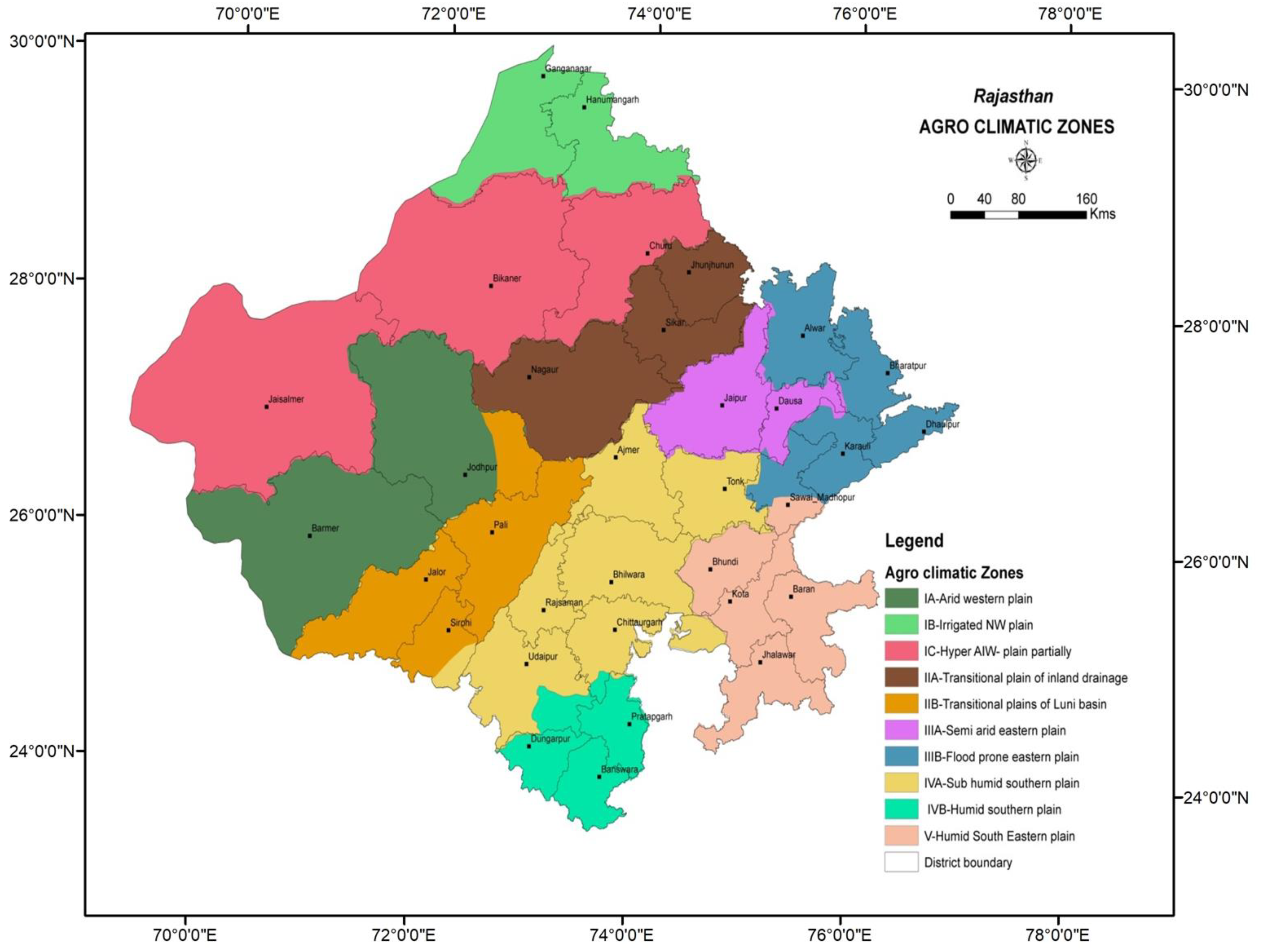
2.1. Study Area

The current study was carried out in Rajasthan state, in western India; a peculiarly hot spot prone to substantial changes induced by climate change and anthropogenic modifications. Rajasthan is located in northwestern India and lies between the latitudes of 23°30′ and 30°11′ N and the longitudes of 69°29′ and 78°17′ E. Geographically, it occupies a 342,239 km² area, which covers almost 10.4% of the country’s total geographical location, making it India’s largest state. Rajasthan has a diverse topography, with the Aravalli Hills in the center (which extends from the northeast to the southwest), the Thar Desert in the northwest, sand plains in the northeast, and a plateau in the southeastern part. The climate in Rajasthan is characterized by insufficient (480–750 mm) and highly erratic rainfall distribution, high evaporation losses, low humidity values, strong winds, and extreme air temperature values. The Aravalli Hills significantly impact Rajasthan’s climate, due to its orientation parallel to the southwest monsoon. The eastern slope of the Aravalli Hills is hit by the Arabian Sea branch of the southwest monsoon so it receives adequate rainfall, while the northwestern portion remains dry. However, moderate-to-highly humid climatic conditions prevail in the southeastern parts of the state.

Ten agro-climatic zones (ACZ) are present in the state: (i) the arid western plain; (ii) the irrigated northwestern plains; (iii) the hyper-arid partially irrigated western plain; (iv) the transitional plain with inland drainage; (v) of thethe transitional plain of the Luni Basin; (vi) the semi-arid eastern plain; (vii) the flood-prone eastern plains; (viii) the sub-humid southern plains; (ix) the humid southern plains; and (x) the humid southeastern plains (Figure 1). The hyper-arid partially irrigated western plain and the arid western plain have harsh climatic conditions with inadequate rainfall and low vegetation cover. The soil of these zones are characterized by dunes and aeolian soil. The humid southern plains and the humid southeastern plains climatic zones receive good rainfall and have high vegetation coverage. The state has two main important cropping seasons: Kharif and Rabi. In Kharif, crops are sown between June and July and are reaped between September and October; in Rabi, crops are sown between October and November and are reaped between March and April. The net sown area of Rajasthan is 18.13 Mha, which is about 53% of the TGA, while fallow land and forest cover 3.62 Mha (11%) and 2.77 M ha (8%), respectively. The other remaining areas fall under non-agricultural uses, barren land, permanent pasture, and other grazing land. Out of 20 million hectares of cultivated area, only 20% is irrigated because the state has only 1% of the country’s total water resources [33].

2.2. Data Set

Data from high-resolution satellite images are excellent sources for monitoring a large area’s mapping and time-series analysis. Taking advantage of the accessibility of long-term satellite datasets, we have chosen four key parameters with which to characterize the spatiotemporal variation in the vegetation–hydroclimatic interactions. The current study utilized the MODIS-derived NDVI to comprehend the vegetation patterns from 2001 to 2021. Three hydroclimatic factors were also used to understand the climatic variation during 2001–2021 (Figure 2). The various datasets and their specifications are given in

Table 1. The dataset used in this study and its specifications.

S. No.	Dataset	Variable	Unit	Temporal Resolution	Spatial Resolution	Period
1	MODIS MOD13Q1	NDVI	-	16 days	250 m	2001–2021
2	CHIRPS	Rainfall	mm	Daily	5 km	2001–2021
3	MODIS MOD11A2	LST	°C	8 days	1 km	2001–2021
4	MODIS MOD16A2GF	ET	kg/m2/8 d	8 days	500 m	2001–2021

.

2.3. Downloading and Processing of Satellite Data

2.3.1. NDVI

The NDVI data from the NASA Land Processes Distributed Active Archive Center’s MODIS products (MOD13Q1) were used in the present study. The best pixel values from the acquisitions made by satellites over 16 days were selected by algorithms using the primary criteria of low clouds, small view angles, and maximum NDVI. In the current study, the NDVI product of MODIS MOD13Q1 was downloaded from Google Earth Engine for the 21 years (2001–2021). The NDVI time-series data were temporally smoothed using the Savitzky–Golay filter (SGF) [34]. The SGF uses a weighted least-squares regression to fit a polynomial function. The data sets were reprojected from the geographic coordinates system to a UTM 43 coordinate system. Furthermore, the datasets were resampled to 30 m cell size using bilinear interpolation in ArcGIS (10.5) [35].

2.3.2. Rainfall

In the present study, we used 5 km spatial resolution rainfall data from the climate-hazards group infrared precipitation with station data (CHIRPS)-based rainfall products. The datasets were downloaded using Google Earth Engine for the 21 years (2001–2021). The mean monthly rainfall was computed by taking the mean of the respective month for the 21 years (2001–2021). Similarly, the total annual rainfall was computed by calculating the sum of all the images for the individual year.

2.3.3. Land Surface Temperature

In this study, the MODIS MOD11A2 LST product was downloaded from Google Earth Engine for the 21 years (2001–2021). The data were further converted into °C [36,37] using the following formula:

$$\mathrm{L}\mathrm{S}\mathrm{T}=0.02\times \mathrm{D}\mathrm{N}-273.15$$

The mean monthly LST values were computed by calculating each month’s mean for 2001–2021. Similarly, the mean annual LST was computed by calculating the mean of all the images of the respective year.

2.3.4. Evapotranspiration (ET)

The evapotranspiration data were obtained from MODIS, and were highly correlated with the ET observations of the Indian conditions [38]. Based on the Penman–Monteith equation, the MOD16 data-product collection algorithm incorporates inputs from the daily reanalysis of meteorological data and MODIS data products, like vegetation dynamics, land cover, and albedo. The pixel values for the ET layer were calculated by adding data from an 8-day composite period. The data product MOD16A2GF was downloaded from Google Earth Engine from 2001 to 2021 using the following steps: (i) the monthly ET was computed by aggregating the 8-day composite images within the respective month of the particular year. (ii) After that, the long-term (21 years) mean monthly ET for each month was computed by calculating the mean of the respective month. (iii) Similarly, the total annual ET was calculated by aggregating the monthly ETs for the respective year.

2.4. Trend Analysis

We used the nonparametric MK test and Sen’s slope estimator [39,40] to assess the significant trends and magnitudes, respectively. Hamed and Rao (1998) [41] introduced a modified version of the MK test to consider the effect of autocorrelation on the data. They proposed a correction of the variance for the adequate number of observations. The null hypothesis (H0) of no trend, and the alternative hypothesis of there being a trend, were tested at a 5% level of significance. The trend tests were implemented using R 4.2.1 software.

Four factors (NDVI, LST, ET, and rainfall) were downloaded using Google Earth Engine for the 21 years (2001–2021). All these input layers had varying resolutions (Table 1). To harmonize the datasets, all the raster layers were resampled to 30 m using a bilinear resampling method. After that, these datasets were used for the MK test. First, all the images were stacked in one raster in ascending order of year. Then, the MK test was implemented using a raster and the Kendall function from the spatialEco package.

Methodology Description:

The computational procedure for the MK test for the time-series data, $y_1, y_2, y_3, \dots , y_n$, was as follows:

Step 1: Calculate all-possible differences of $y_i-y_j$, where $i>j$, i.e., $\frac{n(n-1)}{2}$ for the given time-series data. The differences are

$$y_2-y_1, y_3-y_2, \dots , y_n-y_{n-1}$$

Step 2: Determine the sign of all the differences $\left(y_i-y_j\right)$.

Step 3: Assign numerical values to the sign differences. The assignment rule is as follows:

$$sign \left(y_i-y_j\right)=\left\{\begin{array}{c}1;if \left(y_i-y_j\right)>0\\ 0;if \left(y_i-y_j\right)=0\\ -1;if \left(y_i-y_j\right)<0\end{array}\right.$$

Step 4: Now, calculate the sum of

$$S=\sum _{j=1}^{n-1}\sum _{i=j+1}^{n}sign \left(y_i-y_j\right)$$

which is the number of positive differences minus the number of negative differences.

If $n\le 10$, the value of |S| can be compared directly to the theoretical distribution of S derived by Mann and Kendall, i.e., the Gilbert table of probabilities. If $n\ge 10$, the statistic S is about normally distributed with the mean and variance as follows:

$$E\left(S\right)=0$$

$$var \left(S\right)=\frac{1}{18}[n\left(n-1\right)\left(2n+5\right)-\sum _{p=1}^g{t}_p(t_p-1)(2t_p+5)$$

where g is the number of tied groups, and $t_p$ is the number of observations in the p^th group. The tie correction method was given by Hensel (2005) [42] for ties in the data due to equal values or non-detects. To infer the test, the test statistic $Z_{MK}$ is computed by the equation:

$$Z_{MK}=\left\{\begin{array}{c}=\frac{S-1}{\sqrt{var\left(S\right)}} if S>0\\ =0 if S=0\\ =\frac{S-1}{\sqrt{var\left(S\right)}} if S>0\end{array}\right.$$

If |$Z_{MK}$| is greater than $Z_{\alpha /2}$, where α represents the significance level, then there is evidence of a significant trend. Positive values of $Z_{MK}$ indicate increasing trends, while negative $Z_{MK}$ values show decreasing trends.

The MK test is used on uncorrelated data because serial correlation can increase or decrease the probability of detecting significant trends. When serial correlation is present, pre-whitening is used to identify a trend in a time series. Hamed and Rao (1998) [41] suggested a modified MK test for serially correlated data that corrects the variance (S) for the effective number of observations.

The corrected variance (S) is given by

$$var \left(S\right)=\frac{1}{18}\left[n\left(n-1\right)\left(2n+5\right)\right]\ast \frac{n}{n^{*}}$$

where $\frac{n}{n^{\mathrm{*}}}=1+\frac{2}{n(n-1)(n-2)}\ast \left(n-k\right)\left(n-k-1\right)\left(n-k-2\right)\ast {\rho }_k$.

$n^{*}$ is the effective number of observations to account for data autocorrelation, whereas ρk represents the serial correlation between the observation ranks for lag-k.

Sen’s slope estimator:

Sen (1968) [43] devised a nonparametric, robust approach for evaluating the slope of a trend in time-series data. The slope-estimator methods of Sen (1968) [43] and Theil (1950) [44] are used for the prediction of the magnitude of the trend. The algorithms for Sen’s slope for a time-series data, $y_1, y_2, y_3, \dots , y_n$, are as follows:

Step 1: Calculate all $(\frac{n(n-1)}{2}$) possible differences of $y_i-y_j$, where $i>j$. These differences are

$$y_2-y_1, y_3-y_2, \dots , y_n-y_{n-1}$$

Step 2 Find $T_i$ as

$$T_i=\frac{y_i-y_j}{i-j}$$

Step 3: Calculate the median of these $T_i$, which are represented as Sen’s estimator.

$${\mathrm{T}}_{\mathrm{m}\mathrm{e}\mathrm{d}}=\left\{\begin{array}{c}{T}_{\frac{N+1}{2}} ;if N is odd\\ \frac{T_{\frac{N+2}{2}}+T_{\frac{N}{2}}}{2};if N is even.\end{array}\right.$$

A positive value of T_med indicates an upward or increasing trend, and a negative value of T_med gives a downward or decreasing trend for the variables under study.

2.5. Relationship of Vegetative Indices with Hydroclimatic Factors

Pearson’s correlation was used to identify the potential correlations between natural vegetation dynamics and climatic parameters. The Pearson correlation coefficient, which ranges from −1 to +1, quantifies the degree and direction of a monotonic relationship between two variables, where −1 and +1 represent monotonically decreasing and increasing associations, respectively. The correlation coefficients were calculated by implementing a Pearson correlation analysis. Subsequently, these correlations were subjected to a t-test at a 5% significance level.

3. Results

3.1. Rainfall

3.1.1. Characterization of Annual Change

The inter-annual or temporal variability in rainfall for the 21 years (2001–2021) is depicted in Figure 3. The maximum rainfall (~2400 mm) and minimum rainfall (0.0 mm) were recorded in 2011 and 2002, respectively. It can be observed that 2011, followed by 2019 and 2010, received the highest rainfall during the last 21 years. Further, 2002, followed by 2015, received the lowest rainfall. The median rainfall varied between ~380 and ~1400 mm throughout the perio^d. The 25th and 75th percentile values ranged from ~200 to ~750 mm and ~500 to ~1750 mm, respectively, across the years. The maximum fluctuations in the temporal pattern of rainfall were observed in 2011, while the minimum were in 2002. of theThe boxplots for rain suggest that the mean rainfall varied slightly between 2001 and 2021.

3.1.2. Characterization of Intra-Annual Change

Figure 4 shows the mean monthly variability in rainfall (monsoon and non-monsoon) for 2001–2021 in Rajasthan. The maximum precipitation was observed in the month of July (~640 mm), followed by August (~625 mm), September (~305 mm), and June (125 mm), respectively. Among all the months, June to September showed higher temporal fluctuations. The boxplot related to the rainfall received shows that the rainfall ranged from 0.0 to ~ 640.0 mm across all twenty-one years. The median of monthly rainfall varied between 0.0 and ~340.0 mm throughout the period. It is also noticeable that the rain has its seasonal peak in July and August, while the lowest mean rainfall values in Rajasthan are observed to occur in December.

3.1.3. Characterization of Spatial Change

Figure 5 illustrates the spatial variance in the mean annual rainfall for 2001 to 2021 at a 30 m resolution, which varies from 8 to 2397 mm. The maximum rainfall ranged between 1920 and 2397 mm, and was observed in 2006, 2010, 2011, 2019, and 2020. These maps indicate a decreasing rainfall trend from the southern and eastern regions to the western region of the study area. The south and southeastern part of Rajasthan receive higher rainfall. The west of Rajasthan receives the lowest rainfall, which includes the hyper-arid partially irrigated zone, the arid western plains, the irrigated northwestern plains, and a transitional plain with inland drainage. Due to the deficient rainfall, most of the state’s drought occurrences occur in the western region.

3.1.4. Trend Analysis for Rainfall

Over the years from 2001 to 2021, it was noticed that rainfall values had an overall temporal increase, with a positive correlation of 0.37 (Figure 6). There was a sharp decline in rainfall between 2002 and 2009. In order to analyze these trends, we implemented the MK test and Sen’s slope estimator; the computed results are depicted in Figure 7. Sen’s slope (SS) is the median slope and is used to estimate the magnitude of the trend. Increasing and decreasing trends are represented by positive and negative SS values, respectively, and range from 2 to 31 mm per year. Rainfall increased for 99.9% of the study area, including the 61.83% which showed a significant increasing trend (S > 0, p < 0.05). Pixels with increasing trends (S > 0, p < 0.05) were mainly concentrated in the irrigated northwestern plains, of thethe transitional plains with inland drainage, the sub-humid southern plains, and the humid southeastern plains.

3.2. Land Surface Temperature

3.2.1. Characterization of Annual Change

The boxplot of the annual LST shows that the LST fluctuated slightly between 2001 and 2021 (Figure 8). For instance, compared to the other years taken into consideration here, the LST values for 2006 and 2012 appear to be lower. Interestingly, the LST data points for each year include data for each month from January through December. The highest and lowest LST levels were observed to have occurred in 2016 and 2021, respectively. The median of the LST varied between ~34 and ~36 °C throughout the period. The 25th and 75th percentile of the LST varied between ~29 and ~30 °C and ~39 and ~41 °C, respectively, across 2001–2020.

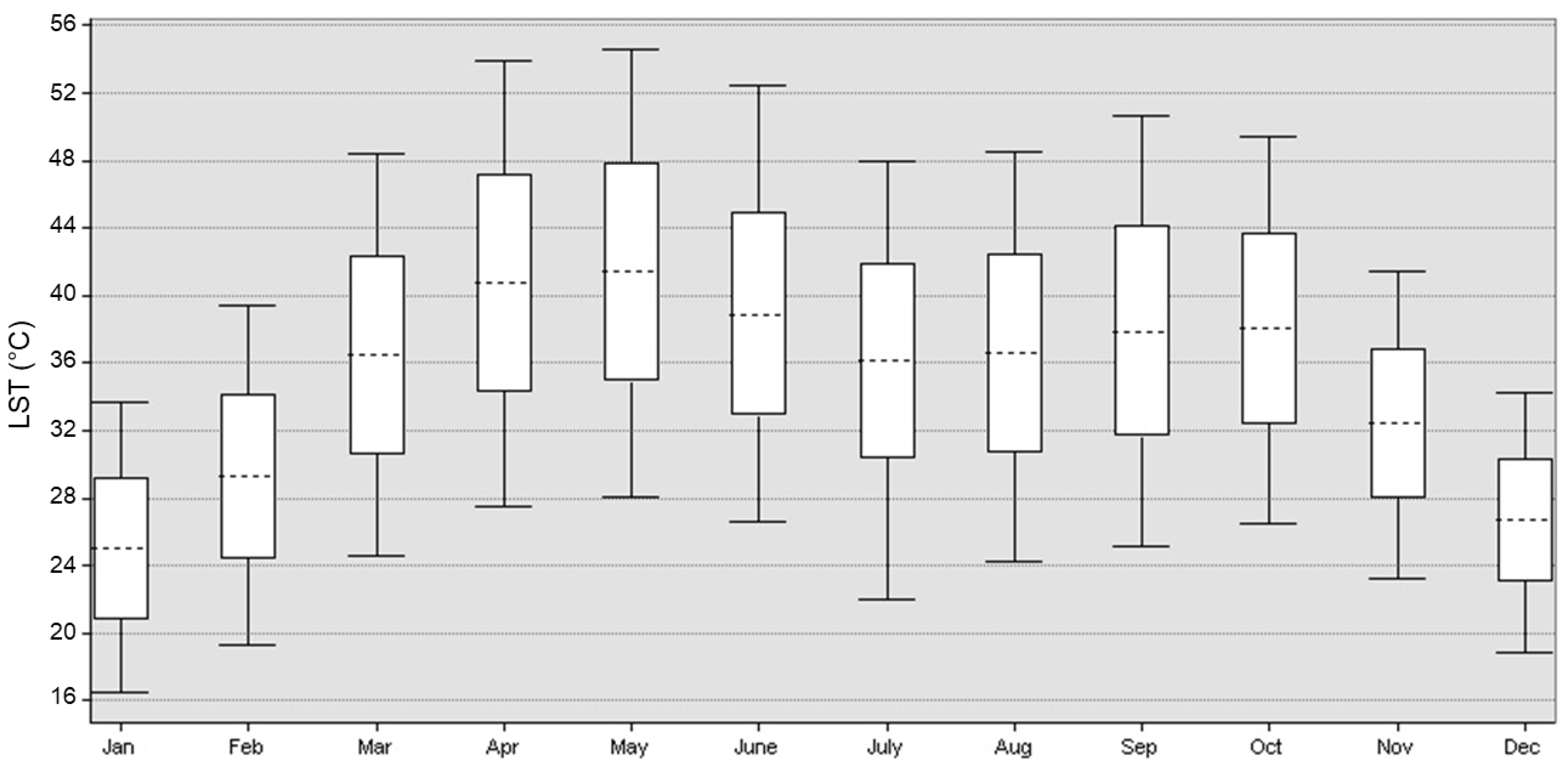
3.2.2. Characterization of Intra-Annual Change

Figure 9 shows the seasonal variability in the LST over the period 2001–2021, and it can be observed that the LST fluctuates throughout the year. The LST has a seasonal peak from April to June, while December and January have the lowest LST mean values. Further, it can be seen from Figure 9 that the LST usually starts to rise in January, reaches its maximum in May, and then decreases until December.

3.2.3. Characterization of Spatial Change

Spatial variations in the long-term mean annual LST for 2001 to 2021 at a 30 m resolution are depicted in Figure 10, and vary from 24 to 47 °C. It can be observed that the western parts have higher temperatures compared to the eastern and southern parts of Rajasthan. The hyper-arid partially irrigated zone and the arid western plains show less variation, while the sub-humid southern plains show the maximum variation over the 21 years. The maximum number of pixels which had a 43–47 °C LST was observed in 2016, followed by 2009 and 2001. Similarly, the maximum area which had a 24–33 °C LST was observed in 2021, followed by 2020.

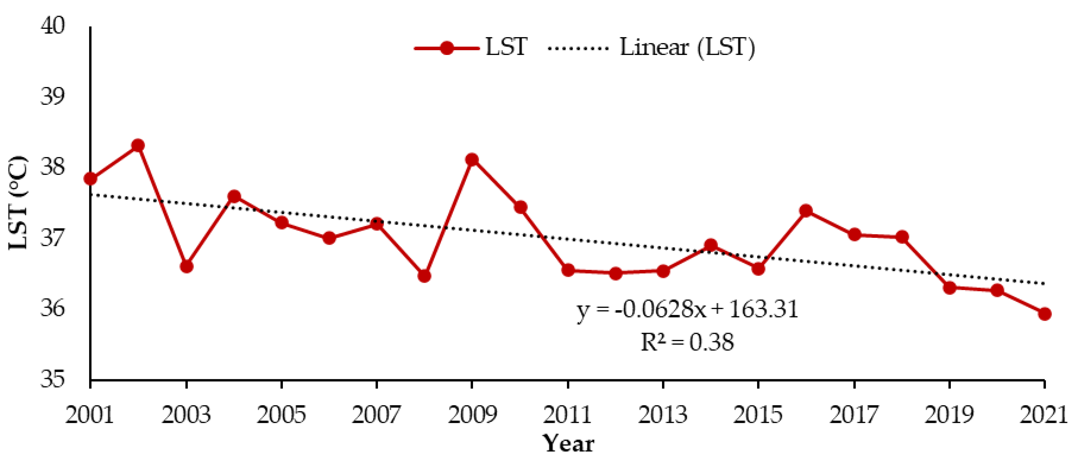
3.2.4. Trend Analysis of LST

Figure 11 depicts the trend in the mean LST across Rajasthan for the 21 years (2001–2021). A linear regression model was developed to detect temporal variations in the LST since 2001 by calculating the average LST for all pixels for the whole of Rajasthan. The results indicate an overall decreasing trend in the LST, with a negative correlation of 0.38 over 2001–2021. The mean LST values vary from ~35.9 to 38.3 °C. In Figure 12A, both increasing and decreasing trends are shown for the mean annual LST data. The magnitude of the change in the LST ranges from −0.26 to 0.30 °C per year. It can be observed that the majority of the pixels (78.65%) have a decreasing trend (S < 0), with the southern and southeastern parts showing the highest declining rates, whereas 21.35% of the pixels have increasing rates, and are concentrated mainly in the western parts of Rajasthan. Figure 12B shows the statistical significance level of the LST trend over the 21 years, and reveals that all of the regions’ trends are insignificant. About 50% of the pixels show significant changes (p < 0.05), and are located mainly in the southern and southeastern parts, whereas the rest of the pixels show a non-significant difference (p > 0.05) in the annual LST.

3.3. Evapotranspiration

3.3.1. Characterization of Annual Change

The annual temporal variations in ET for the 21 years is presented in Figure 13. The maximum fluctuations in the temporal ET pattern are observed to have occurred in 2020, while the minimum was in 2002. The ET values corresponding to 2002 and 2003 appear lower (~350 mm) when compared to the other years considered here. The maximum and minimum ET values occurred in 2020 and 2002, respectively. The median ET varies between ~240 and ~390 mm throughout the period. The 25th and 75th percentile values range from ~120 to ~200 mm and from ~350 to ~590 mm, respectively, from 2001 to 2020.

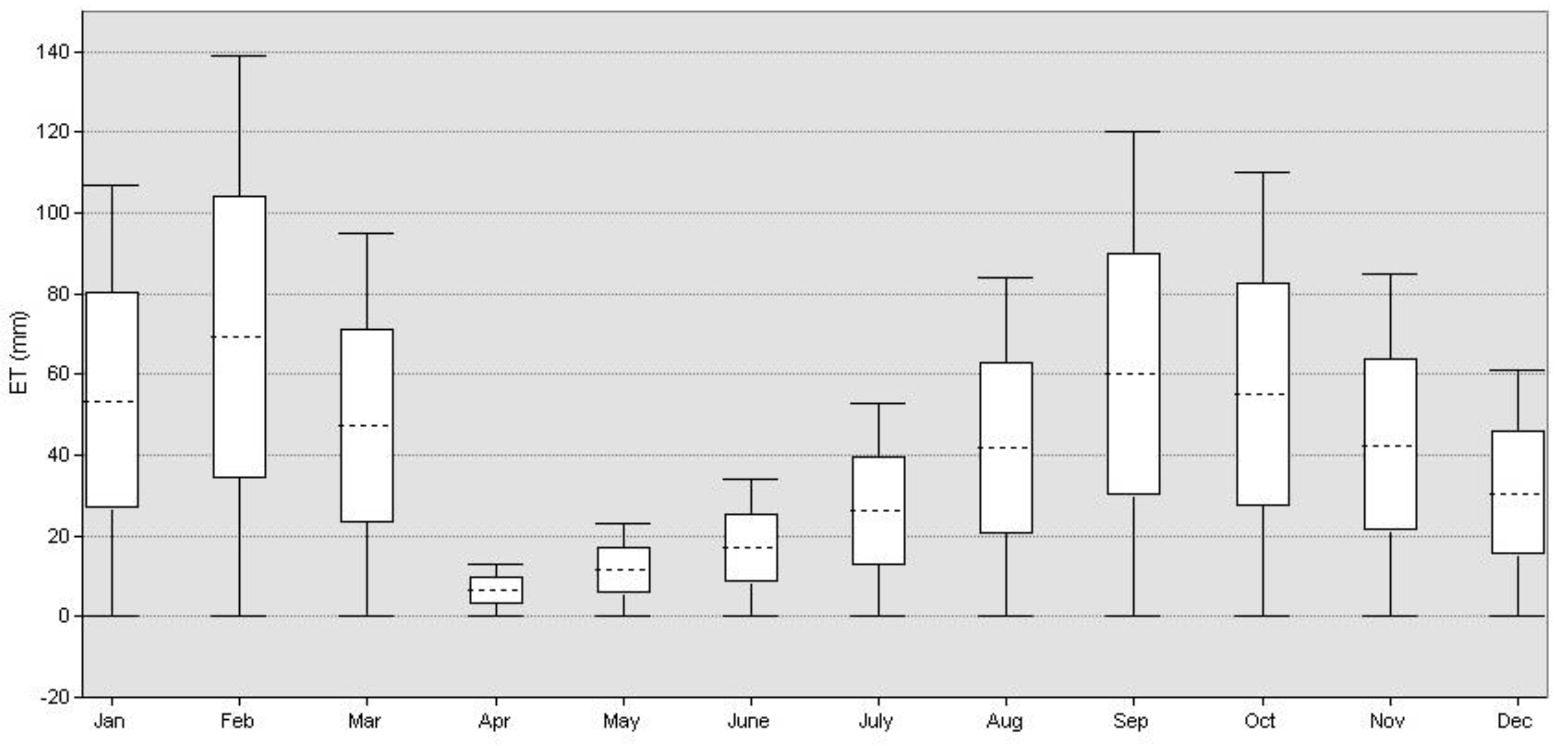
3.3.2. Characterization of Intra-Annual Change

Figure 14 depicts the mean monthly ET for the twenty-one years (2001–2021). Further, we noticed that the monthly ET values fluctuate throughout the year. It can also be observed that ET reaches its seasonal peak in February, while the lowest values for ET occur in April. Additionally, it has been noted that ET often begins to rise in January, peaks in February, and then declines until April, and then, once more, it starts increasing until September, and decreases until December.

3.3.3. Characterization of Spatial Change

Spatial variations in the annual ET from 2001 to 2021 at a 30 m resolution are depicted in Figure 15. The yearly ET varies from 0 to 821 mm. These maps indicate a decreasing trend in ET from the southern and eastern parts to the northern and western parts of Rajasthan. The south and southeastern parts of Rajasthan have a higher ET, which includes the humid southern plains, the sub-humid southern plains, and the humid southeastern plains. The maximum number of pixels with a low ET (0–50 mm) were observed in 2002, followed by 2009. It can also be observed that ET increased in most parts, particularly in the southern and southeastern regions, between 2001 and 2021.

3.3.4. Trend Analysis of ET

Figure 16 depicts the trend in the mean ET for the twenty-one years (2001–2021) for Rajasthan. A linear regression model was created to determine the ET variations since 2001, by averaging the mean ET across all the pixels for the whole state of Rajasthan. With a positive correlation of 0.71 between the ET values over 2001–2021, an overall increasing temporal trend in ET was observed. The mean annual ET values for Rajasthan vary from ~54 to 181 mm.

Figure 17A indicates that most of the area (98.24%) shows a positive trend. Only a few pixels (1.76%) have a negative for the mean annual ET and, by incorporating the significance level from Figure 17B, it is found that 90.21% of the area shows a significant positive change in ET, and only 16.80% of the area shows no trend in ET.

3.4. Normalized Difference Vegetation Index (NDVI)

3.4.1. Characterization of Annual Change

The boxplot corresponding to the annual NDVI temporal patterns indicates that the NDVI varied slightly between 2001 and 2021 (Figure 18). The mean of all the NDVI values from January to December is contained in the NDVI data from 2001 to 2021. The NDVI values were at their highest (~0.74) and lowest (~−0.15) points in 2020 and 2005, respectively. The NDVI experienced its highest variations in 2017 and 2020, while its greatest downward fluctuations were in 2008 and 2010. Additionally, the NDVI’s 75th percentile lies between 0.43 and 0.52, while the 25th percentile of the NDVI did not show any significant variations across the twenty-one years. In addition to this, the NDVI varied between −0.15 and 0.75 from 2001 to 2021.

3.4.2. Characterization of Intra-Annual Change

Figure 19 shows the NDVI seasonal patterns for the entire Rajasthan state. The boxplot displays the mean monthly NDVI values for 2001 to 2021. This study area’s NDVI values are shown to be lowest in June, with seasonal peaks in the NDVI occurring in February and September. Additionally, it can be demonstrated that the monthly NDVI values fluctuate less during the summer than during the monsoon and winter seasons. Further, it has been noted that vegetation greening (NDVI) often begins in May or June, peaks in September, then shows a slight decrease from October to December, and again reaches its maximum value in the month of February, and after that decreases until April or May. This shows the relationship of the NDVI values with the cropping season (Kharif, Rabi, and Zaid).

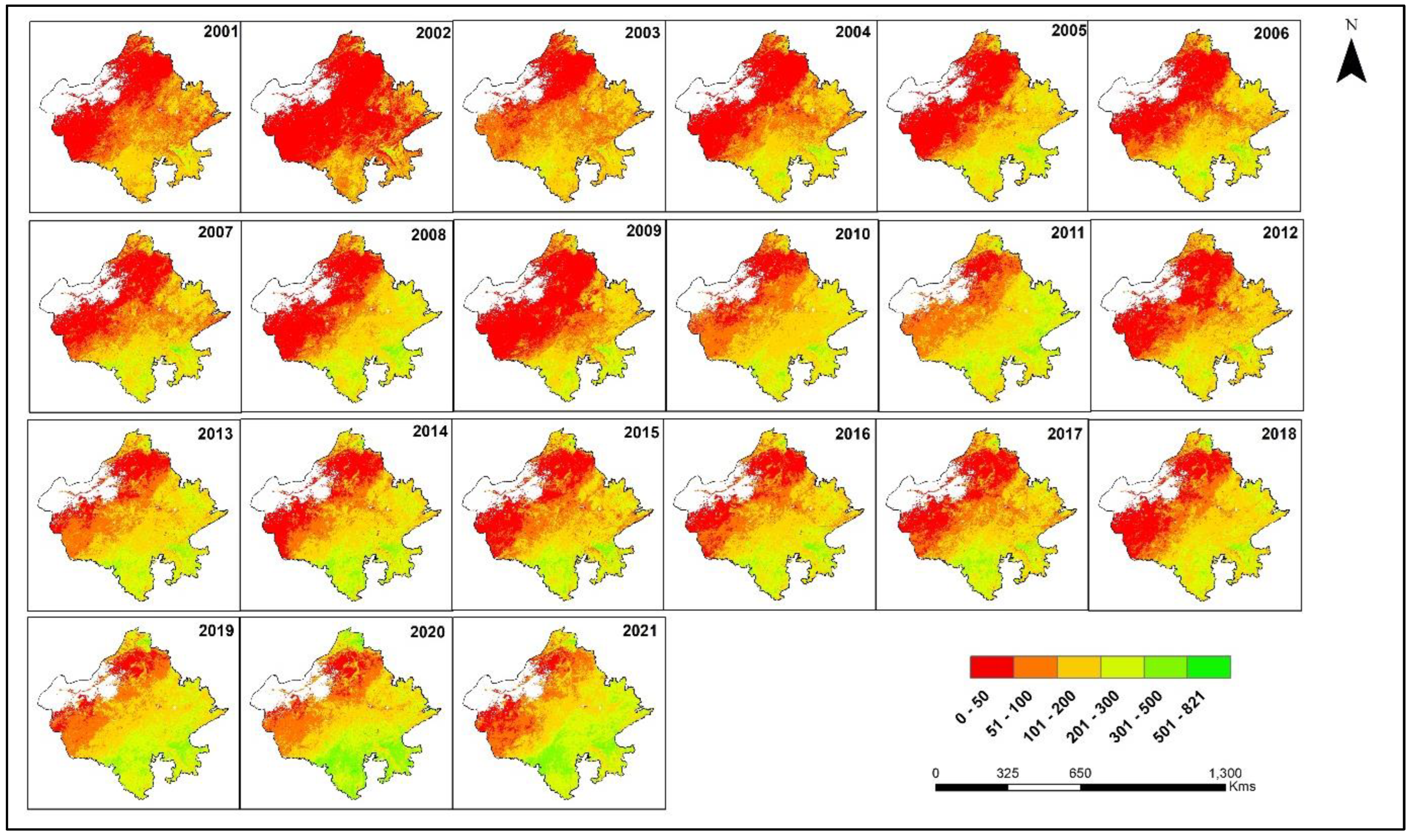
3.4.3. Characterization of Spatial Change

Figure 20 depicts the variations in the mean annual NDVI for 2001–2021 at a 30 m resolution. The NDVI varied from −0.15 to 0.74. The NDVI increased in Rajasthan over time, which reflects the increased greenness in Rajasthan. Among all the years, the maximum number of green pixels was recorded in 2021. In 2001, on the other hand, the trend was the exact opposite, with lower NDVI values covering much of the basin. Despite a solid upward trend in the NDVI, the inter-annual variation has increased since 2009. Most of the areas with high NDVI values fall under the following ACZs: the semi-arid eastern plains, the humid southeastern plain, the humid southern plains, the sub-humid southern plains, and the flood-prone eastern plain. The lowest NDVI values were observed in the following areas of the ACZs: the arid western plain and the hyper-arid partially irrigated zone. Overall, a significantly increasing trend in the NDVI was observed across the study area.

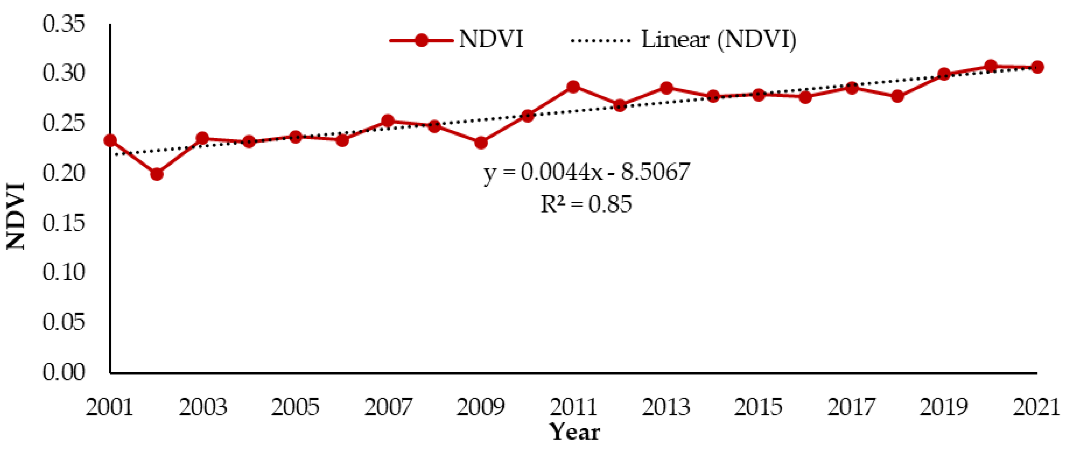
3.4.4. Trend Analysis of NDVI

Figure 21 shows the mean NDVI trend for Rajasthan during 2001–2021. A linear regression model was developed by computing the mean NDVI over all the pixels for the entirety of Rajasthan. With a positive correlation of 0.85 between 2001 and 2021, an overall increasing trend in the NDVI was detected. The mean annual NDVI varied between ~0.20 and 0.31. Sen’s slope values and the MK test for significant trends in the mean annual NDVI at the pixel level are presented in Figure 22A,B. From 2001 to 2021, there were more pixels with improved vegetation than with degraded vegetation. The NDVI increased for 96.5% of the studied area (S > 0), primarily in the south and east, while it dropped for 3.4% of the pixels (S < 0). A statistically significant difference (p < 0.05) was observed for 83.7% of the total pixels. In addition to this, it was also observed that the NDVI significantly increased over the Indira Gandhi Canal command area in the Jaisalmer district of Rajasthan, which is in the hyper-arid and drought-prone regions. The NDVI decreased for some of the pixels in the Jaipur and Jaisalmer districts.

3.5. Correlation between Hydroclimatic Parameters and Vegetative Indices

A pair-wise Pearson correlation coefficient test was implemented to quantify the association between the study parameters. Except for the RF-LST, all the pairs had a significant association between themselves (Figure 23). The highest positive correlation can be observed for ET-NDVI (0.86), followed by ET-RF, whereas the NDVI-LST shows the highest negative correlation (−0.55), followed by ET-LST (−0.46). Overall, we can infer that the LST is negatively correlated with the other parameters, and the other variables are positively correlated.

4. Discussion

4.1. Spatiotemporal Variation in Rainfall

The annual rainfall exhibited a high inter-annual variability during 2001–2021. Strong El Nino conditions were pervasive in 2002, resulting in the lowest rainfall received [33,45,46]. For the 21 years, the median of the annual rainfall is observed to lie in the center of the box, indicating that the annual rainfall follows a normal distribution. The mean monthly variations in precipitation over the last twenty-one years in Rajasthan show that the maximum rainfall is received in July (~640 mm), followed by August (~625 mm) and September (~305 mm), while the lowest mean rainfall is recorded in December. This concurs with previous research conducted in Rajasthan [47,48]. Saini et al. [33] also stated that around two-thirds of the annual rainfall is received in only two months, viz., July and August, while December accounts for only around 0.49% of the yearly rainfall. The spatial variation in the annual rainfall shows decreasing gradients from the southern and southeastern to the western regions of Rajasthan. The western ACZs received the lowest rainfall (8–486 mm), which includes a hyper-arid partially irrigated zone, the arid western plains, the irrigated northwestern plains, and an internal- drainage dry zone. In contrast, more than 1400 mm fell on the transitional plateau of the Luni Basin, and the humid and sub-humid southern plains. A similar result was reported by Meena et al. [47]. The presence of the Aravalli Mountains, which spread from the northeast to southwest in central Rajasthan, is primarily responsible for this decrease in annual average rainfall from east to west [31,49]. Relatively low annual- rainfall variability has been observed in areas of high precipitation. Therefore, the frequent occurrence of drought conditions in the arid and semi-arid regions is attributed to low rainfall and high variability. These findings concur with those of Saini et al. [33], Narain et al. [50], and Kundu and Datta [51].

The MK test and Sen’s slope estimator assessed the spatial distribution of annual rainfall trends and their magnitude from 2001 to 2021. All the pixels with S > 2 mm per year show an increasing trend in annual rainfall. Among all the ACZs, three ACZs, namely the humid southeastern plains, the sub-humid southern plains, and the transitional plains of the Luni Basin, have observed a high positive magnitude (S~31 mm per year). These findings are consistent with earlier studies [33,52,53]. All the pixels in western Rajasthan exhibited increasing trends, but the magnitude was less, and this result is consistent with those of Meena et al. [47], Basistha et al. [54], Kharol et al. [55], Kumar et al. [56], and Singh et al. [57]. This increasing trend is significant mainly in four ACZs: the irrigated northwestern plains, the internal-drainage dry zone, the sub-humid southern plains, and the humid southeastern plains. Similar findings were observed by Meena et al. [47], Sharma et al. [48], and Deoli and Rana [58]. To comprehend these trends, it seems most likely that rising sea surface temperatures and surface latent heat flow across the tropical Indian Ocean [59,60] are accountable. The increasing rainfall intensity may also be primarily influenced by the increasing atmospheric moisture content [61]. The western arid region, which is assumed to be the most drought-prone area, has observed an increase in its mean annual rainfall, which could be highly beneficial for agricultural and groundwater recharge. Meena et al. [47] and Poonia and Rao [62] also reported an increasing trend in rainfall in the arid climate of Rajasthan. Saini et al. [33] studied rainfall variability and trends for 1961–2017, and found a significant increasing trend in the arid and semi-arid regions.

4.2. Spatiotemporal Variation in Land Surface Temperature

The LST is an essential indicator of the Earth’s surface energy balance [63]. Remote sensing-based LST data are used to explore the consequences of vegetative greenness and LULC change [10,64]. The annual LST temporal patterns show that the LST fluctuated slightly between 2001 and 2021. These fluctuations might be due to the heterogeneity of vegetation coverage and rainfall patterns [65]. In addition to these factors, some natural factors, such as parent material, soil condition, surface roughness, and albedo, are some important factors influencing the LST [66]. The monthly evaluation revealed that April, May, and June had regions with higher LST values, whereas December and January showed lower LST values. Due to the variations in the angle of inclination of the Earth with the Sun throughout the year, there is significant variation in the Incoming solar radiation at different locations [67]. The LST showed a decreasing trend during the monsoon season (June to August), which may be because, in the monsoon season, most of the land is occupied with dense crops or vegetation, which reduces the LST; however, in summer, the vegetation cover over the land is at a minimum, resulting in high LSTs [63]. Several studies have shown a relationship between lower vegetation greenness or NDVI values with higher LST values [65]. So, the LST decreased during the peak vegetative growth of the Rabi and Kharif crops.

It was observed that the western parts have higher temperatures as compared to the eastern and southern parts of Rajasthan. Different climatic and landscape components, such as rainfall, solar insolation, air temperature, elevation, sparse vegetation, and soil properties, significantly impact heat emission and absorption, affecting the LST variations [68]. The annual rainfall also decreases from east to west, creating moisture fluxes in arid and semi-arid regions [55]. This is primarily due to the Aravalli mountains, which extend from central Rajasthan’s northeast to southwest [49]. The western part of Rajasthan has unsuitable soil conditions and texture, low vegetation cover, and arid climatic conditions [66]. Therefore, this zone has a higher LST than the eastern and southern parts. The LST is significantly impacted by the study area’s elevation, which varies from −6 to 1698 m. The temperature falls with increasing elevation, which is evident from many studies, and the same was observed in this study [69].

To analyze the annual trend of the LST over the 21 years (2001–2021), a linear regression model shows a decrease in the LST by 6.2 °C for the entirety of Rajasthan. It was observed that the LST increased in 2002 and 2009, which may be attributed to the prevalence of drought or low rainfall and low vegetation cover [33,70]. The MK test and Sen’s slope were used to determine the spatial pattern of annual rainfall trends at the pixel level in 2001 and 2021. A decreasing trend (S < 0) was observed in the southern and southeastern regions as rainfall increased, a significant factor for high vegetative greenness. There is a general declining trend in the LST as vegetation becomes denser (exhibited by the higher value of the NDVI). The dense vegetation canopy provides an efficient barrier against incoming solar radiation and enhances the evaporative cooling effect, which has a moderating effect on an increasing surface temperature. Thus, the land surface temperature decreases with increasing vegetation cover. Furthermore, a noticeable decreasing trend was found over the Indira Gandhi Canal, which could be due to the area under irrigation increasing over time, as a result of the expanding canal system [71]. As in other tropical regions [72,73,74], our results also indicate that eastern Rajasthan is experiencing a colder shift yearly.

4.3. Spatiotemporal Variation in Evapotranspiration

The spatiotemporal pattern of the mean annual ET clearly indicates strong variations corresponding to native vegetation types and prevailing climatic conditions. The annual pattern of ET exhibits an increasing trend. This can be attributed to the fact that rainfall has increased during the last 21 years and is a prime factor for high vegetation greenness. Several studies have also reported that changes in ET are most likely caused by changes in climatic parameters (rainfall and LST), rather than changes in the NDVI and EVI [73,75]. All the parameters, including the median, the 25th, and the 75th percentile, were at a minimum during 2002 because it was a drought year in Rajasthan [33,70]. The seasonal variation in ET clearly shows peaks and valleys based on the crop season. The ET rate was high during the peak vegetative stage of the Rabi and Kharif seasons, while it was low during the summer due to less vegetation coverage. The low ET levels during the summer were accompanied by the senescence of deciduous forests and crops, low relative humidity, very high temperatures, and low soil moisture [76]. The low ET rate in the winter may be due to low mean temperature and more diffuse solar insolation [77,78]. The results of this study are highly consistent with the output of Poonia and Rao (2013) [62]. The annual ET varied between 0 and 821 mm for the entire state of Rajasthan (2001–2021). Rajasthan’s arid regions, with deserts and sparsely vegetated areas in the western parts, had the lowest ET (50 mm), while the southern part of the state had the highest ET (>500 mm). In the western region, low rainfall, very little or no available soil moisture, and poor vegetation are the reasons for the low ET rate. Our results are consistent with those of Goroshi et al. [76]. The mean annual ET of the state was 126 mm, with maximum and minimum values of 54.3 mm and 181.3 mm in 2002 and 2021, respectively. The ET rate decreased in 2002 due to the drought phenomenon [70]. Researchers from various climatic and geographical regions have performed this sort of analysis. Matzneller et al. [79] analyzed the annual ET trends over Bologna–Cadriano, Italy, from 1952 to 2007, using the Hargreaves and Samani Method, and suggested that rising air temperatures are accountable for the changes. Specifically, in the western arid and semi-arid regions, the enormous increase in the amount of land irrigated by canals, and a modification in cropping patterns and cultivars, may have enhanced the annual ET [71,80].

The estimation of the ET trend from the MK test and Sen’s slope estimator revealed that most of the area (98.24%) showed a positive trend (S > 0), while 1.76% of the pixels had a negative trend (S < 0). This significant increasing (p < 0.05, S > 0) trend was mainly concentrated in the southern, southeastern, and northern regions, and was highly dependent on native vegetation, soil properties, and climatic conditions. In addition to this, a significant increasing (p < 0.05, S > 0) trend was observed for the canal area, and this is mainly attributed to a proportionate increase in crop area as a result of the increasing canal networks [71]. Figure 24 depicts a part of the Indira Gandhi Canal (IGC) in the western dry lands that has entirely changed over time. Before human interference, this area was covered sandy barren land, but greenness spread with the distinctively visible expansion of agricultural fields as time passed. There is a decreasing trend for ET, particularly in the Jaipur district, which is experiencing vegetative degradation due to urbanization and industrialization over the years [63,81]. Extensive industrialization has caused substantial cropland losses [82,83] and regional climate change [84,85]. Google Earth images also confirm that the built-up areas and industries have expanded over the years (Figure 25 and Figure 26).

4.4. Spatiotemporal Variation in NDVI

The annual temporal pattern of the NDVI shows that it fluctuated slightly between 2001 and 2021. Rajasthan’s uneven rainfall distribution caused this variation in vegetation greenness. Several researchers have revealed that temporal variations in the NDVI are closely related to precipitation [10,86,87,88]. However, a one- or two-month lag exists between the NDVI and rainfall [10,89].

The spatial variability in the mean annual NDVI ranged from −0.15 to 0.74 during 2001 to 2021. This spatial variability has arisen primarily due to the uneven rainfall distribution in the state [31]. The ACZ regions encompassing the humid southern plains, the humid southeastern plain, the flood-prone eastern plain, and the sub-humid southern plains have a high NDVI as a result of sufficient precipitation, ranging from 800 to 1000 mm, which helps to increase the cultivation of Kharif crops and the residual moisture helps to grow crops in the Rabi season also. The central part of Rajasthan state, denoted by the internal-drainage dry zone, the transitional plain of the Luni Basin, and the semi-arid eastern plains, had a medium NDVI. This could be explained by the medium rainfall and high LST, along with the seasonal fallow situation of the agricultural lands. The western part of Rajasthan had NDVI values of less than 0.15. The sandy Thar Desert, located in the western part of Rajasthan, has a typical arid climate with very little rainfall and intense heat waves, making it difficult for vegetation to grow there, other than Caryophyllales (cactus) plants [14,90]. However, recent irrigation management strategies have resulted in some changes in these areas [14]. Crops are currently grown widely in the heart of the desert. As a result, a spatial shift in the spread of greenness has become evident over time. However, vegetation conditions were substantially stressed in 2002. Several researchers have also reported that a severe drought prevailed during Kharif in 2002 [31,91]. Despite the predominance of drought conditions in Rajasthan in 2002, the eastern parts of the state remained unharmed. Furthermore, the topography of Rajasthan exhibits significant variations, with an elevation range of −6 to 1698 m above sea level. These topographical conditions have a significant influence on the patterns of vegetation distribution across Rajasthan.

Regarding this temporal trend, the NDVI values increased from 2001 to 2021, with a positive correlation of 0.85. However, the NDVI values in 2002 were far less than those of 2001 and 2003, indicating the stressed vegetation during the monsoon due to drought. It is more interesting that the NDVI showed an increasing trend around the Indira Gandhi Canal. This might be due to the enhancement of irrigation facilities due to the Indira Gandhi Canal, the restoration of degraded land, cropping-pattern changes, sufficient rainfall, the cultivation of wastelands, and rainwater-harvesting structures, while proper policy interventions might be the reasons in other parts of the study area [71]. The Indira Gandhi Nahar Pariyojana (IGNP) stretches over seven districts in Rajasthan: Churu, Barmer, Sriganganagar, Hanumangarh, Bikaner, Jodhpur, and Jaisalmer, and has brought about tremendous changes over time [14]. After 2012, the canal’s impact was felt widely over the western drylands, resulting in a substantial surge in agricultural productivity due to improved irrigation facilities. Sur and Chauhan (2019) [71] also reported a significant change (1–78%) in the net primary productivity (NPP) during 1982–2012 across the IGC area. Figure 24 illustrates an area of the IGNP canal located in the western drylands, which has undergone significant transformations over a period of time. Some of the pixels exhibit a noticeable decrease in the NDVI, particularly within the Jaipur district. This decline may be attributed to factors such as industrialization, urbanization, groundwater depletion, inadequate irrigation practices, and alterations in cropping patterns. According to Dangayach et al. [92], there has been a significant decrease in agricultural land, which reduced from 47.20% to 25.50%, while the built-up land recorded a rise from 22.80% to 44.2% during the period of the past two decades (2000–2020). Urbanization and industrialization have led to significant reductions in cropland [82,83], and have also contributed to regional climate change [84,85]. Google Earth images (Figure 25 and Figure 26) have also confirmed that the built-up areas and industries have expanded over the years.

4.5. Correlation between Hydroclimatic Parameters and Vegetative Index

Temperature and rainfall are widely recognized as the primary factors which characterize the climate of a region and exert significant effects on vegetation [93]. ET-NDVI has a significant positive correlation (0.86), while ET-RF shows a slightly lower positive correlation (0.40). On the contrary, the NDVI-LST has the highest negative correlation (−0.55), followed by ET-LST, with a negative correlation of −0.46. These findings reveal a significant relationship between the NDVI and climatic factors, and vegetation growth is affected by precipitation, the LST, and ET. The NDVI value increases with an increase in precipitation [94]. Generally, high LST values are usually associated with low NDVI areas, and vice versa. The areas with high LST values are characterized by the presence of built-up areas and exposed bare-ground surfaces. In contrast, the low LST zones are primarily associated with the presence of water bodies and extensive vegetation cover. The presence of a dense vegetation canopy serves as an effective shield against incoming solar radiation, hence, enhancing the evaporative cooling process of the vegetation and reducing the surface temperature. In general, a negative NDVI is indicative of the existence of water bodies or wetlands. Therefore, it may be concluded that the LST–NDVI relationship for water bodies or wetlands is not consistent. This result is highly consistent with that of Abera et al. [95], Guha and Govil [96], and Garai et al. [97]. Furthermore, it has been observed that there is a negative relationship between rainfall and LST, indicating that the LST is influenced by variations in rainfall. The combination of low rainfall and a higher LST value suggests that the vegetation has a low moisture content, which could be one of the factors contributing to forest fires [98]. Overall, these findings show a relationship between the NDVI, rainfall, and LST.

Assessing climate change and its influence on vegetation dynamics using high-resolution satellite data is the first step in providing valuable information for researchers, planners, and agricultural decision makers to mitigate climate change’s impact, restore degraded lands, and achieve sustainable development goals by establishing land exploration and restoration policies. We advocate for the authorities to draw particular attention to achieving land degradation neutrality in the study area, as a significant portion of Rajasthan is affected by desertification disasters. This study employed high-resolution remote sensing products to analyze the vegetation dynamics of Rajasthan. However, it is important to note that there is a degree of uncertainty associated with these products, due to possible product quality issues. The present study, however, primarily concentrated on performing an initial analysis of vegetation change. Nonetheless, it is important to conduct more investigations in order to fully investigate the underlying mechanisms responsible for the observed inconsistencies. There is a need to quantify the relative contributions climate change and human activities have made to vegetation changes using geospatial modeling.

5. Conclusions

Vegetation monitoring is difficult in Rajasthan due to the intricate topography and extreme climatic variability. Thus, a remote sensing technique is a boon for analyzing and monitoring vegetation trends, and evaluating its response to a changing climate. This study explored the long-term (21 years) spatiotemporal variability in vegetation greenness using the NDVI and its relationship with three hydroclimatic factors, viz., rainfall, LST, and ET, which were derived from satellite images of Rajasthan. The results show a significant change in all five parameters during the study period from 2001 to 2021. This study’s results provide direct evidence of a considerable decrease in degraded lands in Rajasthan, especially in the Indira Gandhi Canal command area, and a simultaneous increase in cropping area. The climatic impact of the increasing or decreasing vegetation trend across Rajasthan is confirmed by the strong correlation between the NDVI and the associated hydroclimatic factors. This study also reveals the efficiency of high-resolution satellite images for monitoring vegetation greenness on a regional level. This study’s outcomes can help to restore degraded lands, achieve ecosystem conservation, and achieve sustainable development goals.

References

1. Kundu, A.; Denis, D.M.; Patel, N.R.; Dutta, D. Long-Term Trend of Vegetation in Bundelkhand Region (India): An Assessment Through SPOT-VGT NDVI Datasets. In Climate Change, Extreme Events and Disaster Risk Reduction; Springer: Cham, Switzerland, 2018; pp. 89–99. [Google Scholar]
2. Liu, Y.; Lei, H. Responses of natural vegetation dynamics to climate drivers in China from 1982 to 2011. Remote Sens. 2015, 7, 10243–10268. [Google Scholar] [CrossRef]
3. Huang, F.; Xu, S. Spatio-temporal variations of rain-use efficiency in the west of Songliao Plain, China. Sustainability 2016, 8, 308. [Google Scholar] [CrossRef]
4. Srivastava, A.; Rodriguez, J.F.; Saco, P.M.; Kumari, N.; Yetemen, O. Global Analysis of Atmospheric Transmissivity Using Cloud Cover, Aridity and Flux Network Datasets. Remote Sens. 2021, 13, 1716. [Google Scholar] [CrossRef]
5. Hou, W.; Gao, J.; Wu, S.; Dai, E. Interannual variations in growing-season NDVI and its correlation with climate variables in the southwestern karst region of China. Remote Sens. 2015, 7, 11105–11124. [Google Scholar] [CrossRef]
6. Wu, C.; Venevsky, S.; Sitch, S.; Yang, Y.; Wang, M.; Wang, L.; Gao, Y. Present-day and future contribution of climate and fires to vegetation composition in the boreal forest of China. Ecosphere 2017, 8, e01917. [Google Scholar] [CrossRef]
7. Scheffer, M.; Holmgren, M.; Brovkin, V.; Claussen, M. Synergy between small-and large-scale feedbacks of vegetation on the water cycle. Glob. Change Biol. 2005, 11, 1003–1012. [Google Scholar] [CrossRef]
8. Quillet, A.; Peng, C.; Garneau, M. Toward dynamic global vegetation models for simulating vegetation–climate interactions and feedbacks: Recent developments, limitations, and future challenges. Environ. Rev. 2010, 18, 333–353. [Google Scholar] [CrossRef]
9. Hamid, M.; Khuroo, A.A.; Malik, A.H.; Ahmad, R.; Singh, C.P.; Dolezal, J.; Haq, S.M. Early evidence of shifts in alpine summit vegetation: A case study from Kashmir Himalaya. Front. Plant Sci. 2020, 11, 421. [Google Scholar] [CrossRef]
10. Kumari, N.; Srivastava, A.; Dumka, U.C. A long-term spatiotemporal analysis of vegetation greenness over the himalayan region using google earth engine. Climate 2021, 9, 109. [Google Scholar] [CrossRef]
11. Kumar, K.C.A.; Reddy, G.P.O.; Masilamani, P.; Sandeep, P.; Turkar, S.Y. Integrated drought monitoring index: A tool to monitor agricultural drought by using time series space-based earth observation satellite datasets. Adv. Space Res. 2021, 67, 298–315. [Google Scholar] [CrossRef]
12. Singh, R.N.; Sah, S.; Chaturvedi, G.; Das, B.; Pathak, H. Innovative trend analysis of rainfall in relation to soybean productivity over western Maharashtra. J. Agrometeorol. 2021, 23, 228–235. [Google Scholar] [CrossRef]
13. Singh, R.N.; Sah, S.; Das, B.; Chaturvedi, G.; Kumar, M.; Rane, J.; Pathak, H. Long-term spatiotemporal trends of temperature associated with sugarcane in west India. Arab. J. Geosci. 2021, 14, 1955. [Google Scholar] [CrossRef]
14. Sur, K.; Dave, R.; Chauhan, P. Spatio-temporal changes in NDVI and rainfall over Western Rajasthan and Gujarat region of India. J. Agrometeorol. 2018, 20, 189–195. [Google Scholar]
15. Mariano, D.A.; dos Santos, C.A.; Wardlow, B.D.; Anderson, M.C.; Schiltmeyer, A.V.; Tadesse, T.; Svoboda, M.D. Use of remote sensing indicators to assess effects of drought and human-induced land degradation on ecosystem health in Northeastern Brazil. Remote Sens. Environ. 2018, 213, 129–143. [Google Scholar] [CrossRef]
16. Guo, E.; Wang, Y.; Wang, C.; Sun, Z.; Bao, Y.; Mandula, N.; Jirigala, B.; Bao, Y.; Li, H. NDVI indicates long-term dynamics of vegetation and its driving forces from climatic and anthropogenic factors in Mongolian Plateau. Remote Sens. 2021, 13, 688. [Google Scholar] [CrossRef]
17. Rihan, W.; Zhang, H.; Zhao, J.; Shan, Y.; Guo, X.; Ying, H.; Deng, G.; Li, H. Promote the advance of the start of the growing season from combined effects of climate change and wildfire. Ecol. Indicat. 2021, 125, 107483. [Google Scholar] [CrossRef]
18. Zeng, Z.; Wu, W.; Ge, Q.; Li, Z.; Wang, X.; Zhou, Y.; Zhang, Z.; Li, Y.; Huang, H.; Liu, G.; et al. Legacy effects of spring phenology on vegetation growth under preseason meteorological drought in the Northern Hemisphere. Agric. For. Meteorol. 2021, 310, 108630. [Google Scholar] [CrossRef]
19. Bai, Y.; Li, S.; Liu, M.; Guo, Q. Assessment of vegetation change on the Mongolian Plateau over three decades using different remote sensing products. J. Environ. Manag. 2022, 317, 115509. [Google Scholar] [CrossRef]
20. Nemani, R.R.; Keeling, C.D.; Hashimoto, H.; Jolly, W.M.; Piper, S.C.; Tucker, C.J.; Myneni, R.B.; Running, S.W. Climate-driven increases in global terrestrial net primary production from 1982 to 1999. Science 2003, 300, 1560–1563. [Google Scholar] [CrossRef]
21. Zhu, Z. Change detection using landsat time series: A review of frequencies, preprocessing, algorithms, and applications. ISPRS J. Photogramm. Remote Sens. 2017, 130, 370–384. [Google Scholar] [CrossRef]
22. Srivastava, A.; Sahoo, B.; Raghuwanshi, N.S.; Singh, R. Evaluation of variable-infiltration capacity model and MODIS-terra satellite-derived grid-scale evapotranspiration estimates in a River Basin with Tropical Monsoon-Type climatology. J. Irrig. Drain. Eng. 2017, 143, 04017028. [Google Scholar] [CrossRef]
23. Piao, S.; Wang, X.; Park, T.; Chen, C.; Lian, X.U.; He, Y.; Bjerke, J.W.; Chen, A.; Ciais, P.; Tømmervik, H.; et al. Characteristics, drivers and feedbacks of global greening. Nat. Rev. Earth Environ. 2020, 1, 14–27. [Google Scholar] [CrossRef]
24. Venter, Z.S.; Scott, S.L.; Desmet, P.G.; Hoffman, M.T. Application of Landsat-derived vegetation trends over South Africa: Potential for monitoring land degradation and restoration. Ecol. Indic. 2020, 113, 106206. [Google Scholar] [CrossRef]
25. Huete, A. Vegetation’s responses to climate variability. Nature 2016, 531, 181–182. [Google Scholar] [CrossRef]
26. Yang, J.; Gong, P.; Fu, R.; Zhang, M.; Chen, J.; Liang, S.; Xu, B.; Shi, J.; Dickinson, R. The role of satellite remote sensing in climate change studies. Nat. Clim. Change 2013, 3, 875–883. [Google Scholar] [CrossRef]
27. Wardlow, B.D.; Egbert, S.L. A comparison of MODIS 250-m EVI and NDVI data for crop mapping: A case study for southwest Kansas. Int. J. Remote Sens. 2010, 31, 805–830. [Google Scholar] [CrossRef]
28. Hereher, M.E. The status of Egypt’s agricultural lands using MODIS Aqua data. Egypt. J. Remote Sens. Space Sci. 2013, 16, 83–89. [Google Scholar]
29. Garroutte, E.L.; Hansen, A.J.; Lawrence, R.L. Using NDVI and EVI to map spatiotemporal variation in the biomass and quality of forage for migratory elk in the Greater Yellowstone Ecosystem. Remote Sens. 2016, 8, 404. [Google Scholar] [CrossRef]
30. Reddy, G.P.O.; Kumar, N.; Sahu, N.; Srivastava, R.; Singh, S.K.; Naidu, L.G.K.; Chary, G.R.; Biradar, C.M.; Gumma, M.K.; Reddy, B.S.; et al. Assessment of spatio-temporal vegetation dynamics in tropical arid ecosystem of India using MODIS time-series vegetation indices. Arab. J. Geosci. 2020, 13, 704. [Google Scholar] [CrossRef]
31. Dutta, D.; Kundu, A.; Patel, N.R.; Saha, S.K.; Siddiqui, A.R. Assessment of agricultural drought in Rajasthan (India) using remote sensing derived Vegetation Condition Index (VCI) and Standardized Precipitation Index (SPI). Egypt. J. Remote Sens. Space Sci. 2015, 18, 53–63. [Google Scholar] [CrossRef]
32. Matsushita, B.; Yang, W.; Chen, J.; Onda, Y.; Qiu, G. Sensitivity of the enhanced vegetation index (EVI) and normalized difference vegetation index (NDVI) to topographic effects: A case study in high-density cypress forest. Sensors 2007, 7, 2636–2651. [Google Scholar] [CrossRef]
33. Saini, D.; Bhardwaj, P.; Singh, O. Recent rainfall variability over Rajasthan, India. Theor. Appl. Climatol. 2021, 148, 363–381. [Google Scholar] [CrossRef]
34. Chen, J.; Jönsson, P.; Tamura, M.; Gu, Z.; Matsushita, B.; Eklundh, L. A simple method for reconstructing a high-quality NDVI time-series data set based on the Savitzky–Golay filter. Remote Sens. Environ. 2004, 91, 332–344. [Google Scholar] [CrossRef]
35. Yadav, B.; Malav, L.C.; Jiménez-Ballesta, R.; Kumawat, C.; Patra, A.; Patel, A.; Jangir, A.; Nogiya, M.; Meena, R.L.; Moharana, P.C.; et al. Modeling and assessment of land degradation vulnerability in arid ecosystem of Rajasthan using analytical hierarchy process and geospatial techniques. Land 2023, 12, 106. [Google Scholar] [CrossRef]
36. Wan, Z. Collection-6 MODIS Land Surface Temperature Products Users’ Guide. 2013. Available online: https://lpdaac.usgs.gov/documents/118/MOD11_User_Guide_V6.pdf (accessed on 29 July 2023).
37. Malav, L.C.; Yadav, B.; Tailor, B.L.; Pattanayak, S.; Singh, S.V.; Kumar, N.; Reddy, G.P.; Mina, B.L.; Dwivedi, B.S.; Jha, P.K. Mapping of land degradation vulnerability in the semi-arid watershed of Rajasthan, India. Sustainability 2022, 14, 10198. [Google Scholar] [CrossRef]
38. Srivastava, A.; Sahoo, B.; Raghuwanshi, N.S.; Chatterjee, C. Modelling the dynamics of evapotranspiration using Variable Infiltration Capacity model and regionally calibrated Hargreaves approach. Irrig. Sci. 2018, 36, 289–300. [Google Scholar] [CrossRef]
39. Mann, H.B. Nonparametric Tests against Trend. Econometrica 1945, 13, 245–259. [Google Scholar] [CrossRef]
40. Kendall, M.G. Rank Correlation Methods, 4th ed.; Charles Grifin: London, UK, 1975. [Google Scholar]
41. Hamed, K.H.; Rao, A.R. A Modified Mann-Kendall Trend Test for Autocorrelated Data. J. Hydrol. 1998, 204, 182–196. [Google Scholar] [CrossRef]
42. Hansen, B.E. Challenges for econometric model selection. Econom. Theory 2005, 21, 60–68. [Google Scholar] [CrossRef]
43. Sen, P.K. Estimates of the Regression Coefficient Based on Kendall’s Tau. J. Am. Stat. Assoc. 1968, 63, 1379–1389. [Google Scholar] [CrossRef]
44. Theil, H. A Rank-Invariant Method of Linear and Polynomial Regression Analysis, Part I; Confidence Regions for the Parameters of Polynomial Regression Equations. Proc. R. Neth. Acad. Sci. 1950, 53, 386–392. [Google Scholar]
45. Mahala, B.K.; Nayak, B.K.; Mohanty, P.K. Impacts of ENSO and IOD on tropical cyclone activity in the Bay of Bengal. Nat. Hazards 2015, 75, 1105–1125. [Google Scholar] [CrossRef]
46. Bhardwaj, P.; Pattanaik, D.R.; Singh, O. Tropical cyclone activity over Bay of Bengal in relation to El Niño-Southern Oscillation. Int. J. Climatol. 2019, 39, 5452–5469. [Google Scholar] [CrossRef]
47. Meena, H.M.; Machiwal, D.; Santra, P.; Moharana, P.C.; Singh, D.V. Trends and homogeneity of monthly, seasonal, and annual rainfall over arid region of Rajasthan, India. Theor. Appl. Climatol. 2019, 136, 795–811. [Google Scholar] [CrossRef]
48. Sharma, S.K.; Sharma, D.P.; Sharma, M.K.; Gaur, K.; Manohar, P. Trend Analysis of Temperature and Rainfall of Rajasthan, India. J. Probab. Stat. 2021, 2021, 6296709. [Google Scholar] [CrossRef]
49. Yadav, R.K.; Rupa Kumar, K.; Rajeevan, M. Characteristic features of winter precipitation and its variability over north-west India. J. Earth Syst. Sci. 2012, 121, 611–623. [Google Scholar] [CrossRef]
50. Narain, P.; Rathore, L.S.; Singh, R.S.; Rao, A.S. Drought Assessment and Management in Arid Rajasthan; Central Arid Zone Research Institute; Jodhpur and NCMRWF: Noida, India, 2006; p. 64. [Google Scholar]
51. Kundu, A.; Dutta, D. Monitoring desertification risk through climate change and human interference using remote sensing and GIS techniques. Int. J. Geomat. Geosci. 2011, 2, 21. [Google Scholar]
52. Pant, G.B.; Hingane, L.S. Climatic changes in and around the Rajasthan desert during the 20th century. J. Climatol. 1988, 8, 391–401. [Google Scholar] [CrossRef]
53. Singh, R.S.; Narain, P.; Sharma, K.D. Climate changes in Luni river basin of arid western Rajasthan (India). Vayu Mandal 2001, 31, 103–106. [Google Scholar]
54. Basistha, A.; Goel, N.K.; Arya, D.S.; Gangwar, S.K. Spatial pattern of trends in Indian sub-divisional rainfall. Jalvigyan Sameeksha 2007, 22, 47–57. [Google Scholar]
55. Kharol, S.K.; Kaskaoutis, D.G.; Badarinath, K.V.S.; Sharma, A.R.; Singh, R.P. Influence of land use/land cover (LULC) changes on atmospheric dynamics over the arid region of Rajasthan state, India. J. Arid Environ. 2013, 88, 90–101. [Google Scholar] [CrossRef]
56. Kumar, V.; Jain, S.K.; Singh, Y. Analysis of long-term rainfall trends in India. Hydrolog. Sci. J. 2010, 55, 484–496. [Google Scholar] [CrossRef]
57. Singh, R.N.; Sah, S.; Das, B.; Potekar, S.; Chaudhary, A.; Pathak, H. Innovative trend analysis of spatio-temporal variations of rainfall in India during 1901–2019. Theor. Appl. Climatol. 2021, 145, 821–838. [Google Scholar] [CrossRef]
58. Deoli, V.; Rana, S. Seasonal trend analysis in rainfall and temperature for Udaipur district of Rajasthan. Curr. World Environ. 2017, 14, 312. [Google Scholar] [CrossRef]
59. Goswami, B.N.; Venugopal, V.; Sengupta, D.; Madhusoodanan, M.S.; Xavier, P.K. Increasing trend of extreme rain events over India in a warming environment. Science 2006, 314, 1442–1445. [Google Scholar] [CrossRef] [PubMed]
60. Rajeevan, M.; Bhate, J.; Jaswal, A.K. Analysis of variability and trends of extreme rainfall events over India using 104 years of gridded daily rainfall data. Geophys. Res. Lett. 2008, 35, 1–6. [Google Scholar]
61. Lacombe, G.; McCartney, M. Uncovering consistencies in Indian rainfall trends observed over the last half century. Clim. Change 2014, 123, 287–299. [Google Scholar] [CrossRef]
62. Poonia, S.; Rao, A.S. Climate change and its impact on Thar desert ecosystem. J. Agric. Phy. 2013, 13, 71–79. [Google Scholar]
63. Khandelwal, S.; Goyal, R.; Kaul, N.; Mathew, A. Assessment of land surface temperature variation due to change in elevation of area surrounding Jaipur, India. Egypt. J. Remote Sens. Space Sci. 2018, 21, 87–94. [Google Scholar]
64. Dos Santos, C.A.; Mariano, D.A.; Francisco das Chagas, A.; Dantas, F.R.D.C.; de Oliveira, G.; Silva, M.T.; da Silva, L.L.; da Silva, B.B.; Bezerra, B.G.; Safa, B.; et al. Spatio-temporal patterns of energy exchange and evapotranspiration during an intense drought for drylands in Brazil. Int. J. Appl. Earth Obs. Geoinf. 2020, 85, 101982. [Google Scholar] [CrossRef]
65. Pal, S.; Ziaul, S.K. Detection of land use and land cover change and land surface temperature in English Bazar urban centre. Egypt. J. Remote Sens. Space Sci. 2017, 20, 125–145. [Google Scholar]
66. Dutta, S.; Chaudhuri, G. Evaluating environmental sensitivity of arid and semi-arid regions in northeastern Rajasthan, India. Geogr. Rev. 2015, 105, 441–461. [Google Scholar] [CrossRef]
67. Hicham, B.; Abbou, A.; Abousserhane, Z. Model for maximizing fixed photovoltaic panel efficiency without the need to change the tilt angle of monthly or seasonal frequency. In Proceedings of the 2022 2nd International Conference on Innovative Research in Applied Science, Engineering and Technology (IRASET), Meknes, Morocco, 3–4 March 2022; pp. 1–5. [Google Scholar]
68. Peng, J.; Jia, J.; Liu, Y.; Li, H.; Wu, J. Seasonal contrast of the dominant factors for spatial distribution of land surface temperature in urban areas. Remote Sens. Environ. 2018, 215, 255–267. [Google Scholar] [CrossRef]
69. Lakra, K.; Sharma, D. Geospatial assessment of urban growth dynamics and land surface temperature in Ajmer Region, India. J. Indian Soc. Remote Sens. 2019, 47, 1073–1089. [Google Scholar] [CrossRef]
70. Dhakar, R.; Sehgal, V.K.; Pradhan, S. Study on inter-seasonal and intra-seasonal relationships of meteorological and agricultural drought indices in the Rajasthan State of India. J. Arid Environ. 2013, 97, 108–119. [Google Scholar] [CrossRef]
71. Sur, K.; Chauhan, P. Dynamic trend of land degradation/restoration along Indira Gandhi Canal command area in Jaisalmer District, Rajasthan, India: A case study. Environ. Earth Sci. 2019, 78, 472. [Google Scholar] [CrossRef]
72. Asoka, A.; Wardlow, B.; Tsegaye, T.; Huber, M.; Mishra, V. A Satellite-Based Assessment of the Relative Contribution of Hydroclimatic Variables on Vegetation Growth in Global Agricultural and Nonagricultural Regions. J. Geophys. Res. Atmos. 2021, 126, e2020JD033228. [Google Scholar] [CrossRef]
73. Zhou, R.; Wang, H.; Duan, K.; Liu, B. Diverse responses of vegetation to hydroclimate across temporal scales in a humid subtropical region. J. Hydrol. Reg. Stud. 2021, 33, 100775. [Google Scholar] [CrossRef]
74. Ukasha, M.; Ramirez, J.A.; Niemann, J.D. Temporal Variations of NDVI and LAI and Interactions With Hydroclimatic Variables in a Large and Agro-Ecologically Diverse Region. J. Geophys. Res. Biogeosci. 2022, 127, e2021JG006395. [Google Scholar] [CrossRef]
75. Li, G.; Zhang, F.; Jing, Y.; Liu, Y.; Sun, G. Response of evapotranspiration to changes in land use and land cover and climate in China during 2001–2013. Sci. Total Environ. 2017, 596, 256–265. [Google Scholar] [CrossRef] [PubMed]
76. Goroshi, S.; Pradhan, R.; Singh, R.P.; Singh, K.K.; Parihar, J.S. Trend analysis of evapotranspiration over India: Observed from long-term satellite measurements. J. Earth Syst. Sci. 2017, 126, 113. [Google Scholar] [CrossRef]
77. Goyal, R.K. Sensitivity of evapotranspiration to global warming: A case study of arid zone of Rajasthan (India). Agric. Water Manag. 2004, 69, 1–11. [Google Scholar] [CrossRef]
78. Madhu, S.; Kumar, T.V.; Barbosa, H.; Rao, K.K.; Bhaskar, V.V. Trend analysis of evapotranspiration and its response to droughts over India. Theor. Appl. Climatol. 2015, 121, 41–51. [Google Scholar] [CrossRef]
79. Matzneller, P.; Ventura, F.; Gaspari, N.; Rossi Pisa, P. Analysis of climatic trends in data from the agrometeorological station of Bologna-Cadriano, Italy (1952–2007). Clim. Change 2010, 100, 717–731. [Google Scholar] [CrossRef]
80. Gholkar, M.D.; Goroshi, S.; Singh, R.P.; Parihar, J.S. Influence of agricultural developments on net primary productivity (NPP) in the semi-arid region of India: A study using GloPEM model. Int. Arch. Photogramm. Remote Sens. Spat. Inf. Sci. 2014, 40, 725. [Google Scholar] [CrossRef]
81. Mathew, A.; Khandelwal, S.; Kaul, N. Investigating spatial and seasonal variations of urban heat island effect over Jaipur city and its relationship with vegetation, urbanization and elevation parameters. Sustain. Cities Soc. 2017, 35, 157–177. [Google Scholar] [CrossRef]
82. Guan, X.; Shen, H.; Li, X.; Gan, W.; Zhang, L. A long-term and comprehensive assessment of the urbanization-induced impacts on vegetation net primary productivity. Sci. Total Environ. 2019, 669, 342–352. [Google Scholar] [CrossRef]
83. Lyu, R.; Zhang, J.; Xu, M.; Li, J. Impacts of urbanization on ecosystem services and their temporal relations: A case study in Northern Ningxia, China. Land Use Policy 2018, 77, 163–173. [Google Scholar] [CrossRef]
84. Yao, R.; Wang, L.; Huang, X.; Guo, X.; Niu, Z.; Liu, H. Investigation of urbanization effects on land surface phenology in Northeast China during 2001–2015. Remote Sens. 2017, 9, 66. [Google Scholar] [CrossRef]
85. Du, J.; Fu, Q.; Fang, S.; Wu, J.; He, P.; Quan, Z. Effects of rapid urbanization on vegetation cover in the metropolises of China over the last four decades. Ecol. Indic. 2019, 107, 105458. [Google Scholar] [CrossRef]
86. Budde, M.E.; Tappan, G.; Rowland, J.; Lewis, J.; Tieszen, L.L. Assessing land cover performance in Senegal, West Africa using 1-km integrated NDVI and local variance analysis. J. Arid Environ. 2004, 59, 481–498. [Google Scholar] [CrossRef]
87. Wang, J.; Rich, P.M.; Price, K.P. Temporal responses of NDVI to precipitation and temperature in the central Great Plains, USA. Int. J. Remote Sens. 2003, 24, 2345–2364. [Google Scholar] [CrossRef]
88. Ji, L.; Peters, A.J. A spatial regression procedure for evaluating the relationship between AVHRR-NDVI and climate in the northern Great Plains. Int. J. Remote Sens. 2004, 25, 297–311. [Google Scholar] [CrossRef]
89. Moses, O.; Blamey, R.C.; Reason, C.J. Relationships between NDVI, river discharge and climate in the Okavango River Basin region. Int. J. Climatol. 2022, 42, 691–713. [Google Scholar] [CrossRef]
90. Rao, A.S. Climatic changes in the irrigated tracts of Indira Gandhi Canal Region of arid western Rajasthan, India. Ann. Arid Zone 1996, 35, 111–116. [Google Scholar]
91. Malik, D. Without Rain, a Bleak Outlook, India Together. The News in Proportion, 29 March 2014. 29 March.
92. Dangayach, R.; Jain, R.; Pandey, A.K. Long-term variation in aerosol optical depth and normalized difference vegetation index in Jaipur, India. Total Environ. Res. Themes 2023, 5, 100027. [Google Scholar] [CrossRef]
93. Raymondi, R.R.; Cuhaciyan, J.E.; Glick, P.; Capalbo, S.M.; Houston, L.L.; Shafer, S.L.; Grah, O. Water resources: Implications of changes in temperature and precipitation. In Climate Change in the Northwest: Implications for Our Landscapes, Waters, and Communities; Island Press: Washington, DC, USA, 2013; pp. 41–66. [Google Scholar]
94. Zhang, H.; Chang, J.; Zhang, L.; Wang, Y.; Li, Y.; Wang, X. NDVI dynamic changes and their relationship with meteorological factors and soil moisture. Environ. Earth Sci. 2018, 77, 582. [Google Scholar] [CrossRef]
95. Abera, T.A.; Heiskanen, J.; Pellikka, P.; Maeda, E.E. Rainfall–vegetation interaction regulates temperature anomalies during extreme dry events in the Horn of Africa. Glob. Planet. Change 2018, 167, 35–45. [Google Scholar] [CrossRef]
96. Guha, S.; Govil, H. An assessment on the relationship between land surface temperature and normalized difference vegetation index. Environ. Dev. Sustain. 2021, 23, 1944–1963. [Google Scholar] [CrossRef]
97. Rahaman, S.M.; Khatun, M.; Garai, S.; Das, P.; Tiwari, S. Forest Fire Risk Zone Mapping in Tropical Forests of Saranda, Jharkhand, Using FAHP Technique. In Geospatial Technology for Environmental Hazards: Modeling and Management in Asian Countries; Springer International Publishing: Berlin/Heidelberg, Germany, 2022; pp. 177–195. [Google Scholar]
98. Garai, S.; Khatun, M.; Singh, R.; Sharma, J.; Pradhan, M.; Ranjan, A.; Rahaman, S.M.; Khan, M.L.; Tiwari, S. Assessing correlation between Rainfall, normalized difference Vegetation Index (NDVI) and land surface temperature (LST) in Eastern India. Saf. Extreme Environ. 2022, 4, 119–127. [Google Scholar] [CrossRef]
Figure 1. Agro-climatic zones of Rajasthan.
Sustainability 15 15191 g001
Figure 2. Flowchart of the methodology employed in this study.
Sustainability 15 15191 g002
Figure 3. Boxplot for the inter-annual variability in rainfall during 2001–2021.
Sustainability 15 15191 g003
Figure 4. Mean monthly rainfall during 2001–2021.
Sustainability 15 15191 g004
Figure 5. Spatial variation in total annual rainfall (mm) during 2001–2021.
Sustainability 15 15191 g005
Figure 6. Inter-annual variability in mean rainfall during 2001–2021.
Sustainability 15 15191 g006
Figure 7. (A) Sen’s slope values for rainfall changes and (B) Mann–Kendall test for statistically significant trends in mean annual rainfall at the pixel level.
Sustainability 15 15191 g007
Figure 8. Boxplot for the inter-annual variability in land surface temperature during 2001–2021.
Sustainability 15 15191 g008
Figure 9. Mean monthly LST during 2001–2021.
Sustainability 15 15191 g009
Figure 10. Spatial variation in LST (°C) during 2001–2021.
Sustainability 15 15191 g010
Figure 11. Inter-annual variability in mean LST in Rajasthan during 2001–2021.
Sustainability 15 15191 g011
Figure 12. (A) Sen’s slope values for changes in LST and (B) Mann–Kendall test for statistically significant trends in mean annual LST at the pixel level.
Sustainability 15 15191 g012
Figure 13. Boxplot for inter-annual variability in total ET during 2001–2021.
Sustainability 15 15191 g013
Figure 14. Mean monthly ET during 2001–2021.
Sustainability 15 15191 g014
Figure 15. Spatial variation in total annual ET (mm) during 2001–2021.
Sustainability 15 15191 g015
Figure 16. Inter-annual variability in mean ET (mm) for Rajasthan during 2001–2021.
Sustainability 15 15191 g016
Figure 17. (A) Sen’s slope values for changes in ET and (B) Mann–Kendall test for statistically significant trends in mean annual ET at pixel level.
Sustainability 15 15191 g017
Figure 18. Boxplot for inter-annual variability in NDVI during 2001–2021.
Sustainability 15 15191 g018
Figure 19. Mean monthly variability in NDVI during 2001–2021.
Sustainability 15 15191 g019
Figure 20. Spatial variation in NDVI during 2001–2021.
Sustainability 15 15191 g020
Figure 21. Inter-annual variability in mean NDVI for Rajasthan during 2001–2021.
Sustainability 15 15191 g021
Figure 22. (A) Sen’s slope values for changes in NDVI and (B) Mann–Kendall test for statistically significant trends in mean annual NDVI at the pixel level.
Sustainability 15 15191 g022
Figure 23. Relationship of vegetative indices and associated hydroclimatic factors.
Sustainability 15 15191 g023
Figure 24. Spatial changes in vegetation greenness over the Indira Gandhi Canal command area in Jaisalmer district (images collected from Google Earth).
Sustainability 15 15191 g024
Figure 25. Spatial changes in urbanization over time (images collected from Google Earth).
Sustainability 15 15191 g025
Figure 26. Spatial changes in industrialization over time (images collected from Google Earth).
Sustainability 15 15191 g026