Carbon Emission Projection and Carbon Quota Allocation in the Beijing–Tianjin–Hebei Region of China under Carbon Neutrality Vision

1
School of Economics and Management, North China Electric Power University, Hui Long Guan, Chang Ping District, Beijing 102206, China
2
Faculty of Arts and Social Sciences, University of Singapore, 21 Lower Kent Ridge Rd, Singapore 119077, Singapore
3
School of Economics and Management, North China Electric Power University, No. 689 Hua Dian Road, Baoding 071003, China
4
Energy and Economic Development & Philosophy and Social Science Research Base of Hebei Province (North China Electric Power University), No. 689 Hua Dian Road, Baoding 071003, China
*
Author to whom correspondence should be addressed.
Sustainability 2023, 15(21), 15306; https://doi.org/10.3390/su152115306
Submission received: 25 September 2023
/
Revised: 20 October 2023
/
Accepted: 24 October 2023
/
Published: 26 October 2023
Abstract
:Supported by the coordinated development strategy, the Beijing–Tianjin–Hebei (BTH) region has achieved rapid development but also faces severe energy consumption and environmental pollution problems. As the main responsibility of emission reduction, the coordinated and orderly implementation of carbon emission reduction in Beijing, Tianjin, and Hebei is of great significance to the realization of the carbon neutrality target. Based on this, this study comprehensively uses the expanded STIRPAT model, optimized extreme learning machine (ELM) network, entropy method, and zero-sum gains DEA (ZSG-DEA) model to explore the carbon emission drivers, long-term emission reduction pathway, and carbon quota allocation in the BTH region. The results of the driving factor analysis indicate that the proportion of non-fossil energy consumption is a significant driving factor for Beijing’s carbon emissions, and the improvement of the electrification level can inhibit the carbon emissions. The total energy consumption has the greatest impact on the carbon emissions of Tianjin and Hebei. The simulation results reveal that under the constraint of the carbon neutrality target, Beijing, Tianjin, and Hebei should formulate more stringent emission reduction measures to ensure that the overall carbon emission will reach its peak in 2030. The cumulative emission reduction rate should exceed 60% in 2060, and negative carbon technology should be used to offset carbon emissions of not less than 360 million tons (Mt) per year by 2060. Furthermore, the allocation results show that Beijing will receive a greater carbon quota than Hebei. The final allocation scheme will greatly promote and encourage carbon emission reduction in Hebei Province, which is conducive to achieving the goal of carbon neutrality.
1. Introduction
As the largest emitter in the world, China forwardly undertakes the responsibility of curbing emissions and has announced the goals of achieving a carbon peak by 2030 and carbon neutrality by 2060 (also called the “double carbon” goal) [1]. With the constraint of the carbon neutrality target, China has formulated a series of practical safeguard measures and requires provinces and industries to implement emission reduction based on their own reality [2]. In particular, as the “Capital Economic Circle” of China, the Beijing–Tianjin–Hebei (BTH) region should take the lead in green and low-carbon development and play a demonstration role for other regions. The report to the 20th National Congress of the Communist Party of China also emphasized that the orderly implementation of carbon peaking and carbon neutrality in the BTH region is of great significance to the realization of the “double carbon” goal in China. Driven by the carbon neutrality target and the national macro-policy, the BTH region bears an important responsibility for emission abatement, and it is urgent to explore the pathways and schemes to achieve net zero emission and sustainable development. Currently, the BTH region is facing serious environmental pollution problems, with large energy consumption and carbon emissions. There is a still great challenge in realizing the goal of carbon neutrality for the BTH region. Therefore, it is necessary to conduct in-depth and comprehensive research on carbon emission reduction in the BTH region.
Since China’s carbon neutrality goal was put forward, the depth and breadth of research around carbon emission reduction have been continuously extended. The research perspectives tend to be diversified, including the national scope [3,4], regional level [5,6], and industry angle [7,8]. Specifically, at the regional or provincial level, Li et al. measured the carbon dioxide emission efficiency of Shandong Province of China and proposed a carbon reduction roadmap for the “2030•60 targets” [9]. Huang et al. analyzed the crucial implementation areas and feasible pathways of carbon emission reduction in Beijing from 2015 to 2060 under six development scenarios [10]. There are several studies on emission reduction for the BTH region. Liu et al. focused on forecasting the peak time of the BTH region and put forward some policy suggestions to promote the realization of the double carbon target [11]. However, a specific pathway to achieve carbon neutrality in the BTH region is not provided in this study. Zhao et al. used a system dynamics model to predict the trajectory of the BTH region up to 2050 [12]. Different from the previous research, the driving factors, emission reduction pathway, and carbon quota allocation under the constraint of carbon neutrality goal will be studied successively in this paper. Furthermore, this paper extends the forecast range to 2070, so as to explore the long-term trend of carbon emissions for BTH region.
Identifying the key drivers of carbon emissions is conducive to formulating targeted emission reduction policies. The Stochastic Impacts by Regression on Population, Affluence, and Technology (STIRPAT) model is adopted to construct a research system of carbon emission drivers. In particular, the indicators that represent the carbon neutrality policy orientation and the characteristics of the BTH region are introduced. Furthermore, an extreme learning machine network optimized by the tuna swarm optimization algorithm (TSO-ELM) is built to explore the long-term emission reduction pathway in the BTH region. In addition, under the background of the coordinated development of Beijing, Tianjin, and Hebei, the establishment of a cross-regional carbon trading market has been highly valued and regarded as an effective measure to control carbon emissions [13]. Previous studies mainly focused on carbon quota allocation from the national perspective, but less on the BTH region. In view of this, this study uses the entropy method and zero-sum gains DEA (ZSG-DEA) model to discuss the allocation of carbon quotas in Beijing, Tianjin, and Hebei in 2030.
The purpose of this paper is to provide feasible suggestions for the implementation of emission reduction and the construction of a carbon trading market in the BTH region, so as to promote the achievement of the “double carbon” goal in China. The research results of this paper will provide fresh ideas for realizing low-carbon and sustainable development in the BTH region. Moreover, this paper can provide a reference for the study of carbon emission reduction pathways and carbon quota allocation in regions such as the Yangtze River Delta and Pearl River Delta.
The remaining parts of this paper are organized as follows: Section 2 combs and comments on the relevant literature from three perspectives: carbon emission drivers, carbon emission prediction, and carbon quota allocation; the study area, research framework, research methods, and data sources are elaborated in Section 3; Section 4 gives the results of the analysis of carbon emission driving factors, carbon emission projection results, and carbon quota allocation results and presents corresponding discussions; Section 5 summarizes the conclusions and gives policy suggestions for achieving carbon neutrality in the BTH region.
2. Literature Review
2.1. Driving Factor Analysis of Carbon Emission
In terms of research methods on carbon emission drivers, structural decomposition analysis (SDA) [14,15], index decomposition analysis (IDA) [16,17,18], the STIRPAT model [19,20,21], and system dynamics [22,23] are the mainstream methods, as shown in Table 1. However, each research method has its own applicability and disadvantages. Although the SDA approach can discuss the influencing factors of carbon emission from the production and consumption side, it is constrained by the input–output table and has a lag in data use [24]. The IDA method has the characteristics of convenient data collection and simple method application, but it cannot quantify the influence coefficient of driving factors. Although system dynamics can explore the relationship between variables from a dynamic perspective, the model construction is more complicated. Compared with the above methods, the STIRPAT model can not only measure the impact coefficients of various factors on carbon emissions, but also incorporate more driving factors, with the advantage of flexible indicator selection [21]. Therefore, the STIRPAT model is selected as the driving factor analysis model of carbon emission in this paper. Meanwhile, considering the collinearity among the factors included in the STIRPAT model, the partial least squares (PLS) method is introduced to carry out regression analysis.
In order to explore the impact of more factors on carbon emissions, the STIRPAT model is further extended. On the one hand, the three basic elements of population, wealth, and technology are divided into more characteristic indicators. For instance, the population element is represented by the total population and urbanization rate [20]. On the other hand, in addition to the three basic factors, new elements such as structure, investment, and trade have been introduced. Cheng et al. incorporated industrial structure and energy structure indicators into the STIRPAT model [25]. Ma et al. introduced the indicators of total energy consumption, the share of the tertiary industry, the total foreign investment, etc., into the original model [26]. It is proved that the power industry [27] and transport sector [28] in the BTH region account for a relatively large proportion of carbon emissions, but the related influencing factors have not been studied. Consequently, the factors of electricity consumption and private vehicle ownership are introduced in this paper. In addition, considering that the utilization of non-fossil energy and the improvement of the electrification level have proved to be crucial to achieving the goal of carbon neutrality [29], the above indicators should be included in the research framework of carbon emission drivers.
2.2. Carbon Emission Projection
Scholars have constructed various models to obtain reliable carbon emission projection results. The widely used models include the grey prediction technique [30], the regression method [31], the integrated assessment model [32], and artificial intelligence algorithms [33]. The grey model is widely used in the case of small samples and less information [30]. However, the original grey model did not consider the influence of other environmental factors on the predicted variables. Although the subsequent improved grey model has added influencing factors, its prediction performance is constrained by relevant parameters [4]. The regression method achieves projection by establishing the relationship equation between various factors and carbon emissions. This method has the advantages of convenience and flexibility, but it needs a series of tests such as significance and collinearity [31]. The comprehensive assessment model regards carbon emission as a complex system and explores the feedback mechanism within the system [32]. Nevertheless, this model is supported by a series of variables and parameters, which makes its construction more complicated. On the contrary, the machine algorithm not only flexibly incorporates multiple influencing factors, but also has the characteristics of simple operation and fast update speed [34]. Furthermore, artificial intelligence algorithms have significant advantages in nonlinear mapping power and generalization ability [35]. More importantly, previous studies have shown that when using a hybrid model combining an intelligent algorithm and an optimization algorithm, prediction performance will be further improved [33,36]. Considering that the ELM network proposed by Huang et al. has been broadly applied in the field of prediction [33], it is selected as a simulation model in this paper. In addition, the ELM model is further improved through the TSO algorithm.
2.3. Carbon Quota Allocation
Carbon quota allocation methods have been the subject of significant research and discussion by scholars. The popular distribution methods include the single indicator method, comprehensive indicator method, DEA optimization model, game theoretic approach, and compound approach [37]. In the single index method, a certain index such as population, GDP, or historical emissions is used as the carbon quota allocation standard [37]. However, a single distribution standard may lead to unfair distribution, so the comprehensive index method is gradually replacing the single index method. In particular, the entropy method can integrate multiple evaluation indices and further increase the accuracy of distribution results [38]. The DEA method can evaluate the efficiency of carbon quota allocation and obtain the optimal allocation scheme through iteration [39]. The game theoretic method relies on game theory to find the best distribution scheme [40]. The compound approach tends to combine several allocation methods to obtain more effective allocation results [41]. With the gradual deepening of research, the hybrid method has been widely used because it can integrate the advantages of various allocation methods. Therefore, considering the complexity of the game theoretic approach, this paper combines the entropy method with the DEA model to realize carbon quota allocation.
3. Methodology and Data Sources
3.1. Study Area and Research Framework
3.1.1. Study Area
The BTH region lies between the east longitudes 113°11′ and 119°45′ and the north latitudes 36°50′ and 42°37′ [42], and it is situated in the northern part of the North China Plain. As an important engine of China’s economic growth, the BTH region occupies a momentous historical and strategic position. As revealed in Figure 1 and Table A1, the population of the BTH region increased from 9039 to 11,039 with a cumulative growth rate of 22% during 2000–2020. Particularly, the population of Hebei Province accounts for more than 60% of the total population. The growth tendency is reflected in the urbanization rate of the BTH region, which reached 68.6% in 2020, an increase of 29.5% compared with 2000. In addition, the real GDP and per capita GDP of the BTH region have also achieved steady growth, reaching CNY 5062.37 billion and CNY 459 million, respectively, in 2020, with an average annual growth rate of 8.8% and 7.7%, respectively, in the 2000–2020 range. Figure 1 also shows that from 2000 to 2020, the GDP of the BTH region accounts for 7–8% of the whole country, while the proportion of per capita GDP is in the range of 8.48% and 10.19%.
However, accompanied by rapid economic development, the BTH region is also facing outstanding issues such as huge energy consumption and serious environmental pollution. From 2000 to 2020, the energy consumption varied from 176.22 ton of standard coal equivalent (Mtce) to 481.46 Mtce, and the carbon emissions ranged from 388.35 million tons (Mt) to 895.44 Mt. In recent years, driven by energy conservation and emission reduction policies, the carbon emissions of the BTH region have decreased. Nevertheless, according to Figure 1, the energy consumption and carbon emissions of the BTH region still account for a large proportion of the country’s levels. Furthermore, based on the authors’ calculation, the energy consumption and carbon emissions of Hebei account for more than 60% of the total, which is much larger than that in the other two regions.
3.1.2. Research Framework
As illustrated in Figure 2, the research content can be divided into three parts. The first part analyzes the driving factors of carbon emissions in the BTH region by combining the STIRPAT model and PLS method, so as to identify the significant influencing factors of carbon emissions. The second part verifies the effectiveness and superiority of the TSO-ELM prediction model. Additionally, different scenarios are designed based on the significant drivers, and the carbon emissions of the BTH region during 2021–2070 are projected. More importantly, the optimal emission reduction scenario for the BTH region is determined in this part. Based on this, the initial carbon quotas of Beijing, Tianjin, and Hebei in 2030 are estimated through the entropy method in the third part. Subsequently, the ZSG-DEA model is applied to calculate the allocation efficiency and redistribute carbon quotas among the three regions.
3.2. Research Methods
3.2.1. STIRPAT-PLS Model
STIRPAT Model
Based on the original impact, population, affluence, and technology (IPAT) model, the STIRPAT model is proposed in a nonlinear stochastic form [43]. To eliminate the possible heteroscedasticity effect and estimate the parameters, the original nonlinear exponential form is usually transformed into the logarithmic form, as illustrated in Equation (1).
where I, P, A, and T stand for environmental stress, population scale, affluence degree, and technical merit, respectively; a is the constant term of the model, while b, c, and d refer to the coefficients of each explanatory variable; and e represents the error term.
Referring to the research of Cheng et al. [25], the STIRPAT model is extended to incorporate structure elements, as indicated in Equation (2). Specifically, environmental pressure (I) is expressed by carbon emissions (CE); population (P) is interpreted as total population (TP) and urbanization rate (UR); affluence (A) is decomposed into per capita GDP (PGDP), total energy consumption (TEC), power consumption (PC), and private vehicle ownership (PV); technical (T) is explained as electrification level (EL) and energy intensity (EI); and structure (S) is expressed by the proportion of secondary industry (PSI) and the share of non-fossil energy consumption (NFEC). The meanings and units of the variables in Equation (2) are displayed in Table 2.
where , , …, stand for the estimated coefficients, manifesting that the dependent variable will correspondingly change by %–% %, %,…, % for every 1% change in the independent variable [26]; and represent the constant term and residual, respectively.
PLS Method
The multicollinearity problem among the factors is revealed by the regression results of the ordinary least square (OLS) method (as shown in Table A2), so the PLS regression method is introduced to estimate the parameters of the STIRPAT equation. The PLS technology combines the ideology of principal component and canonical correlation analyses and can obtain more reasonable multiple linear regression results. The principle of the PLS method is to filter and extract the main components that explain the dependent variables most strongly, eliminate the noise interference in the system, and then carry out regression modeling. The applicability of the PLS model is assessed through cross-validation and outlier and linear correlation tests based on SIMCA14.1 software. More importantly, the variable importance in projection (VIP) value is applied to evaluate the explanatory potential of each factor for carbon emissions, which is expressed as Equation (3). Notably, when the VIP value of a factor exceeds 0.8, it is considered as a significant driver [44].
where v and q refer to the number of factors and the q-th factor, respectively; represents the interpretability of the h-th component of the dependent variable; denotes the marginal contribution of the factor to the component; and stands for the cumulative explanatory potential of principal components for the dependent variable.
3.2.2. TSO-ELM Model
ELM Network
Based on the analysis of driving factors, an optimized ELM network is used to project future carbon emissions in the BTH region. Figure 3 reveals the basic structure of the TSO-ELM model. Compared with the traditional gradient-based learning algorithms for feedforward neural networks, the ELM network is proven to have a faster learning speed, better generalization performance, and simpler learning algorithm [45]. As shown in Figure 3, the ELM model has a three-layer structure of input, hidden, and output. It is assumed that the sample set is expressed as . The output vector is obtained through the learning and training process of the network, which is expressed by Equation (4).
where and refer to the input and output vectors, respectively; M and L represent the sample size and the number of hidden layer neurons, respectively; stands for the connection weight of the hidden layer to the output layer; denotes the nonlinear activation Sigmoid; denotes the weight of linking the input layer to the hidden layers; and refers to the threshold in the hidden layer.
Based on the principle of the ELM model [45], the training objective is to minimize the error between the network output value and the actual value, as revealed in Equation (5).
Consequently, Equation (4) can be transformed into Equation (6) [46].
where H stands for the output matrix in the hidden layer, and its specific form is shown in Equation (7); K refers to the matrix generated by the output layer.
The unique feature of the ELM network is that the connection weight and the bias are randomly generated, which can shorten the training time [47]. In addition, the number of hidden layer neurons L is required to be set beforehand, which can be determined by multiple repeated experiments. Therefore, in order to obtain the optimal learning network, only the connection weight needs to be determined by the least square method, as shown in Equation (8).
where and refer to the Moore–Penrose generalized inverse of H and the transition matrix of K, respectively.
TSO Algorithm
Considering that the randomly generated parameters will affect the accuracy of the ELM network, the TSO algorithm is applied to acquire optimal weight and threshold. As a novel swarm-based metaheuristic algorithm, the TSO algorithm realizes the optimization process by simulating the cooperative foraging behavior of tunas, including spiral foraging and parabolic foraging [48]. The mathematical model of the TSO algorithm is elaborated as follows:
Firstly, the tuna populations are initialized uniformly and randomly in the search space by using Equation (9).
where denotes the initial individual; N refers to the number of tuna populations; ub and lb represent the upper and lower boundaries of the search space, respectively; and rand stands for a uniformly distributed random vector in the range (0, 1).
Spiral foraging involves two specific situations. In the first case, when the prey individuals encounter the tuna population, they form a dense formation and constantly change swimming direction, making it difficult for the predator to lock on to a target [49]. In this situation, the tunas form a strict spiral shape to pursue the prey and exchange information internally. The above foraging mode is described by Equations (10)–(14).
where and represent the i-th individual position at t + 1 iteration and the current best individual position; and refer to weight factors that control the individual’s moving tendency in relation to the optimal individual and the previous individual, respectively; stands for a constant applied to identify the degree to which the tuna follows the optimal individual and the current individual in the initial stage [50]; denotes a random number ranging from 0 to 1; is the number of current iteration; and refers to the maximum iterations.
However, when the optimal individual cannot find food, a random vector is created in the search space to guide the spiral process, thus improving the global exploration ability of TSO, as described in Equation (15).
where denotes a randomly generated reference point in the search area.
Parabolic foraging refers to the formation of a parabolic shape relative to the prey’s position. Moreover, tuna can also discover victims by hunting around themselves. Both methods are executed simultaneously, assuming a 50% probability of selection for both. The mathematical formulation is presented in Equations (16) and (17).
where refers to a random with a value of 1 or −1 and denotes the control parameter for parabolic foraging.
As indicated in Figure 3, after population initialization, each tuna stochastically chooses one of the two foraging strategies to execute or chooses to regenerate the position in the search area according to the probability z. During multiple iterations, the positions of all individuals are constantly updated until the termination condition is satisfied. Finally, the ELM network is given the optimal weights and thresholds for subsequent training and testing.
Evaluation of Prediction Accuracy for TSO-ELM Model
To evaluate the prediction accuracy of the improved ELM network, the dataset during 2000–2020 is divided into a trained set (2000–2015) and a tested group (2016–2020). Moreover, several evaluation metrics are adopted, including the mean absolute error (MAE), the mean square error (MSE), the root mean square error (RMSE), and the mean absolute percentage error (MAPE). The calculation formulas for the above metrics are represented by Equations (18)–(21).
where and denote the predicted and real values based on the testing group, respectively.
Specifically, to demonstrate the superiority of the TSO-ELM model, its prediction errors are compared with those of the BPNN model, the non-optimized ELM network, and the ELM model optimized by the bat algorithm (BA-ELM). In particular, the number of hidden layer nodes in all models is assigned to 9, and the maximum number of iterations is set as 100. The minimum error of the training objective of the BPNN model is set as 0.0001, and the learning rate is set as 0.1. Referring to previous research [51], the control parameters of loudness and pulse emissivity of the BA-ELM model are set as 0.98. The bat population size is fixed at 40 through serval trials. In addition, the tuna population size is fixed at 30. The constant and probability z are assigned values of 0.7 and 0.05, respectively.
3.2.3. Entropy Method and ZSG-DEA Model
Entropy Method
Unlike a single allocation method, the entropy method can integrate multiple indicators under different allocation principles to obtain more reasonable distribution results [38]. On the basis of determining the optimal carbon emission reduction pathway for the BTH region during 2021–2070, the entropy method is adopted to allocate carbon quotas for the key node of 2030. The specific operating steps are explained as follows:
Firstly, the indicators are selected according to the distribution principles and further standardized. Particularly, the indicators are divided into positive and negative indicators. The positive indicators indicate that the value is proportional to the allocated quota, while the negative indicators are the opposite. Based on the research of Kong et al. [52], the method of standardization treatment includes data normalization and index normalization, which are expressed by Equations (22) and (23), respectively.
where (x = 1, 2, 3; y = 1, 2, … Y) refers to the normative value of the y-th indicator of the x-th area; and represent the maximum and minimum values of the three areas for the y-th indicator, respectively; and represents the proportion of to the sum of three areas of the y-th indicator.
Subsequently, the entropy value of the selected index is calculated using Equation (24), and the weight of each index is estimated based on Equation (25). Specifically, if takes the value of 0, is also assigned the value of 0.
Finally, the comprehensive score of each area is established by Equation (26). Then, the initial carbon quota of each area is further determined in combination with the future carbon emission of the BTH region , which is expressed as Equation (27).
ZSG-DEA Model
After the initial carbon quota of each region is obtained based on the entropy method, the DEA model is adopted to evaluate the initial allocative efficiency and further optimize the carbon quota allocation results. The original DEA model supposes that the input or output of each decision-making unit (DMU) is independent of that of the other DMUs, which contradicts the assumption that carbon emissions remain unchanged in this paper. Therefore, the ZSG-DEA model, which integrates zero-sum game ideology, is introduced [53]. The input-oriented ZSG-DEA model is represented by Equation (28).
min
where refers to the allocation efficiency of the DMU being evaluated when the total carbon emission quota is fixed; is the output variable of the x-th DMU in 2030; denotes the weight of the x-th DMU in the whole system; represents the σ-th input element quantity of the x-th DMU; and and are the input and output variables being evaluated, respectively. Referring to the research of Li et al. [41], population and carbon quota are regarded as input variables for the ZSG-DEA model, and GDP per capita is considered as the output variable. Besides manpower input, energy input is also used as an important indicator. Therefore, the total energy consumption is taken as the input variable in this paper.
3.3. Data Sources
This paper takes the period 2000–2020 as the sample interval. The overall data of the BTH region are obtained by gathering data from Beijing, Tianjin, and Hebei. The carbon emission data for 2000–2019 are derived from the Carbon Emission Accounts & Datasets (CEADs) [54,55,56,57], and the carbon emission data for 2020 are calculated according to the approach provided by the CEADs. The data on population, urbanization rate, per capita GDP, total private vehicle ownership, and secondary industry share are sourced from the statistical yearbooks of three regions from 2001 to 2021. Specifically, the per capita GDP of each region is the ratio of total GDP to population, and the GDP has been converted into the actual value using 2000 as the base year. The number of private vehicles per thousand people is obtained by dividing the total private vehicle ownership by the population. The proportion of the secondary industry stands for the share of the added value of the secondary industry to each area’s GDP. Additionally, the data on total energy consumption for each area come from the China Energy Statistical Yearbook (2001–2021), while the energy intensity is obtained by dividing the total energy consumption by the actual GDP. The power consumption data are sourced from the China Electricity Statistical Yearbook (2001–2021).
The proportion of non-fossil energy consumption in Beijing and Tianjin is estimated by dividing the primary electricity consumption and other energy sources by the total energy consumption. In particular, the primary electricity consumption is converted into standard coal through the average coal consumption of power generation in the North China Power Grid. The above data are in line with the China Electricity Statistical Yearbook (2001–2021). The proportion of non-fossil energy consumption in Hebei Province comes from the Hebei Statistical Yearbook (2001–2021). It should be emphasized that considering the availability of data, the inter-provincial transfer-in and transfer-out data are not counted in the primary electricity. Furthermore, the electrification level data refer to the proportion of electricity consumption to terminal consumption.
4. Results and Discussion
4.1. Driving Factor Analysis Results
The rationality and effectiveness of the STIRPAT-PLS model are first verified through SIMCA 14.1 software. Table A2 manifests that the values of R2Y (cum) exceed 0.9, and the values of Q2 (cum) are greater than 0.8 under the optimal components extracted by cross-validation. The above results show that the STIRPAT-PLS model has favorable explanatory and predictive ability. Figure A1 reveals that the sample points are all within the ellipse, and there are no abnormal observations far away from the ellipse. Figure A2 shows that the linear relationship between carbon emissions and various factors is significant.
SIMCA 14.1 software also generated the elastic coefficient and VIP value of each factor, as indicated in Table 3 and Table 4. Table 3 shows that per capita GDP and electrification level are negative driving factors for carbon emissions of Beijing, with corresponding elasticity coefficients of −0.24% and −0.18%, respectively. Conversely, the other eight factors will promote an increase in the carbon emissions of Beijing. Specifically, every 1% growth in urbanization rate will lead to an increase of 2.45% in carbon emissions. Similarly, the electrification level has an inhibitory effect on the carbon emissions of Tianjin, while the urbanization rate exerts the largest promoting effect. Moreover, in view of the fact that Hebei’s carbon emissions account for 75% of the total, the regression results of the BTH region are similar to those of Hebei Province. The selected 10 factors are all positive drivers. Population contributes the most to the increase in carbon emissions, while the proportion of non-fossil energy consumption has the lowest promoting effect.
From the VIP values revealed in Table 4, it can be seen that the proportion of non-fossil energy consumption is a key driving force on the carbon emissions of Beijing, while the total energy consumption has the highest influence on the carbon emissions of Tianjin, Hebei, and the BTH region. More importantly, the total energy consumption (TEC), power consumption (PC), total population (TP), private vehicle ownership (PV), urbanization rate (UR), and per capita GDP (PGDP), ranked in the top six with VIP values, are screened out, laying the foundation for subsequent scenario setting and carbon emission prediction for the BTH region.
4.2. Projection Results
4.2.1. Error Estimation Results of Different Models
The average error is estimated by running the four comparative models 20 times each. As shown in Table 5, the error of the constructed TSO-ELM model is smaller than that of the other three models. In particular, compared with the primitive ELM network, the forecast accuracy of the improved ELM model is markedly elevated. In addition, Table 4 also reveals that the forecast performance of the ELM network is higher than that of BPNN, and the optimization effect of the TSO algorithm is better than that of the BA algorithm. The above results validate the effectiveness and superiority of the TSO-ELM model.
4.2.2. Scenario Setting
The future variation level of the selected driving factors is set to three development modes: low, medium, and high. In particular, the variation range of each factor in the medium pattern is in line with the policy planning or historical change rate. The changes in various factors in low-speed and high-speed modes fluctuate up and down on the basis of the medium-speed mode. It should be emphasized that the changing trends of various factors in Beijing, Tianjin, and Hebei are designed to determine the overall changing range.
Total Population
As shown in Table 6, the population changes in Beijing, Tianjin, and Hebei are set with reference to the prediction results of YuWa Population Research [58], the 14th Five-Year Plan for Beijing’s economic development [59], and Tianjin’s Population Development Plan during the 14th Five-Year Plan Period [60]. It is supposed that under the low-, medium-, and high-speed patterns, the population of Beijing will reach a peak of 23.9 million in 2040, 24.9 million in 2050, and 25.0 million in 2060, respectively. Similarly, under the low-, medium-, and high-speed development models, the population of Tianjin will reach its maximum of 14.4 million in 2040, 16.0 million in 2050, and 16.3 million in 2060, respectively. The peak of population in Hebei Province will appear in 2025, 2030, and 2040, respectively, under the different modes. Based on the above assumptions, the overall population change trend of the BTH region is obtained.
Urbanization Rate
The variations in urbanization rate in each area are consistent with the forecast results of YuWa Population Research [58], Tianjin’s Population Development Plan during the 14th Five-Year Plan Period [60] and the 14th Five-Year Plan for economic development in Hebei Province [61], which are listed in Table 7. According to the changes in various areas, the urbanization rate of the BTH region will reach 83.8%, 88.9%, and 92.3% by 2070, respectively, under the different modes.
Per Capita GDP
The change rate of per capita GDP depends on the variations in total GDP and population. The GDP increase rate settings for each region shown in Table 8 refer to the respective economic development plans for the 14th Five-Year Plan period [59,61,62]. Additionally, due to the pursuit of high-quality development modes, it is assumed that a decreasing trend is displayed in the growth rate of GDP for each area.
Total Energy Consumption
The changes in total energy consumption presented in Table 9 are based on Beijing’s Energy Development Plan during the 14th Five-Year Plan Period [63], the 14th Five-Year Plan for Hebei Province to Build Beijing-Tianjin-Hebei Ecological Environment Support Zone [64], and historical development levels. It is supposed that the trend of increasing first and then decreasing is reflected in the total energy consumption of each area. Specifically, the energy consumption in the BTH region will achieve a peak of 544 Mtce in 2035, 583 Mtce in 2040, and 627 Mtce in 2050 under low, medium, and high development modes, respectively.
Power Consumption
Referring to relevant planning documents [63,65] and the historical development tendency, the changes in power consumption in the BTH region during 2021–2070 are reflected in Figure 4. Considering the needs of economic expansion, it is assumed that the power consumption is gradually increasing, but the growth rate is gradually slowing down.
Private Vehicle Ownership
The private vehicle ownership at different economic development speeds is estimated by using the Gompertz function shown in Equation (29).
where refers to private vehicle ownership; G represents the per capita GDP; γ denotes the ultimate saturation level of private vehicle ownership; and τ and μ are parameters describing the relationship between private vehicle ownership and economic growth, which can be estimated based on historical data.
In line with the research of Guo et al. [66], the ultimate saturation levels of private car ownership in Beijing, Tianjin, and Hebei are set at 620, 500, and 420 vehicles owned per thousand people, respectively. After estimating the parameter values based on historical data, the future vehicle ownership of each region under different per capita GDP growth rates is predicted, as exhibited in Figure 5.
Obviously, population, urbanization rate, per capita GDP, and private car ownership are indicators related to the social economy. Conversely, energy consumption and electricity consumption are factors associated with energy conservation and emission reduction. Therefore, combined with the scenario design method of Rao et al. [67], five scenarios are designed, namely an extensive development scenario, a benchmark development scenario, energy-saving scenario 1, energy-saving scenario 2, and energy-saving scenario 3, which are abbreviated as EDS, BDS, ESS1, ESS2, and ESS3, respectively. The extensive development scenario indicates that economic growth is the focus and no energy-saving measures are implemented. The baseline scenario indicates that the economy and energy are in accordance with the original pattern. ESS1, ESS2, and ESS3 represent the implementation of energy-saving measures aiming at carbon neutrality and sustainable development. Meanwhile, the above three scenarios represent the three economic growth modes of low, medium, and high. The variation pattern of each factor under the designed scenarios is displayed in Table 10.
4.2.3. Projection Results
Table 11 and Figure 6 exhibit the projection results of future carbon emissions in the BTH region. The peak year is 2047 under the extensive development and baseline development scenarios. Under energy-saving scenarios 2 and 3, the carbon emissions of BTH area will reach the maximum in 2035. Conversely, the carbon emissions will reach a peak in 2030 under the constraint of energy-saving scenario 1. In terms of the peak level, the minimum peak value of 1018.41 Mt and the maximum peak value of 2306.34 Mt are reflected in energy-saving scenario 1 and the extensive development scenario, respectively. In addition, taking the peak time as the dividing point, the change rate before and after the peak year is different in each scenario. Energy-saving scenario 1 embodies the smallest average annual increase rate of 2.69% during the pre-peak period and the fastest decrease rate of 5.63% during the post-peak period. Oppositely, the largest average annual growth rate of 4.18% and the slowest decline rate of 0.85% are realized under the extensive development scenario.
Figure 6 also depicts the evolutionary trajectories of carbon emissions and emission reduction under different scenarios. However, under the extensive development mode, the carbon emissions of the BTH region will be at a high level of 1894.86 Mt in 2070. This reveals that it is not feasible to pursue economic growth unilaterally without paying attention to energy saving and carbon reduction. Similarly, the trend of carbon emissions under the constraint of the baseline scenario shows that the existing emission reduction policies are insufficient. Compared with the above scenarios, the abatement effect is significant in the three energy-saving scenarios. By 2070, the carbon emissions under the three scenarios will be reduced to 94.91 Mt, 650.93 Mt, and 444.84 Mt, respectively, with emission reductions of 689.26 Mt, 133.24 Mt, and 339.33 Mt, respectively, compared to the baseline year 2020. Particularly, the carbon emissions will be lessened to 377.54 Mt by 2060 under the constraint of energy-saving scenario 1, reaching a reduction rate of 62.9% compared to the peak year of 2030.
According to the above simulation results, the carbon emissions in the BTH region will peak in 2030 under energy-saving scenario 1; in addition, the minimum peak level and maximum emission reduction are achieved in this scenario. Consequently, the trajectory of carbon emissions under the constraint of energy-saving scenario 1 is selected as the optimal emission abatement pathway for the BTH region.
4.3. Results of Carbon Emission Quota Allocation
Based on the existing research [41,68] and the driving factor analysis results, eight carbon quota allocation indicators are selected under the principles of fairness, efficiency, and sustainability. As displayed in Table 12, total population, per capita GDP, power consumption, and electrification level are positive indicators, while urbanization rate, accumulated historical carbon emissions, total energy consumption, and energy intensity are negative indicators. The cumulative historical carbon emissions are the total values of various regions from 2000 to 2020, while other indicators are the average values during 2000–2020. According to the calculation steps of the entropy method, the entropy value and weight of each indicator are obtained. Specifically, the weights of power consumption and total population are 0.1705 and 0.1676, respectively, which are higher than those of other indicators.
Subsequently, in line with the optimal emission reduction pathway, the carbon emission in 2030 (1018.41 Mt) is allocated for each area, as indicated in Table 13. This table shows that Hebei Province has the largest initial carbon quota, while Tianjin has the smallest initial carbon quota. However, Table 13 reveals that the distribution efficiency of Hebei is only 0.2 under the initial distribution mode. Then, the ZSG-DEA model is used for four iterations until the distribution efficiency of the three regions reaches 1. The carbon quotas in Beijing and Tianjin are raised, while the carbon quota of Hebei Province is reduced. Particularly, Beijing’s final carbon quota accounts for 47% of the total.
4.4. Discussion
4.4.1. Further Discussion on Driving Factors of Carbon Emission
From the results of the analysis of driving factors, it can be seen that Beijing, Tianjin, and Hebei are at different development stages; in other words, the three regions represent advanced, medium, and backward states, respectively. Under the background of the coordinated development of Beijing, Tianjin, and Hebei, Beijing should play a leading and exemplary role. However, due to the different development stages and speeds of the three regions, the targets of carbon peaking and carbon neutrality should be achieved in an orderly manner.
In particular, for Beijing, per capita GDP is an inhibitor of carbon emissions, which indicates that Beijing’s economic growth is likely to be decoupled from carbon emissions, which has been proved by previous studies [69]. Additionally, Beijing is required to focus on the electrification level and the proportion of non-fossil energy consumption. The improvement of the electrification level has a significant disincentive effect on carbon emissions in Beijing, so it is essential to carry out electric energy substitution [10]. Within the research period of 2000–2020, the proportion of non-fossil energy consumption is a promoting factor of carbon emissions, but its contribution is the smallest. It can be speculated that with the development and application of renewable energy, it will play an inhibitory role in Beijing’s carbon emissions. In addition, due to the lack of data, this paper does not take into account the external adjustment of green electricity, which leads to the underestimation of the proportion of non-fossil energy consumption in Beijing. Furthermore, Tianjin should take controlling the total energy consumption and improving the electrification level as the key measures to implement carbon emission reduction. Nevertheless, Hebei Province has a large population, and its economic and technological development level is relatively backward. In order to achieve the goal of carbon neutrality, it is necessary to formulate more comprehensive and strict measures for energy conservation and emission reduction. Meanwhile, Hebei should strive to introduce advanced talents and technological resources from Beijing and Tianjin.
4.4.2. Further Discussion on the Pathway of Carbon Emission Reduction
It can be inferred that there is a huge challenge in realizing the goals of carbon peaking and carbon neutrality for the BTH region. The possible peak year is 2030, which is consistent with the prediction results of Zhao et al. [12]. More importantly, to achieve net zero emissions by 2060, relying solely on carbon reduction is not enough. The increase in carbon sinks and the development of carbon capture, utilization, and storage (CCUS) technology are important auxiliary means [11]. According to the optimal carbon reduction pathway, by 2060, the carbon sinks and CCUS technology should neutralize carbon emissions by 370 Mt per year.
In addition, according to the best pathway of emission reduction, the BTH region should be oriented to energy conservation and pursue a high-quality economic development model. Especially for Hebei Province, which has an unreasonable energy structure and low energy efficiency, it is necessary to realize green transformation and development. Furthermore, in order to achieve the carbon neutrality target, the BTH region needs to pay attention to energy conservation and promote the soonest possible peaking of the total energy consumption. Specifically, Beijing’s energy consumption should reach its peak around 2030, while Tianjin and Hebei achieve peaks in energy consumption before 2035. The overall energy consumption of the BTH region should be controlled within 544 Mtce in 2035. Simultaneously, increasing inter-provincial green power trading and promoting new energy vehicles should also be effective measures for energy conservation and emission reduction.
4.4.3. Further Discussion on Carbon Quota Allocation
Under the initial distribution pattern, a higher carbon quota is arranged for Hebei Province due to its large population and electricity consumption based on the principle of fairness. However, the final allocation results based on the ZSG-DEA model illustrate that Beijing, which is the most developed economy, receives the largest carbon quota, while Hebei Province, which is economically backward, obtains a smaller carbon quota. The reason for this allocation is that with high carbon emission efficiency and superior technical competence, Beijing should be allocated a higher carbon quota.
Compared with previous studies, it can be inferred that the selection of carbon quota indicators, attribute definitions, and allocation methods will affect the carbon quota allocation results. The allocation of carbon quotas in this paper is based on the work of Li et al. [41] and Chen et al. [68], so the distribution results are consistent. Conversely, this article differs from the work of Han et al. [13] in defining indicator attributes (positive and negative), resulting in different allocation schemes. Policymakers should make choices according to the actual situation and coordinate the relationship between the distribution principles. For the BTH region, the implementation effect of carbon emission reduction in Hebei is crucial. Hebei Province has the largest proportion of carbon emissions, and its energy and carbon emission efficiency are relatively low. Obtaining a low carbon quota will drive Hebei Province to quickly develop feasible measures for deep emission reduction, which is beneficial to the realization of the carbon neutrality goal in the BTH region. Meanwhile, Hebei Province’s purchase of carbon quotas from Beijing and Tianjin can further improve the inter-regional circulation mechanism of carbon quotas and deepen regional cooperation.
5. Conclusions and Suggestions
5.1. Conclusions
Under the background of carbon neutrality, the BTH region bears an important responsibility for emission reduction. Firstly, this paper analyzes the driving factors of carbon emission in the BTH region by combining the STIRPAT model and the PLS regression method. Then, the ELM network optimized by the TSO algorithm is constructed, and the future change trajectories of carbon emissions in the BTH region under different scenarios are projected. Moreover, according to the simulation results, the optimal carbon emission reduction pathway is determined. Finally, the entropy method and ZSG-DEA model are used to allocate the carbon emissions in 2030 under the best carbon emission reduction pathway. The main conclusions are described as follows:
Firstly, Beijing, Tianjin, and Hebei are at distinct stages of development, and the driving factors of carbon emissions and their functions are different. As a developed city, Beijing exhibits decoupled economic growth and carbon emissions, so it should strive for the utilization of renewable energy and the development of electric energy substitution in the future. Tianjin should focus on reducing fossil energy consumption and improving its electrification level. Hebei Province has a large amount of carbon emissions, so it is necessary to formulate stricter energy-saving measures and try to approach the level of Beijing and Tianjin through scientific and technological cooperation.
Secondly, the carbon emissions in the BTH region will reach their peak as early as 2030, and the lowest peak value is 1018.41 Mt. To successfully achieve the goals of carbon peaking and carbon neutrality, the BTH region needs to formulate stricter policies on energy conservation and emission reduction. According to the best emission reduction pathway, the emission reduction rate of the BTH region should reach over 60% in 2060 compared with the peak year of 2030. The total energy consumption should be controlled within 540 Mt and 482 Mt in 2030 and 2060, respectively. More importantly, actively developing carbon sequestration and CCUS technology should offset carbon emissions exceeding 370 Mt/year by 2060.
Thirdly, the power consumption indicator has the greatest impact on the allocation of carbon quotas in the BTH region. In the initial allocation based on the entropy method, a higher carbon quota is allocated for Hebei Province. After the optimization iteration of the efficiency-oriented ZSG-DEA model, Beijing ultimately receives the maximum carbon quota. This paper holds that the final distribution scheme has a greater role in promoting and encouraging carbon emission reduction in Hebei Province and is more conducive to achieving the carbon neutrality target. Meanwhile, Hebei Province should also strive to improve the efficiency of carbon emissions in carbon quota trading and explore efficient and high-quality ways of energy conservation and emission reduction.
There are three limitations of this paper. Firstly, this paper only studies the impact of 10 indicators representing population, wealth, technology, and structure on carbon emissions. However, indicators such as investment and trade openness have not been included. The research framework of carbon emission drivers will be further improved in future research. Secondly, considering the availability of data, the sample interval is set to 2000–2020; thus, data from before 2000 have not been included. Future work should be performed to expand the scope of the sample interval. Thirdly, this paper predicts the overall change trajectory of the BTH region, while respective development trends for each area are still unclear. In the future, the future carbon emissions in three regions under different scenarios will be simulated.
5.2. Suggestions
Based on the above conclusions, some policy suggestions are provided for the BTH region to achieve carbon neutrality.
Beijing should vigorously develop solar energy and promote renewable energy application projects under the orientation of developing renewable energy. At the same time, Beijing is required to increase the scale of green electricity transfer and improve the inter-provincial green electricity trading mechanism. In addition, Beijing should set a strict energy consumption control target ensuring that the energy consumption achieves its peak in 2030 with a level of below 82 Mtce.
Tianjin should optimize and adjust the energy structure on the basis of controlling energy consumption and increase the proportion of forms of clean energy consumption such as wind energy. Specifically, Tianjin’s energy consumption is expected to reach a peak of 95 Mtce around 2035 and be reduced to 83 Mtce in 2060. Moreover, Tianjin should focus on improving the electrification level of transportation and increase the promotion of new energy vehicles by means of subsidies [70].
Hebei Province should focus on reducing fossil energy consumption and transforming its economic growth model. Hebei Province needs to balance the relationship between the social economy and the environment and strive to achieve coordinated and sustainable development. In addition, according to the optimal emission reduction pathway presented in this paper, the total energy consumption in Hebei Province is required to reach a maximum of 370 Mtce in 2035 and be controlled at around 335 Mtce in 2060. More importantly, Hebei should make full use of its geographical advantages and introduce high-quality resources through industrial undertakings from Beijing and Tianjin.
Beijing, Tianjin, and Hebei are expected to formulate differentiated emission reduction policies according to their own reality and, at the same time, jointly promote the realization of emission reduction targets through cooperation. Beijing, Tianjin, and Hebei should achieve the goal of peak carbon dioxide emissions and carbon neutrality step by step. Particularly, Hebei Province bears the heaviest task of emission reduction and should be supported by talents and technology from Beijing and Tianjin. Therefore, it is urgent to improve the industrial and scientific cooperation mechanism in Beijing, Tianjin, and Hebei. In addition, it is necessary to improve the cross-regional carbon trading network in Beijing, Tianjin, and Hebei.
Author Contributions
S.Z.: methodology, software, formal analysis, writing—original draft. H.D.: formal analysis, writing—original draft. C.L.: conceptualization, formal analysis, writing—original draft, project administration, supervision. W.L.: conceptualization, investigation, validation, supervision. All authors have read and agreed to the published version of the manuscript.
Funding
This research was funded by the National Social Science Foundation (No. 22FYB014) and the Social Science Foundation of Hebei Province (Grant No. HB21YJ053).
Institutional Review Board Statement
Not applicable.
Informed Consent Statement
Not applicable.
Data Availability Statement
Not applicable.
Conflicts of Interest
The authors declare that there are no conflict of interest in the publication of this paper.
Appendix A

Table A1.
Economic development indicators of key years in the BTH region.
| Area | Year | Total Population (104 People) | Urbanization Rate (%) | GDP (CNY 108) | Per Capita GDP (104 CNY/Person) |
|---|---|---|---|---|---|
| Beijing | 2000 | 1364 | 77.54 | 3277.80 | 2.40 |
| 2005 | 1538 | 83.62 | 5791.48 | 3.77 | |
| 2010 | 1962 | 85.96 | 9892.66 | 5.04 | |
| 2015 | 2188 | 86.71 | 14,241.39 | 6.51 | |
| 2020 | 2189 | 87.55 | 18,609.39 | 8.50 | |
| Tianjin | 2000 | 1001 | 71.97 | 1591.67 | 1.59 |
| 2005 | 1043 | 75.11 | 2751.67 | 2.64 | |
| 2010 | 1299 | 79.55 | 5141.19 | 3.96 | |
| 2015 | 1439 | 82.88 | 8210.05 | 5.71 | |
| 2020 | 1387 | 84.67 | 9887.62 | 7.13 | |
| Hebei | 2000 | 6674 | 26.33 | 4628.20 | 0.69 |
| 2005 | 6851 | 37.69 | 7245.25 | 1.06 | |
| 2010 | 7194 | 43.94 | 11,166.35 | 1.55 | |
| 2015 | 7345 | 51.67 | 16,476.49 | 2.24 | |
| 2020 | 7464 | 60.07 | 22,126.66 | 2.96 | |
| BTH | 2000 | 9039 | 39.11 | 9497.67 | 1.05 |
| 2005 | 9432 | 49.32 | 15,788.40 | 1.67 | |
| 2010 | 10,455 | 56.21 | 26,200.21 | 2.51 | |
| 2015 | 10,973 | 62.75 | 38,927.92 | 3.55 | |
| 2020 | 11,039 | 68.61 | 50,623.67 | 4.59 |
Note: GDP and per capita GDP have been transformed into real values based on the year 2000.
Table A2.
Collinearity statistics.
| Variable | Beijing | Tianjin | Hebei | BTH | ||||
|---|---|---|---|---|---|---|---|---|
| Tolerance | VIF | Tolerance | VIF | Tolerance | VIF | Tolerance | VIF | |
| LnTP | 0.017 | 58.414 | 0.010 | 96.787 | 0.001 | 1014.125 | 0.002 | 558.1 |
| LnUR | 0.007 | 146.342 | 0.001 | 1417.267 | 0.005 | 218.849 | 0.000 | 2190.976 |
| LnPGDP | 0.000 | - | 1.96 × 10⁻¹³ | 5.1 × 10¹² | 1.80 × 10⁻¹³ | 5.55 × 10¹² | 0.000 | - |
| LnTEC | 0.004 | 256.212 | 0.001 | 1025.33 | 0.001 | 1093.736 | 0.001 | 947.947 |
| LnPC | 0.001 | 1300.624 | 0.002 | 580.155 | 0.003 | 323.873 | 0.003 | 298.032 |
| LnPV | 0.010 | 100.037 | 0.001 | 1310.249 | 0.000 | 2525.738 | 0.000 | 2723.254 |
| LnEL | 0.013 | 78.028 | 0.076 | 13.216 | 0.197 | 5.076 | 0.094 | 10.601 |
| LnEI | 0.002 | 457.592 | 0.008 | 131.182 | 0.004 | 278.12 | 0.002 | 419.831 |
| LnPSI | 0.011 | 94.822 | 0.013 | 78.878 | 0.041 | 24.415 | 0.009 | 108.888 |
| LnNFEC | 0.064 | 15.552 | 0.257 | 3.884 | 0.021 | 48.707 | 0.107 | 9.309 |
Note: Tolerance is the inverse of the VIF value. Consequently, when the tolerance of a variable reaches the limit value of 0.000, the corresponding VIF value will tend to infinity.
Table A3.
Cross-validation test results of the STIRPAT-PLS model.
| Area | Component | R2Y | R2Y (cum) | Q2 | Limit | Q2 (cum) | Significance |
|---|---|---|---|---|---|---|---|
| Beijing | 1 | 0.329 | 0.329 | 0.293 | 0.050 | 0.293 | R1 |
| 2 | 0.423 | 0.752 | 0.568 | 0.050 | 0.694 | R1 | |
| 3 | 0.161 | 0.913 | 0.444 | 0.050 | 0.830 | R1 | |
| 4 | 0.008 | 0.921 | −0.602 | 0.050 | 0.813 | NS | |
| Tianjin | 1 | 0.860 | 0.860 | 0.857 | 0.050 | 0.857 | R1 |
| 2 | 0.097 | 0.957 | 0.647 | 0.050 | 0.949 | R1 | |
| 3 | 0.003 | 0.960 | −0.133 | 0.050 | 0.944 | NS | |
| Hebei | 1 | 0.840 | 0.840 | 0.821 | 0.050 | 0.821 | R1 |
| 2 | 0.142 | 0.983 | 0.867 | 0.050 | 0.976 | R1 | |
| 3 | 0.003 | 0.985 | −0.059 | 0.050 | 0.975 | NS | |
| BTH | 1 | 0.809 | 0.809 | 0.786 | 0.050 | 0.786 | R1 |
| 2 | 0.159 | 0.968 | 0.792 | 0.050 | 0.956 | R1 | |
| 3 | 0.019 | 0.987 | 0.428 | 0.050 | 0.975 | R1 | |
| 4 | 0.001 | 0.988 | −0.457 | 0.050 | 0.972 | NS |
Note: 1. R2Y and R2Y (cum) refer to the fraction of Y variation modeled in the component and the cumulative R2Y up to the specified component, respectively. 2. Q2 and Q2 (cum) denote the overall cross-validated R2 for the component and the cumulative Q2 up to the specified component, respectively. 3. The optimal number of extracted components is highlighted in yellow. When the value of Q2 is less than the limit value, it indicates that the significance test has not been passed (NS). 4. The above test results are at a 95% confidence level.
Figure A1.
T2 ellipse plot. (The scores t1, t2, etc., are new variables summarizing the X-variables. The significance level was set at 5%.)
Figure A1.
T2 ellipse plot. (The scores t1, t2, etc., are new variables summarizing the X-variables. The significance level was set at 5%.)

Figure A2.
Score scatter plot (t1 vs. u1). (The scatter plot of t1 vs. u1 displays the relationship between the first summary of all the Y-variables and the first summary of all the X-variables. The significance level was set at 5%.)
Figure A2.
Score scatter plot (t1 vs. u1). (The scatter plot of t1 vs. u1 displays the relationship between the first summary of all the Y-variables and the first summary of all the X-variables. The significance level was set at 5%.)

References
- Chen, H.; Qi, S.; Tan, X. Decomposition and prediction of China’s carbon emission intensity towards carbon neutrality: From perspectives of national, regional and sectoral level. Sci. Total Environ. 2022, 825, 153839. [Google Scholar] [CrossRef] [PubMed]
- CPC. Opinion of the Central Committee of the Communist Party of China and the State Council on Fully, Accurately and Comprehensively Implementing the New Development Concept to Achieve Carbon Peaking and Carbon Neutrality; The Central Committee of the Communist Party of China (CPC) and the State Council: Beijing, China, 2021.
- Wang, N.; Zhao, Y.X.; Song, T.; Zou, X.L.; Wang, E.; Du, S. Accounting for China’s Net Carbon Emissions and Research on the Realization Path of Carbon Neutralization Based on Ecosystem Carbon Sinks. Sustainability 2022, 14, 14750. [Google Scholar] [CrossRef]
- Yin, F.F.; Bo, Z.; Yu, L.; Wang, J.Z. Prediction of carbon dioxide emissions in China using a novel grey model with multi-parameter combination optimization. J. Clean. Prod. 2023, 404, 136889. [Google Scholar] [CrossRef]
- Li, M.; Zhang, Y.F.; Liu, H.C. Carbon Neutrality in Shanxi Province: Scenario Simulation Based on LEAP and CA-Markov Models. Sustainability 2022, 14, 13808. [Google Scholar] [CrossRef]
- Wang, X.J.; Chen, Y.P.; Chen, J.J.; Mao, B.J.; Peng, L.H.; Yu, A. China’s CO2 regional synergistic emission reduction: Killing two birds with one stone? Energy Policy 2022, 168, 113149. [Google Scholar] [CrossRef]
- Shen, J.L.; Zhang, Q.; Xu, L.S.; Tian, S.S.; Wang, P. Future CO2 emission trends and radical decarbonization path of iron and steel industry in China. J. Clean. Prod. 2021, 326, 129354. [Google Scholar] [CrossRef]
- Wang, B. Low-carbon transformation planning of China’s power energy system under the goal of carbon neutrality. Environ. Sci. Pollut. Res. 2023, 30, 44367–44377. [Google Scholar] [CrossRef]
- Li, S.; Diao, H.; Wang, L.; Li, L. A complete total-factor CO2 emissions efficiency measure and “2030•60 CO2 emissions targets” for Shandong Province, China. J. Clean. Prod. 2022, 360, 132230. [Google Scholar] [CrossRef]
- Huang, R.; Zhang, S.; Wang, P. Key areas and pathways for carbon emissions reduction in Beijing for the “Dual Carbon” targets. Energy Policy 2022, 164, 112873. [Google Scholar] [CrossRef]
- Liu, Z.; Wang, M.; Wu, L. Countermeasures of Double Carbon Targets in Beijing-Tianjin-Hebei Region by Using Grey Model. Axioms 2022, 11, 215. [Google Scholar] [CrossRef]
- Zhao, Z.; Xuan, X.; Zhang, F.; Cai, Y.; Wang, X. Scenario Analysis of Renewable Energy Development and Carbon Emission in the Beijing-Tianjin-Hebei Region. Land 2022, 11, 1659. [Google Scholar] [CrossRef]
- Han, R.; Tang, B.-J.; Fan, J.-L.; Liu, L.-C.; Wei, Y.-M. Integrated weighting approach to carbon emission quotas: An application case of Beijing-Tianjin-Hebei region. J. Clean. Prod. 2016, 131, 448–459. [Google Scholar] [CrossRef]
- Duan, C.; Zhu, W.; Wang, S.; Chen, B. Drivers of global carbon emissions 1990–2014. J. Clean. Prod. 2022, 371, 133371. [Google Scholar] [CrossRef]
- Luo, F.; Guo, Y.; Yao, M.; Cai, W.; Wang, M.; Wei, W. Carbon emissions and driving forces of China’s power sector: Input-output model based on the disaggregated power sector. J. Clean. Prod. 2020, 268, 121925. [Google Scholar] [CrossRef]
- Yang, X.; Sima, Y.; Lv, Y.B.; Li, M.W. Research on Influencing Factors of Residential Building Carbon Emissions and Carbon Peak: A Case of Henan Province in China. Sustainability 2023, 15, 10243. [Google Scholar] [CrossRef]
- Sun, Q.; Chen, H.; Long, R.; Zhang, J.; Yang, M.; Huang, H.; Ma, W.; Wang, Y. Can Chinese cities reach their carbon peaks on time? Scenario analysis based on machine learning and LMDI decomposition. Appl. Energy 2023, 347, 121427. [Google Scholar] [CrossRef]
- Zou, X.; Li, J.X.; Zhang, Q. CO2 emissions in China’s power industry by using the LMDI method. Environ. Sci. Pollut. Res. 2023, 30, 31332–31347. [Google Scholar] [CrossRef]
- Shuai, C.Y.; Shen, L.Y.; Jiao, L.D.; Wu, Y.; Tan, Y.T. Identifying key impact factors on carbon emission: Evidences from panel and time-series data of 125 countries from 1990 to 2011. Appl. Energy 2017, 187, 310–325. [Google Scholar] [CrossRef]
- Wang, C.J.; Wang, F.; Zhang, X.L.; Yang, Y.; Su, Y.X.; Ye, Y.Y.; Zhang, H.G. Examining the driving factors of energy related carbon emissions using the extended STIRPAT model based on IPAT identity in Xinjiang. Renew. Sustain. Energy Rev. 2017, 67, 51–61. [Google Scholar] [CrossRef]
- Zhu, C.; Chang, Y.; Li, X.; Shan, M. Factors influencing embodied carbon emissions of China’s building sector: An analysis based on extended STIRPAT modeling. Energy Build. 2022, 255, 111607. [Google Scholar] [CrossRef]
- Zeng, Y.; Zhang, W.A.; Sun, J.W.; Sun, L.A.; Wu, J. Research on Regional Carbon Emission Reduction in the Beijing-Tianjin-Hebei Urban Agglomeration Based on System Dynamics: Key Factors and Policy Analysis. Energies 2023, 16, 6654. [Google Scholar] [CrossRef]
- Li, W.; An, C.L.; Lu, C. The assessment framework of provincial carbon emission driving factors: An empirical analysis of Hebei Province. Sci. Total Environ. 2018, 637, 91–103. [Google Scholar] [CrossRef] [PubMed]
- Liu, M.; Zhang, X.; Zhang, M.; Feng, Y.; Liu, Y.; Wen, J.; Liu, L. Influencing factors of carbon emissions in transportation industry based on CD function and LMDI decomposition model: China as an example. Environ. Impact Assess. Rev. 2021, 90, 106623. [Google Scholar] [CrossRef]
- Cheng, X.; Ouyang, S.; Quan, C.; Zhu, G. Regional allocation of carbon emission quotas in China under the total control target. Environ. Sci. Pollut. Res. 2023, 30, 66683–66695. [Google Scholar] [CrossRef]
- Ma, H.; Liu, Y.; Li, Z.; Wang, Q. Influencing factors and multi-scenario prediction of China’s ecological footprint based on the STIRPAT model. Ecol. Inf. 2022, 69, 101664. [Google Scholar] [CrossRef]
- Xu, L.; Chen, G.; Wiedmann, T.; Wang, Y.; Geschke, A.; Shi, L. Supply-side carbon accounting and mitigation analysis for Beijing-Tianjin-Hebei urban agglomeration in China. J. Environ. Manag. 2019, 248, 109243. [Google Scholar] [CrossRef]
- Guo, M.; Meng, J. Exploring the driving factors of carbon dioxide emission from transport sector in Beijing-Tianjin-Hebei region. J. Clean. Prod. 2019, 226, 692–705. [Google Scholar] [CrossRef]
- Kong, L.-S.; Tan, X.-C.; Gu, B.-H.; Yan, H.-S. Significance of achieving carbon neutrality by 2060 on China’s energy transition pathway: A multi-model comparison analysis. Adv. Clim. Chang. Res. 2023, 14, 32–42. [Google Scholar] [CrossRef]
- Ye, L.; Yang, D.; Dang, Y.; Wang, J. An enhanced multivariable dynamic time-delay discrete grey forecasting model for predicting China’s carbon emissions. Energy 2022, 249, 123681. [Google Scholar] [CrossRef]
- Yang, F.; Shi, L.; Gao, L. Probing CO2 emission in Chengdu based on STRIPAT model and Tapio decoupling. Sustain. Cities Soc. 2023, 89, 104309. [Google Scholar] [CrossRef]
- Huo, T.; Xu, L.; Liu, B.; Cai, W.; Feng, W. China’s commercial building carbon emissions toward 2060: An integrated dynamic emission assessment model. Appl. Energy 2022, 325, 119828. [Google Scholar] [CrossRef]
- Li, W.; Zhang, S.; Lu, C. Exploration of China’s net CO2 emissions evolutionary pathways by 2060 in the context of carbon neutrality. Sci. Total Environ. 2022, 831, 154909. [Google Scholar] [CrossRef] [PubMed]
- Zhao, Y.; Liu, R.; Liu, Z.; Liu, L.; Wang, J.; Liu, W. A Review of Macroscopic Carbon Emission Prediction Model Based on Machine Learning. Sustainability 2023, 15, 6876. [Google Scholar] [CrossRef]
- Lu, C.; Li, W.; Gao, S. Driving determinants and prospective prediction simulations on carbon emissions peak for China’s heavy chemical industry. J. Clean. Prod. 2020, 251, 119642. [Google Scholar] [CrossRef]
- Han, Y.; Zhu, Q.; Geng, Z.; Xu, Y. Energy and carbon emissions analysis and prediction of complex petrochemical systems based on an improved extreme learning machine integrated interpretative structural model. Appl. Therm. Eng. 2017, 115, 280–291. [Google Scholar] [CrossRef]
- Zhou, P.; Wang, M. Carbon dioxide emissions allocation: A review. Ecol. Econ. 2016, 125, 47–59. [Google Scholar] [CrossRef]
- Cui, X.; Zhao, T.; Wang, J. Allocation of carbon emission quotas in China’s provincial power sector based on entropy method and ZSG-DEA. J. Clean. Prod. 2021, 284, 124683. [Google Scholar] [CrossRef]
- Ma, C.-Q.; Ren, Y.-S.; Zhang, Y.-J.; Sharp, B. The allocation of carbon emission quotas to five major power generation corporations in China. J. Clean. Prod. 2018, 189, 1–12. [Google Scholar] [CrossRef]
- Qin, Q.; Liu, Y.; Huang, J.-P. A cooperative game analysis for the allocation of carbon emissions reduction responsibility in China’s power industry. Energy Econ. 2020, 92, 104960. [Google Scholar] [CrossRef]
- Li, Z.; Zhao, T.; Wang, J.; Cui, X. Two-step allocation of CO2 emission quotas in China based on multi-principles: Going regional to provincial. J. Clean. Prod. 2021, 305, 127173. [Google Scholar] [CrossRef]
- Wang, C.; Zhan, J.; Zhang, F.; Liu, W.; Twumasi-Ankrah, M.J. Analysis of urban carbon balance based on land use dynamics in the Beijing-Tianjin-Hebei region, China. J. Clean. Prod. 2021, 281, 125138. [Google Scholar] [CrossRef]
- Dietz, T.; Rosa, E.A. Effects of population and affluence on CO2 emissions. Proc. Natl. Acad. Sci. USA 1997, 94, 175–179. [Google Scholar] [CrossRef]
- Xie, P.; Liao, J.; Pan, X.; Sun, F. Will China’s carbon intensity achieve its policy goals by 2030? Dynamic scenario analysis based on STIRPAT-PLS framework. Sci. Total Environ. 2022, 832, 155060. [Google Scholar] [CrossRef] [PubMed]
- Huang, G.B.; Zhu, Q.Y.; Siew, C.K. Extreme learning machine: Theory and applications. Neurocomputing 2006, 70, 489–501. [Google Scholar] [CrossRef]
- Han, Y.; Liu, S.; Cong, D.; Geng, Z.; Fan, J.; Gao, J.; Pan, T. Resource optimization model using novel extreme learning machine with t-distributed stochastic neighbor embedding: Application to complex industrial processes. Energy 2021, 225, 120255. [Google Scholar] [CrossRef]
- Li, G.; Ning, Z.; Yang, H.; Gao, L. A new carbon price prediction model. Energy 2022, 239, 122324. [Google Scholar] [CrossRef]
- Xie, L.; Han, T.; Zhou, H.; Zhang, Z.-R.; Han, B.; Tang, A. Tuna Swarm Optimization: A Novel Swarm-Based Metaheuristic Algorithm for Global Optimization. Comput. Intell. Neurosci. 2021, 2021, 9210050. [Google Scholar] [CrossRef]
- Ashraf, H.; Elkholy, M.M.; Abdellatif, S.O.; El-Fergany, A.A. Synergy of neuro-fuzzy controller and tuna swarm algorithm for maximizing the overall efficiency of PEM fuel cells stack including dynamic performance. Energy Convers. Manag. X 2022, 16, 100301. [Google Scholar] [CrossRef]
- Pei, Z.; Liu, K.; Zhang, S.; Chen, X. Optimized EKF algorithm using TSO-BP neural network for lithium battery state of charge estimation. J. Energy Storage 2023, 73, 108882. [Google Scholar] [CrossRef]
- Li, W.; Zhang, S.; Lu, C. Research on the driving factors and carbon emission reduction pathways of China’s iron and steel industry under the vision of carbon neutrality. J. Clean. Prod. 2022, 361, 132237. [Google Scholar] [CrossRef]
- Kong, Y.; Zhao, T.; Yuan, R.; Chen, C. Allocation of carbon emission quotas in Chinese provinces based on equality and efficiency principles. J. Clean. Prod. 2019, 211, 222–232. [Google Scholar] [CrossRef]
- Lins, M.P.E.; Gomes, E.G.; Soares de Mello, J.C.C.B.; Soares de Mello, A.J.R. Olympic ranking based on a zero sum gains DEA model. Eur. J. Oper. Res. 2003, 148, 312–322. [Google Scholar] [CrossRef]
- Guan, Y.; Shan, Y.; Huang, Q.; Chen, H.; Wang, D.; Hubacek, K. Assessment to China’s Recent Emission Pattern Shifts. Earth’s Future 2021, 9, e2021EF002241. [Google Scholar] [CrossRef]
- Shan, Y.; Huang, Q.; Guan, D.; Hubacek, K. China CO2 emission accounts 2016–2017. Sci. Data 2020, 7, 54. [Google Scholar] [CrossRef]
- Shan, Y.; Guan, D.; Zheng, H.; Ou, J.; Li, Y.; Meng, J.; Mi, Z.; Liu, Z.; Zhang, Q. China CO2 emission accounts 1997–2015. Sci. Data 2018, 5, 170201. [Google Scholar] [CrossRef]
- Shan, Y.; Liu, J.; Liu, Z.; Xu, X.; Shao, S.; Wang, P.; Guan, D. New provincial CO2 emission inventories in China based on apparent energy consumption data and updated emission factors. Appl. Energy 2016, 184, 742–750. [Google Scholar] [CrossRef]
- YuWa Population Research Population Projection of Provinces and Cities in China. Available online: http://www.yuwa.org.cn/forecast (accessed on 20 August 2023).
- Beijing Municipal People’s Government. Outline for the 14th Five-Year Plan for Economic and Social Development and Long-Range Objectives through the Year 2035 in Beijing; Beijing Municipal People’s Government: Beijing, China, 2021.
- Tianjin Development and Reform Commission. Tianjin’s Population Development Plan during the 14th Five-Year Plan Period; Tianjin Development and Reform Commission: Tianjin, China, 2021.
- The People’s Government of Hebei Province. Outline for the 14th Five-Year Plan for Economic and Social Development and Long-Range Objectives through the Year 2035 in Hebei Province; The People’s Government of Hebei Province: Shijiazhuang, China, 2021.
- Tianjin Municipal People’s Government. Outline for the 14th Five-Year Plan for Economic and Social Development and Long-Range Objectives through the Year 2035 in Tianjin; Tianjin Municipal People’s Government: Tianjin, China, 2021.
- Beijing Municipal People’s Government. Beijing’s Energy Development Plan during the 14th Five-Year Plan Period; Beijing Municipal People’s Government: Beijing, China, 2022.
- The People’s Government of Hebei Province. The 14th Five-Year Plan for Hebei Province to Build Beijing-Tianjin-Hebei Ecological Environment Support Zone; The People’s Government of Hebei Province: Shijiazhuang, China, 2021.
- Tianjin Development and Reform Commission. Tianjin’s Electric Power Development Plan during the 14th Five-Year Plan Period; Tianjin Development and Reform Commission: Tianjin, China, 2021.
- Guo, X.; Fu, L.; Ji, M.; Lang, J.; Chen, D.; Cheng, S. Scenario analysis to vehicular emission reduction in Beijing-Tianjin-Hebei (BTH) region, China. Environ. Pollut. 2016, 216, 470–479. [Google Scholar] [CrossRef]
- Rao, C.; Huang, Q.; Chen, L.; Goh, M.; Hu, Z. Forecasting the carbon emissions in Hubei Province under the background of carbon neutrality: A novel STIRPAT extended model with ridge regression and scenario analysis. Environ. Sci. Pollut. Res. 2023, 30, 57460–57480. [Google Scholar] [CrossRef]
- Chen, B.; Zhang, H.; Li, W.; Du, H.; Huang, H.; Wu, Y.; Liu, S. Research on provincial carbon quota allocation under the background of carbon neutralization. Energy Rep. 2022, 8, 903–915. [Google Scholar] [CrossRef]
- Shi, B.; Xiang, W.; Bai, X.; Wang, Y.; Geng, G.; Zheng, J. District level decoupling analysis of energy-related carbon dioxide emissions from economic growth in Beijing, China. Energy Rep. 2022, 8, 2045–2051. [Google Scholar] [CrossRef]
- Yang, T.; Shu, Y.; Zhang, S.; Wang, H.; Zhu, J.; Wang, F. Impacts of end-use electrification on air quality and CO2 emissions in China’s northern cities in 2030. Energy 2023, 278, 127899. [Google Scholar] [CrossRef]
Figure 1.
Development situation of socioeconomics and energy in the BTH region during 2000–2020. (The data on population and GDP are sourced from the statistical yearbooks of China, Beijing, Tianjin, and Hebei. The energy consumption data come from the China Energy Statistical Yearbook, and the carbon emission data are collected from the China Carbon Emission Accounts & Datasets (CEADs) and the authors’ calculations. The doughnut chart from the inside to outside represents the proportion of the country’s population, GDP, energy consumption, and carbon emission in the BTH region in 2000, 2005, 2010, 2015, and 2020.).

Figure 2.
Overview of the research framework.
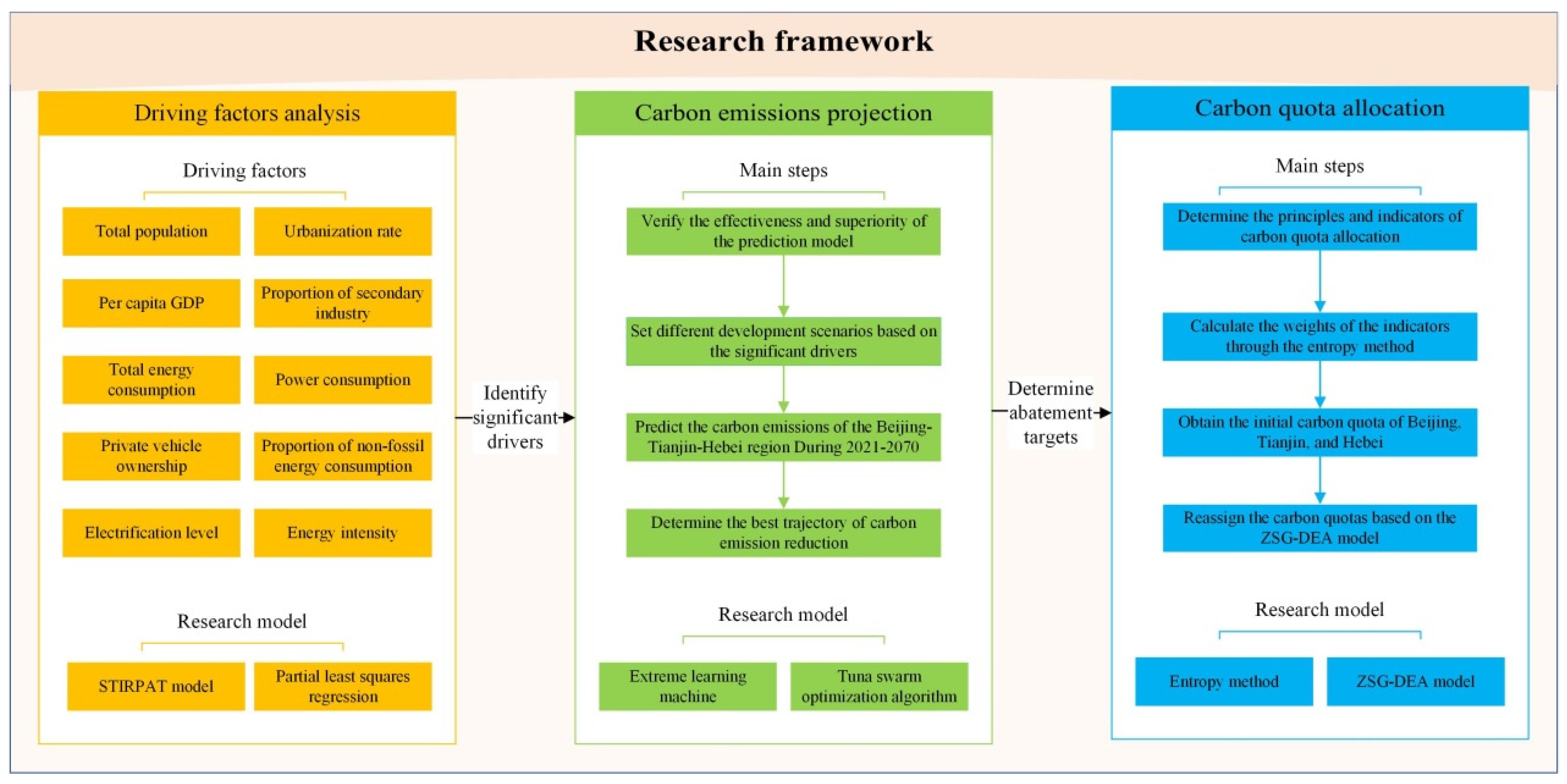
Figure 3.
TSO-ELM model structure diagram.
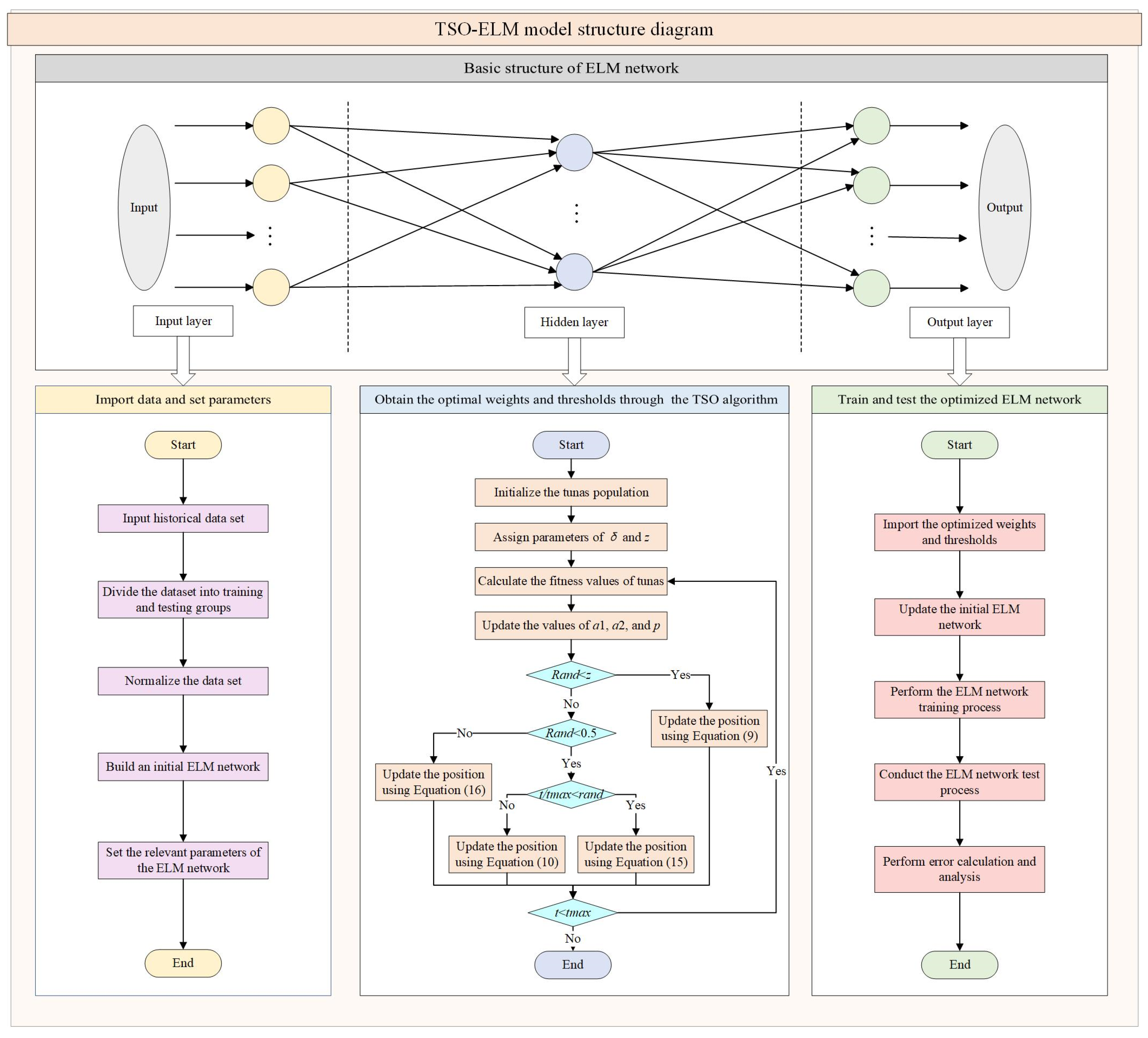
Figure 4.
Variations in power consumption in different areas under three patterns. (The symbols mark the power consumption of different regions in 2030 and 2070 under three patterns).
Figure 4.
Variations in power consumption in different areas under three patterns. (The symbols mark the power consumption of different regions in 2030 and 2070 under three patterns).
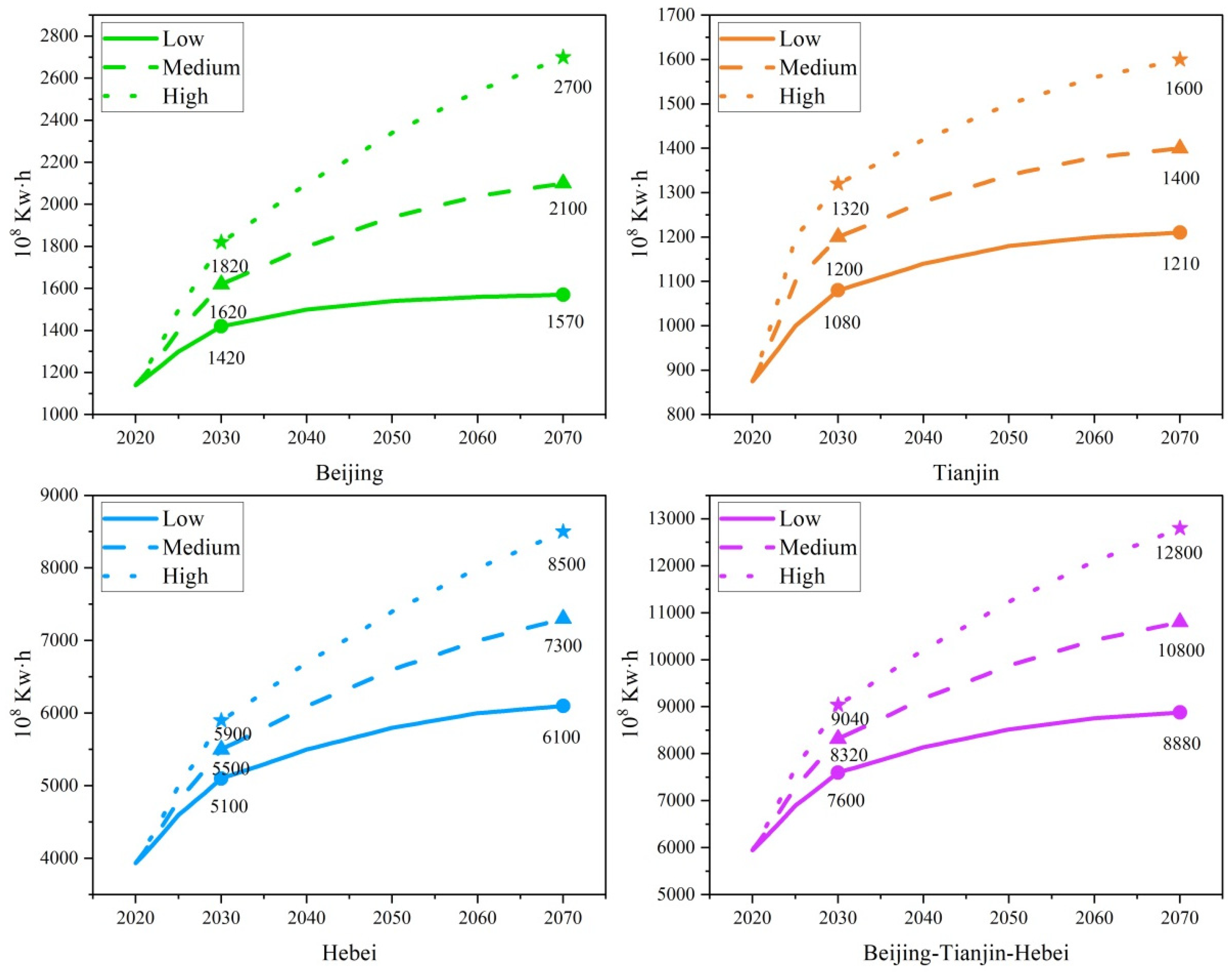
Figure 5.
Variations in private vehicle ownership in different areas under three patterns.
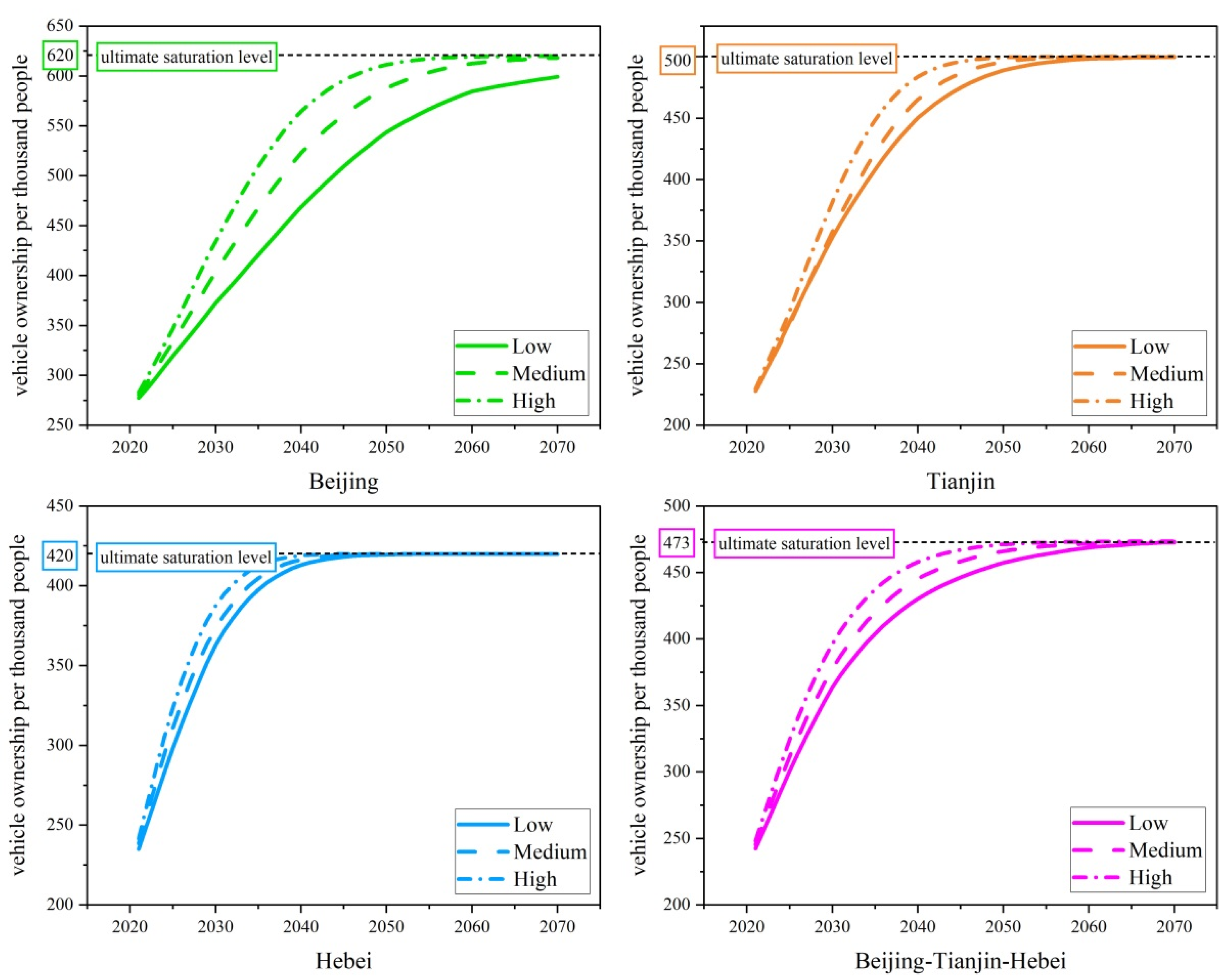
Figure 6.
Carbon emission trajectories and emission reduction in the BTH region under various scenarios.
Figure 6.
Carbon emission trajectories and emission reduction in the BTH region under various scenarios.
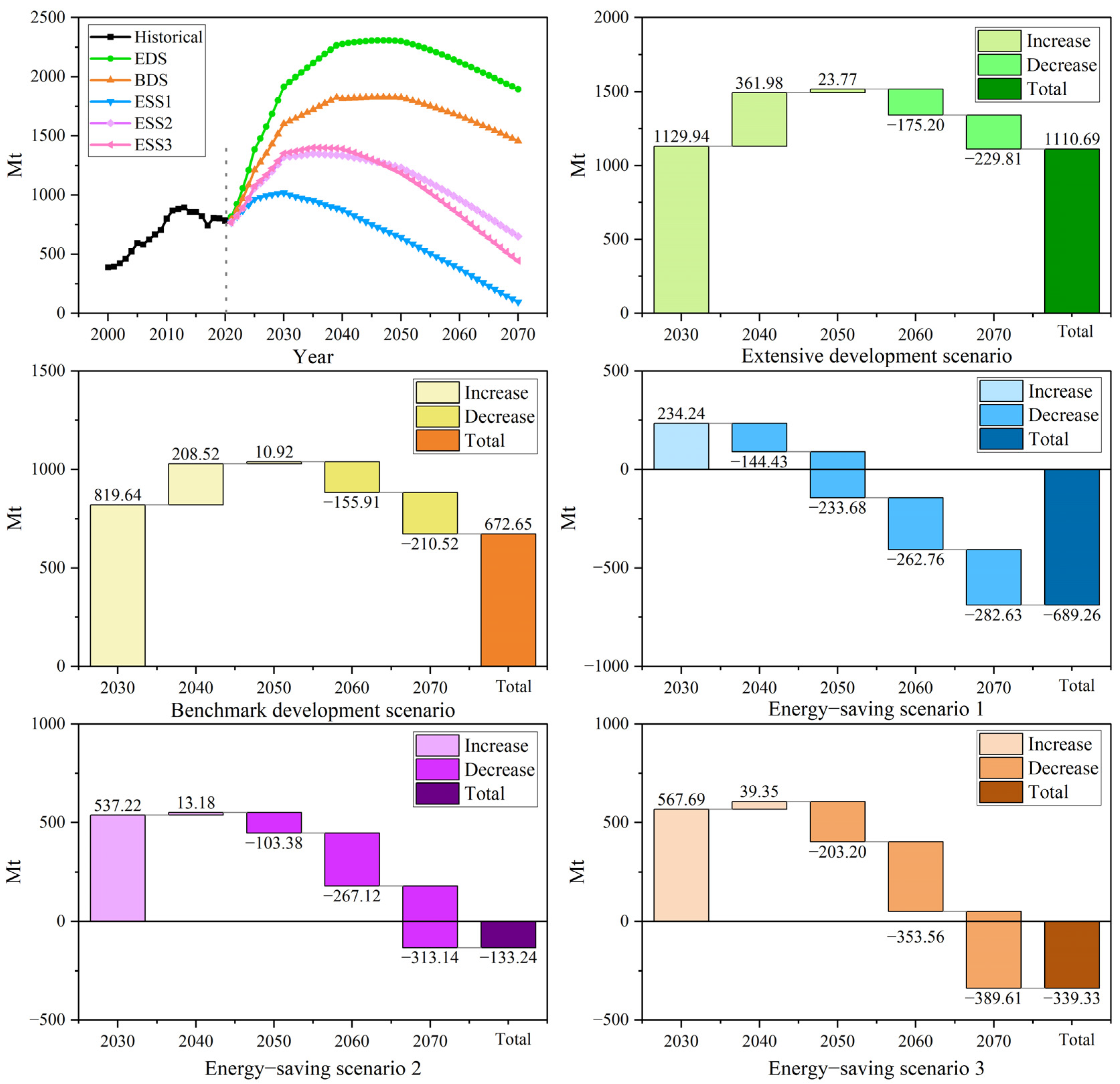
Table 1.
Summary of research methods on driving factors for carbon emission.
| Research Method | Research Author | Research Object | Applicability or Advantage |
|---|---|---|---|
| SDA | Duan et al. [14] | Drivers of carbon emissions in 112 countries | The SDA method is often combined with the input–output model, which can analyze the endogenous relationship between departments or variables [14]. |
| Luo et al. [15] | Influencing factors of carbon emissions in seven sub-sectors of China’s power industry | ||
| IDA | Yang et al. [16] | Driving factors of carbon emissions from residential construction industry in Henan Province, China | The calculation method of the IDA model is simple and easy to operate, and the decomposition result has no residual value [16]. |
| Sun et al. [17] | Driving forces of carbon emissions in 281 cities of China | ||
| Zou et al. [18] | Influencing indicators of carbon dioxide emissions in the Chinese power sector | ||
| STIRPAT | Shuai et al. [19] | Driving factors of carbon emissions in 125 countries | STIRPAT model is flexible in the selection of influencing factors and can evaluate the elastic coefficient of each factor [20]. |
| Wang et al. [20] | Impact factors of energy-related carbon emissions in Xinjiang, China. | ||
| Zhu et al. [21] | Drivers of implicit carbon emissions from the building industry in China | ||
| System dynamics | Zeng et al. [22] | Influencing factors of carbon emission in the Beijing–Tianjin–Hebei urban agglomeration | System dynamics can explore the complex relations of carbon-emission-related systems and dynamically analyze the influence of various factors on carbon emission [23]. |
| Li et al. [23] | Impact factors of carbon emissions in Hebei Province, China |
Table 2.
Description of variables.
| Element | Variable | Description | Unit |
|---|---|---|---|
| I | CE | Carbon emission | Mt |
| P | TP | Total population | 104 people |
| UR | Urbanization rate | % | |
| A | PGDP | Per capita gross domestic product | 104 CNY/person |
| TEC | Total energy consumption | 104 Tce | |
| PC | Power consumption | 108 Kw·h | |
| PV | Private vehicle ownership | Vehicles per thousand people | |
| T | EL | Electrification level | % |
| EI | Energy intensity | Tce/CNY 104 | |
| S | PSI | Proportion of secondary industry | % |
| NFEC | Share of non-fossil energy consumption | % |
Table 3.
Estimated coefficients of driving factors.
| Beijing | Tianjin | Hebei | BTH | |
|---|---|---|---|---|
| lnTP | 0.6140 | 0.5234 | 1.1547 | 1.0624 |
| lnUR | 2.4526 | 0.8639 | 0.1996 | 0.1928 |
| lnPGDP | −0.2365 | 0.0732 | 0.0884 | 0.0564 |
| lnTEC | 0.5493 | 0.1993 | 0.1967 | 0.2557 |
| lnPC | 0.0487 | 0.1235 | 0.1165 | 0.1366 |
| lnPV | 0.1752 | 0.0740 | 0.0389 | 0.0561 |
| lnEL | −0.1849 | −0.5590 | 0.1985 | 0.4218 |
| lnEI | 0.2233 | 0.0749 | 0.2229 | 0.2273 |
| lnPSI | 0.7699 | 0.2573 | 0.8200 | 0.8106 |
| lnNFEC | 0.0004 | 0.0021 | 0.0159 | 0.0101 |
Note: The confidence level is set to 95%.
Table 4.
VIP values of driving factors.
| Beijing | Tianjin | Hebei | BTH | |||||
|---|---|---|---|---|---|---|---|---|
| VIP Value | Sort | VIP Value | Sort | VIP Value | Sort | VIP Value | Sort | |
| lnTP | 0.8393 | 8 | 1.1060 | 2 | 1.0505 | 3 | 1.0334 | 3 |
| lnUR | 0.8394 | 7 | 1.0460 | 5 | 1.0449 | 4 | 1.0091 | 5 |
| lnPGDP | 0.8522 | 6 | 1.0183 | 6 | 1.0328 | 6 | 0.9817 | 6 |
| lnTEC | 0.8756 | 5 | 1.1301 | 1 | 1.1631 | 1 | 1.1602 | 1 |
| lnPC | 0.6873 | 10 | 1.0748 | 3 | 1.1384 | 2 | 1.0985 | 2 |
| lnPV | 0.8217 | 9 | 1.0679 | 4 | 1.0411 | 5 | 1.0137 | 4 |
| lnEL | 0.8758 | 4 | 0.8723 | 9 | 0.7317 | 10 | 0.8642 | 10 |
| lnEI | 0.8982 | 3 | 0.9538 | 7 | 0.8520 | 9 | 0.9256 | 8 |
| lnPSI | 1.0973 | 2 | 0.8799 | 8 | 0.9003 | 8 | 0.9804 | 7 |
| lnNFEC | 1.7812 | 1 | 0.7925 | 10 | 0.9663 | 7 | 0.8972 | 9 |
Note: The confidence level is set to 95%.
Table 5.
Error statistics of different prediction models.
| Prediction Models | BPNN | ELM | BA-ELM | TSO-ELM |
|---|---|---|---|---|
| MAE | 72.10 | 53.48 | 37.85 | 14.45 |
| MSE | 7084.08 | 4312.63 | 2250.52 | 360.84 |
| RMSE | 78.98 | 62.24 | 45.81 | 18.96 |
| MAPE, % | 9.16 | 6.84 | 4.42 | 1.86 |
Table 6.
Variations in total population in different areas under three patterns (104 people).
| Area | Pattern | 2020 | 2025 | 2030 | 2040 | 2050 | 2060 | 2070 |
|---|---|---|---|---|---|---|---|---|
| Beijing | Low | 2189 | 2280 | 2336 | 2390 | 2350 | 2300 | 2240 |
| Medium | 2189 | 2300 | 2360 | 2420 | 2460 | 2430 | 2390 | |
| High | 2189 | 2320 | 2380 | 2440 | 2480 | 2500 | 2490 | |
| Tianjin | Low | 1387 | 1419 | 1430 | 1436 | 1430 | 1410 | 1380 |
| Medium | 1387 | 1500 | 1550 | 1580 | 1600 | 1590 | 1570 | |
| High | 1387 | 1520 | 1570 | 1600 | 1620 | 1630 | 1625 | |
| Hebei | Low | 7464 | 7506 | 7308 | 6943 | 6600 | 6300 | 6000 |
| Medium | 7464 | 7550 | 7610 | 7560 | 7520 | 7480 | 7440 | |
| High | 7464 | 7570 | 7660 | 7730 | 7700 | 7680 | 7660 | |
| BTH | Low | 11,039 | 11,206 | 11,074 | 10,769 | 10,380 | 10,010 | 9620 |
| Medium | 11,039 | 11,350 | 11,520 | 11,560 | 11,580 | 11,500 | 11,400 | |
| High | 11,039 | 11,410 | 11,610 | 11,770 | 11,800 | 11,810 | 11,775 |
Table 7.
Variations in urbanization rate in different areas under three patterns (%).
| Area | Pattern | 2020 | 2025 | 2030 | 2040 | 2050 | 2060 | 2070 |
|---|---|---|---|---|---|---|---|---|
| Beijing | Low | 87.5 | 87.9 | 88.3 | 89.1 | 89.6 | 90.1 | 90.6 |
| Medium | 87.5 | 88.5 | 89.5 | 90.5 | 91.5 | 92.5 | 93.5 | |
| High | 87.5 | 89.0 | 90.5 | 92.0 | 93.5 | 95.0 | 96.5 | |
| Tianjin | Low | 84.7 | 85.5 | 86.0 | 87.3 | 88.0 | 88.5 | 89.0 |
| Medium | 84.7 | 86.0 | 87.0 | 88.0 | 89.0 | 90.0 | 91.0 | |
| High | 84.7 | 87.0 | 88.5 | 90.0 | 91.5 | 93.0 | 94.5 | |
| Hebei | Low | 60.1 | 62.2 | 65.5 | 72.5 | 76.0 | 78.0 | 80.0 |
| Medium | 60.1 | 65.0 | 70.0 | 77.0 | 81.0 | 84.0 | 87.0 | |
| High | 60.1 | 66.0 | 71.5 | 79.0 | 83.5 | 87.0 | 90.5 | |
| BTH | Low | 68.6 | 70.4 | 73.0 | 78.1 | 80.7 | 82.3 | 83.8 |
| Medium | 68.6 | 72.5 | 76.3 | 81.3 | 84.3 | 86.6 | 88.9 | |
| High | 68.6 | 73.5 | 77.7 | 83.2 | 86.7 | 89.5 | 92.3 |
Table 8.
Variations in GDP in different areas under three patterns (%).
| Area | Pattern | 2021–2025 | 2026–2030 | 2031–2040 | 2041–2050 | 2051–2060 | 2061–2070 |
|---|---|---|---|---|---|---|---|
| Beijing | Low | 4.0 | 3.5 | 3.0 | 2.5 | 2.0 | 1.0 |
| Medium | 5.0 | 4.5 | 4.0 | 3.5 | 3.0 | 2.0 | |
| High | 6.0 | 5.5 | 5.0 | 4.5 | 4.0 | 3.0 | |
| Tianjin | Low | 5.0 | 4.5 | 4.0 | 3.5 | 3.0 | 2.0 |
| Medium | 6.0 | 5.5 | 5.0 | 4.5 | 4.0 | 3.0 | |
| High | 7.0 | 6.5 | 6.0 | 5.5 | 5.0 | 4.0 | |
| Hebei | Low | 5.0 | 4.5 | 4.0 | 3.5 | 3.0 | 2.0 |
| Medium | 6.0 | 5.5 | 5.0 | 4.5 | 4.0 | 3.0 | |
| High | 7.0 | 6.5 | 6.0 | 5.5 | 5.0 | 4.0 | |
| BTH | Low | 4.6 | 4.1 | 3.7 | 3.2 | 2.7 | 1.7 |
| Medium | 5.6 | 5.1 | 4.7 | 4.2 | 3.7 | 2.7 | |
| High | 6.6 | 6.1 | 5.7 | 5.2 | 4.7 | 3.7 |
Table 9.
Variations in total energy consumption in different areas under three patterns (104 Tce).
| Area | Pattern | 2020 | 2025 | 2030 | 2035 | 2040 | 2050 | 2060 | 2070 |
|---|---|---|---|---|---|---|---|---|---|
| Beijing | Low | 6762 | 7800 | 8200 | 7900 | 7500 | 7000 | 6400 | 5700 |
| Medium | 6762 | 8050 | 8600 | 9000 | 8700 | 8300 | 7800 | 7200 | |
| High | 6762 | 8200 | 8900 | 9300 | 9500 | 9400 | 9200 | 8900 | |
| Tianjin | Low | 8105 | 8900 | 9300 | 9500 | 9200 | 8800 | 8300 | 7700 |
| Medium | 8105 | 9100 | 9600 | 9900 | 10100 | 9800 | 9400 | 8900 | |
| High | 8105 | 9300 | 9900 | 10,300 | 10,600 | 10,800 | 10,700 | 10,500 | |
| Hebei | Low | 32,783 | 35,400 | 36,500 | 37,000 | 36,300 | 35,200 | 33,500 | 31,000 |
| Medium | 32,783 | 36,400 | 38,000 | 39,000 | 39,500 | 38,900 | 38,000 | 36,600 | |
| High | 32,783 | 37,400 | 39,500 | 41,000 | 42,000 | 42,500 | 42,100 | 41,500 | |
| BTH | Low | 47,650 | 52,100 | 54,000 | 54,400 | 53,000 | 51,000 | 48,200 | 44,400 |
| Medium | 47,650 | 53,550 | 56,200 | 57,900 | 58,300 | 57,000 | 55,200 | 52,700 | |
| High | 47,650 | 54,900 | 58,300 | 60,600 | 62,100 | 62,700 | 62,000 | 60,900 |
Table 10.
Detailed scenario settings.
| Scenario | TP | UR | PGDP | TEC | PC | PV |
|---|---|---|---|---|---|---|
| EDS | High | High | High | High | High | High |
| BDS | Medium | Medium | Medium | Medium | Medium | Medium |
| ESS1 | Low | Low | Low | Low | Low | Low |
| ESS2 | Medium | Medium | Medium | Low | Low | Medium |
| ESS3 | High | High | High | Low | Low | High |
Table 11.
Peak time, peak value, and change rate of carbon emissions in the BTH region under various scenarios.
Table 11.
Peak time, peak value, and change rate of carbon emissions in the BTH region under various scenarios.
| Scenario | Peak Time | Peak Value (Mt) | Average Change Rate during the Pre-Peak Period (%) | Average Change Rate during the Post-Peak Period (%) |
|---|---|---|---|---|
| EDS | 2047 | 2306.34 | 4.18 | −0.85 |
| BDS | 2047 | 1824.87 | 3.25 | −0.98 |
| ESS1 | 2030 | 1018.41 | 2.69 | −5.63 |
| ESS2 | 2035 | 1349.04 | 3.74 | −2.05 |
| ESS3 | 2035 | 1400.99 | 4.01 | −3.20 |
Table 12.
Entropy values and weights of carbon quota allocation indicators.
| Indicator | Attribute | Principle | Entropy Value | Weight |
|---|---|---|---|---|
| Total population | Positive | Equality | 0.2879 | 0.1676 |
| Per capita GDP | Positive | Equality | 0.6174 | 0.0901 |
| Power consumption | Positive | Equality | 0.2759 | 0.1705 |
| Electrification level | Positive | Sustainability | 0.3710 | 0.1481 |
| Urbanization rate | Negative | Sustainability | 0.3305 | 0.1576 |
| Accumulated historical carbon emissions | Negative | Equality | 0.6302 | 0.0870 |
| Total energy consumption | Negative | Efficiency | 0.6309 | 0.0869 |
| Energy intensity | Negative | Efficiency | 0.6082 | 0.0922 |
Table 13.
Initial and final carbon quotas and allocation efficiency of Beijing, Tianjin, and Hebei.
| Area | Initial Efficiency | Initial Quota (Mt) | Final Efficiency | Final Quota (Mt) | Adjustment Amount (Mt) |
|---|---|---|---|---|---|
| Beijing | 1.0000 | 362.84 | 1.0000 | 482.16 | 119.32 |
| Tianjin | 1.0000 | 201.76 | 1.0000 | 268.12 | 66.36 |
| Hebei | 0.2039 | 453.81 | 1.0000 | 268.13 | −185.68 |
Disclaimer/Publisher’s Note: The statements, opinions and data contained in all publications are solely those of the individual author(s) and contributor(s) and not of MDPI and/or the editor(s). MDPI and/or the editor(s) disclaim responsibility for any injury to people or property resulting from any ideas, methods, instructions or products referred to in the content. |
© 2023 by the authors. Licensee MDPI, Basel, Switzerland. This article is an open access article distributed under the terms and conditions of the Creative Commons Attribution (CC BY) license (https://creativecommons.org/licenses/by/4.0/).
Share and Cite
MDPI and ACS Style
Zhang, S.; Dong, H.; Lu, C.; Li, W. Carbon Emission Projection and Carbon Quota Allocation in the Beijing–Tianjin–Hebei Region of China under Carbon Neutrality Vision. Sustainability 2023, 15, 15306. https://doi.org/10.3390/su152115306
AMA Style
Zhang S, Dong H, Lu C, Li W. Carbon Emission Projection and Carbon Quota Allocation in the Beijing–Tianjin–Hebei Region of China under Carbon Neutrality Vision. Sustainability. 2023; 15(21):15306. https://doi.org/10.3390/su152115306
Chicago/Turabian StyleZhang, Shuohua, Hanning Dong, Can Lu, and Wei Li. 2023. "Carbon Emission Projection and Carbon Quota Allocation in the Beijing–Tianjin–Hebei Region of China under Carbon Neutrality Vision" Sustainability 15, no. 21: 15306. https://doi.org/10.3390/su152115306
Note that from the first issue of 2016, this journal uses article numbers instead of page numbers. See further details here.