Environmental Damage of Different Waste Treatment Scenarios by Considering Avoided Emissions Based on System Dynamics Modeling

Abstract

This study aims to develop a comprehensive model for life cycle assessment and environmental damage cost calculations considering avoided emissions in different waste management scenarios using the system dynamics (SD) approach. Our analysis reveals that under the business-as-usual (BAU) scenario for the period 2020–2050, the total net greenhouse gas (GHG) emissions reach 12.5 Mt, with the highest environmental damage cost being USD 689 million. In contrast, an integrated management strategy encompassing recycling, composting, anaerobic digestion, and incineration results in a 195% reduction in net GHG emissions compared to the BAU Scenario. Concurrently, the environmental damage cost drops to USD 277 million, incorporating USD 347 million in savings, leading to a net environmental damage cost of USD −71 million. The findings affirm that accounting for emissions avoided across various treatment methods offers a more accurate estimate of environmental damage costs. Additionally, policies centered on integrated waste management are more likely to achieve sustainability. The study also demonstrates the utility of the SD approach in providing a holistic view of waste management systems and in evaluating the effectiveness of various policy strategies for sustainable waste management.

1. Introduction

Solid waste management is one of the most urgent and significant issues in the world. The importance of this issue can be perceived from the fact that twelve out of seventeen United Nations’ Sustainable Development Goals are directly related to solid waste [1]. With population growth, rapid urbanization, and economic development, municipal solid waste generation rates are steadily increasing, and coupled with the feeble performance of managers in choosing the right treatment, this can worsen such conditions, especially in developing and emerging countries [2,3,4]. It is widely documented that insufficient waste management negatively affects air, soil, and water quality, as well the climate, public health, and, ultimately, the economy [5,6,7].

Many countries are looking for an appropriate waste management system to reduce the volume of waste and the related environmental impacts [8]. A capable and sustainable waste management system is vital both for human health and environmental protection [9]. Undoubtedly, sustainable waste management is an innovative solution for solid waste treatment to improve practicality and to meet the goals of reduction, reuse, recycling, and treatment strategies with the lowest environmental damage cost [10]. Recycling, composting, anaerobic digestion, and incineration are suitable options for waste treatment [11]. However, different treatment methods have different emissions and environmental impacts [12]. The life cycle assessment (LCA) and life cycle inventory (LCI) methods have been broadly used as tools to estimate the environmental performance of waste management systems [13]. The life cycle impact assessment method based on endpoint (LIME) assists decision-makers in selecting the best option with a minimal impact on the environment by quantifying the life cycle environmental impacts of different waste treatment options [14].

In recent years, researchers have focused more on assessing environmental damage costs as a concept of environmental economics or external environmental costs. In this regard, Dijkgraaf and Vollebergh [15] compared environmental damage costs caused by landfilling and incineration and found that converting waste to energy is better than transferring it to landfill. Yi et al. [16] applied the LIME model to investigate municipal solid waste management scenarios based on the midpoint and endpoint approaches. Liu et al. [17] investigated the environmental damage cost of different waste treatment scenarios using the LIME3 method. The analysis showed that fermentation has the least and landfills have the most environmental damage cost.

These studies appraised the environmental damage cost based on the emissions of different waste treatment methods. However, the avoided emissions from the waste treatment products that could potentially offset GHG emissions were not considered. Calculating avoided emissions due to waste-based products shows a more accurate view of the environmental effects of waste management and can offset GHG emissions from other sectors and lead to net negative emissions from the waste management sector [18]. Amaral et al. [19] stated that the use of appropriate waste management methods could transform the waste management system in a country from a GHG producer to a net-zero GHG producer.

The open dumping of waste (both controlled and uncontrolled) is the ultimate option for collected waste in Iran, which poses lack of land and environmental and health challenges for city residents [20]. The local government has founded a policy action known as Vision 2030 to manage the massive generation of waste and minimize its disposal for economic and environmental benefits. The available relevant solutions concentrate mostly on evaluating the environmental damage from prevailing treatment techniques, such as landfilling [21], incineration [22], and biochemical treatment [23], as well as an integrated waste management system [24].

To investigate the consequences of waste treatment methods, it is necessary to select acceptable approaches and develop a comprehensive model. Simulation models, as appropriate tools for scenario analysis, can help decision-makers in the decision making and performance review of waste management policies [25]. System dynamics (SD) is an analysis and simulation methodology of temporal behavior that can help investigate the structure, interactions, and behavior styles of complex systems and assess their impacts in a comprehensive manner [26]. The SD approach has been widely used to study the waste management sector, such as waste separation [27,28], analysis of new policies [29,30,31], waste generation prediction [32,33], and converting waste to energy [34].

However, to our knowledge, the existing literature lacks a comprehensive system dynamics model to evaluate the life cycle of waste management systems, particularly in developing countries. To address this gap, a comprehensive waste management model has been developed to assess the life cycle based on the endpoint approach and the environmental damage cost using Vensim PLE software (Ventana Systems, USA, 2015). The proposed model also takes into account the avoided emissions of valuable products using different treatment methods to investigate the emissions mitigation potential. The developed model can be used as a reference for other places facing the problem of waste management. The innovation of this research is due to the development of a comprehensive waste flow model and quantifying the environmental damage cost by considering avoided emissions for the analysis of different scenarios.

Household waste is an important focus of this study because it includes the composition of heterogeneous resources, which can potentially be recovered if proper separation, collection, and treatment methods are accomplished. The model investigates all separated recyclable and residual waste streams, as well as representative technologies for the treatment of individual waste streams. The model is designed to be extensible, allowing for the future incorporation of more complex system dynamics (SD) variables, including socioeconomic and environmental factors and potential policy-related feedback loops.

2. Materials and Methods

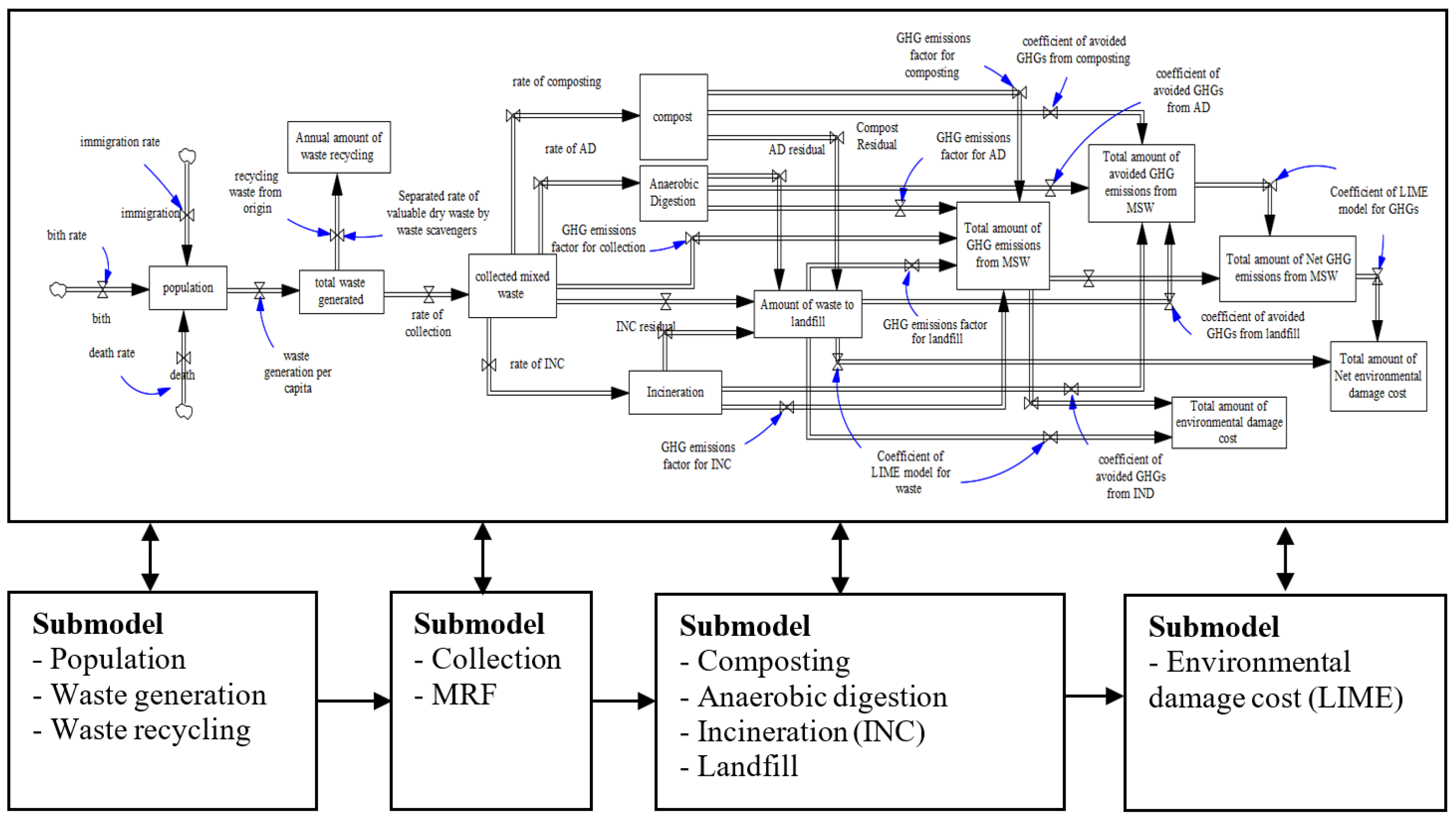
2.1. SD Model

The system dynamics (SD) model was developed through a series of steps outlined in the following sections. First, the structure of the model is explained in Section 2.2. Second, greenhouse gas (GHG) emissions and avoided GHGs from the waste stream are presented in Section 2.3. Third, the LIME model, which is used to calculate environmental damage costs, is described in Section 2.4. Fourth, in Section 2.5, the model’s quantification and implementation were conducted using data on Alborz Province, which is located in Iran. In addition, various scenarios were developed that are closely aligned with Alborz Province’s waste management strategies and that considered both local structural factors and international guidelines.

2.2. Model Structure

The SD model has been used in articles to analyze waste streams to investigate environmental damage cost scenarios using an equation-based model [34,35,36,37]. Figure 1 characterizes the conceptual system dynamics model of a waste stream. The arrows in the figure exhibit the stream of information between the subsystems. The waste stream subsystems are depicted using the system dynamics diagram model [38], in which a rectangular box characterizes a stock, a pipe arrow pointing to a reservoir characterizes an inflow, a pipe arrow out of a stock characterizes outflows, valves on the pipes control the flows, clouds show sources/sinks, and each connected arrow shows a causal relationship. The proposed model is initially an open-loop, unidirectional model without significant feedback loops, a feature also observed in other solid waste models in the existing literature [34,35,36,37]. Even so, the use of SD as a modeling tool remains reliable, especially in large systems with multiple variables that interact in complex ways, not necessarily following linear relationships. Generally, both closed-loop and open-loop system simulations are recognized as reliable methods for gaining an overview of dynamic systems [39].

The presented model includes four subsections: (1) waste generation and recycling, (2) collection, (3) waste treatment, and (4) the LIME model. The model is constructed in such a way that the output(s) of a previous module is transformed into the input of the next module following a main direction of computation. The details of the model are explained below.

The waste generation submodule estimates the information on population growth and the total waste generated and waste composition. The submodule of recycling refers to the amount of valuable dry waste. The variable “recycling waste from the origin” shows the amount of separated dry waste at the source at any time and affects the “separated rate of valuable dry waste by waste scavengers”. The waste collection submodule represents the amount of collected waste (i.e., mixed waste) in the same period as that obtained by removing recycled waste from the origin and recycled waste by scavengers from the total waste generated. The material recycling facility (MRF) submodule refers to the amount of valuable dry wastes that are separated at the receiving site.

Waste treatment and disposal submodels represent the final fate of waste through the process of composting, anaerobic digestion, waste incineration, and landfilling. Solid waste may be directly transferred to the landfill or enter other processes according to the type of waste. In addition, each of the processes also has residual materials that eventually enter the landfill. The amount of net GHGs in each submodule is calculated using the GHG emissions (direct emissions from processes and input materials) and avoided GHGs (production of different products and savings from input material). According to the GHG emissions factor per liter of fuel required, the amount of GHG emissions using the collection and transportation of waste is determined. The LIME submodel refers to the environmental damage cost according to the amount of waste sent to the landfill and the GHG emissions in each method. The full details on the submodels (Figures S1–S9) and the amount of parameters used along with their sources (Tables S1 and S2) are provided in the Supplementary Materials.

2.3. GHGs in Waste Stream

The direct emission of GHGs is calculated using the relevant coefficients in the processes of collection [40], recycling [41], composting [42], anaerobic digestion [41,43], incineration [35,37], and landfill [34,43] with Equations (1)–(6), respectively. All of the parameters for the equations are mentioned in the list of abbreviations.

$$GH{G}_{DEM}^{COL}=(F{U}_{RG}^{COL}\times E{F}_{C{O}_2}^{COL})+(F{U}_{RG}^{COL}\times E{F}_{C{H}_4}^{COL}\times GW{P}_{C{H}_4})$$

(1)

$$GH{G}_{DEM}^{RC}=V_{M,P,PL}^{RC}\times E{F}_{C{O}_2}^{RC}$$

(2)

$$GH{G}_{DEM}^{COM}=(V_{OW}^{COM}\times E{F}_{C{H}_4}^{COM}\times GW{P}_{C{H}_4})+(V_{OW}^{COM}\times E{F}_{N_{2}O}^{COM}\times GW{P}_{N_{2}O})$$

(3)

$$GH{G}_{DEM}^{AD}=(V_{OW}^{AD}\times E{F}_{C{H}_4}^{AD}\times GW{P}_{C{H}_4})$$

(4)

$$GH{G}_{DEM}^{INC}=(MW\times V_{P,PL,}^{INC}{}_{NVD}\times CCW\times FCF\times CE)+(V_{P,PL,}^{INC}{}_{NVD}\times {\mathrm{EF}}_{{\mathrm{N}}_2\mathrm{O}}^{\mathrm{INC}}\times GW{P}_{N_{2}O})$$

(5)

$$GH{G}_{DEM}^{LF,LEF}=(V_{OW}^{LF,LEF}\times EE{F}_{C{H}_4,OW}^{LF,LEF}+V_D^{LF,LEF}\times EE{F}_{C{H}_4,D}^{LF,LEF})*GW{P}_{C{H}_4}$$

(6)

Based on the amount of recycled waste, compost fertilizer, and electricity produced, avoided GHGs are calculated based on the relevant coefficients in the processes of recycling [36], composting [44,45], anaerobic digestion [44,46], incineration, and landfilling [47] using Equations (7)–(11).

$$GH{G}_{AV}^{RC}=(V_M^{RC}\times C{F}_{C{O}_2}^M)+(V_P^{RC}\times C{F}_{C{O}_2}^P)+(V_{PL}^{RC}\times C{F}_{C{O}_2}^{PL})$$

(7)

$$GH{G}_{AV}^{COM}={(\mathrm{N}}_{SV}^{COM}\times {\mathrm{CF}}_{{\mathrm{CO}}_2}^{\mathrm{UR}}{)+(\mathrm{P}}_{SV}^{COM}\times {\mathrm{CF}}_{{\mathrm{CO}}_2}^{\mathrm{DAP}}{)+(\mathrm{K}}_{SV}^{COM}\times {\mathrm{CF}}_{{\mathrm{CO}}_2}^{\mathrm{SOP}}{)+(\mathrm{C}}_{SV}^{COM}\times {\mathrm{CF}}_{{\mathrm{CO}}_2}^{\mathrm{HU}})$$

(8)

$$GH{G}_{AV}^{AD}={(\mathrm{N}}_{SV}^{AD}\times {\mathrm{CF}}_{{\mathrm{CO}}_2}^{\mathrm{UR}}{)+(\mathrm{Ph}}_{SV}^{AD}\times {\mathrm{CF}}_{{\mathrm{CO}}_2}^{\mathrm{DAP}}{)+(\mathrm{K}}_{SV}^{AD}\times {\mathrm{CF}}_{{\mathrm{CO}}_2}^{\mathrm{SOP}}{)+(\mathrm{C}}_{SV}^{AD}\times {\mathrm{CF}}_{{\mathrm{CO}}_2}^{\mathrm{HU}}{)+(\mathrm{EL}}_{PR}^{AD}\times C{F}_{C{O}_2}^{EL})$$

(9)

$$GH{G}_{AV}^{AD}={(\mathrm{EL}}_{PR}^{INC}\times C{F}_{C{O}_2}^{EL})$$

(10)

$$GH{G}_{AV}^{LFE}={(\mathrm{EL}}_{PR}^{LFE}\times C{F}_{C{O}_2}^{EL})$$

(11)

Indirect GHG emissions and avoided GHGs are determined according to the coefficients of fuel and electricity consumption in the processes of recycling [48], composting [49], anaerobic digestion [50], incineration [51], and landfilling [52], as well as, the coefficient of GHG emissions due to the consumption of electricity [53], petrol [54], and diesel [55].

Considering the different energy and fuel consumptions in various treatment methods, the amount of GHG emissions because of the consumption of input materials is calculated using Equations (12)–(16).

$$GH{G}_{IEM}^{RC}=E{L}_{RQ}^{RC}\times C{F}_{C{O}_2}^{EL}$$

(12)

$$GH{G}_{IEM}^{COM}=(F{U}_{RQ}^{COM}\times C{F}_{C{O}_2}^{FU})+(F{U}_{RQ}^{COM}\times C{F}_{C{H}_4}^{FU}\times GW{P}_{C{H}_4})+(E{L}_{RQ}^{COM}\times C{F}_{C{O}_2}^{EL})$$

(13)

$$GH{G}_{IEM}^{AD}=(E{L}_{RQ}^{AD}\times C{F}_{C{O}_2}^{EL})$$

(14)

$$GH{G}_{IEM}^{INC}=(E{L}_{RQ}^{INC}\times C{F}_{C{O}_2}^{EL})$$

(15)

$$GH{G}_{IEM}^{LF,LFE}=(F{U}_{RQ}^{LF,LFE}\times C{F}_{C{O}_2}^{FU})+(F{U}_{RQ}^{LF,LFE}\times C{F}_{C{H}_4}^{FU}\times GW{P}_{C{H}_4})+(E{L}_{RQ}^{LF,LFE}\times C{F}_{C{O}_2}^{EL})$$

(16)

Because of diverting waste from landfills, the avoided GHGs due to the non-use of raw materials compared to the BAU Scenario is calculated with Equations (17)–(20).

$$GH{G}_{IAV}^{RC}=(F{U}_{SV}^{RC}\times C{F}_{C{O}_2}^{FU})+(F{U}_{SV}^{RC}\times C{F}_{C{H}_4}^{FU}\times GW{P}_{C{H}_4})+(E{L}_{SV}^{RC}\times C{F}_{C{O}_2}^{EL})$$

(17)

$$GH{G}_{IAV}^{COM}=(F{U}_{SV}^{COM}\times C{F}_{C{O}_2}^{FU})+(F{U}_{SV}^{COM}\times C{F}_{C{H}_4}^{FU}\times GW{P}_{C{H}_4})+(E{L}_{SV}^{COM}\times C{F}_{C{O}_2}^{EL})$$

(18)

$$GH{G}_{IAV}^{AD}=(F{U}_{SV}^{AD}\times C{F}_{C{O}_2}^{FU})+(F{U}_{SV}^{AD}\times C{F}_{C{H}_4}^{FU}\times GW{P}_{C{H}_4})+(E{L}_{SV}^{AD}\times C{F}_{C{O}_2}^{EL})$$

(19)

$$GH{G}_{IAV}^{INC}=(F{U}_{SV}^{INC}\times C{F}_{C{O}_2}^{FU})+(F{U}_{SV}^{INC}\times C{F}_{C{H}_4}^{FU}\times GW{P}_{C{H}_4})+(E{L}_{SV}^{INC}\times C{F}_{C{O}_2}^{EL})$$

(20)

Finally, the net amount of GHGs is calculated based on Equation (21) through the difference between the total emission of GHGs because of different treatment methods and consumed input materials, and the total avoided GHGs through the production of products and diversion of waste from landfill using different methods. The value of the coefficients in the equations along with their sources are provided in the Supplementary Materials (Table S2).

$$ne{t}^{}GH{G}^{Tech}=(GH{G}_{DEM}^{Tech}+GH{G}_{IEM}^{Tech})-(GH{G}_{AV}^{Tech}+GH{G}_{IAV}^{Tech})$$

(21)

2.4. LIME Model

The LIME model was expanded with the support of Japan’s Ministry of Economy, Trade, and Industry (METI) to reflect the environmental and social conditions [56,57]. After improving LIME1 and LIME2, LIME3 was developed and has been used to assess the environmental impacts on a global scale since 2016 [58]. This method includes all of the main steps of a life cycle impact assessment, including characterization, damage assessment, and weighting [59].

After determining the inventory data in the SD model of the waste management system, three indicators are used to convert the impact category into damage cost and the final single index. The damage factor (DF) index is used to assess the amount of damage to each of the four conservation issues, namely, “human health”, “social assets”, “biodiversity”, and “primary productivity”. The weighting factor/coefficient (WF) is used to merge the damage rate of the four protection objectives and convert them into a single index. The WF values for each country are given in the LIME model. The integration factor index (IF) is obtained by multiplying the damage factor (DF) by the weight factor (WF). Then, the total environmental damage cost (single index) I is determined using Equations (22) and (23) [17]. The corresponding coefficients of the LIME model is obtained from its official database (https://lca-forum.org/english/lime/, accessed on 1 November 2018).

$$I={\displaystyle \sum {}_{\mathrm{Im}pact}{\displaystyle \sum {}_{safe}}}{\displaystyle \sum {}_x}Inv(X)*DF(Safe,X)*EV(Safe)$$

(22)

$$={\displaystyle \sum {}_{\mathrm{Im}pact}}{\displaystyle \sum {}_x}Inv(X)*IF(X)$$

(23)

where Inv (X) indicates the inventory data of contaminant X; DF (Safe, X) indicates the damage factor caused by the conversion of “safe” subjects with contaminant X; and EV (Safe) is the economic value conversion factor due to the damage of one unit of the “safe” conservation area. The values of the model parameters are presented in the Supplementary Materials (Table S1).

This study presents environmental damage through both emissions and net emissions. Thus, LCIA outcomes are indicated as “net emissions”, representing “system emissions from each scenario” minus “avoided emissions”. System emissions include common GHG emissions from waste processes and input material. Avoided emissions include GHG emissions savings from the production of different products and use of different input materials.

2.5. Model Quantification, Implementation, and Scenario Settings

We applied the system dynamics model exhibited in Figure 1 in the educational version of Vensim PLE software (Ventana Systems USA, 2015). We determined the SD model based on the models in [34,35,36,37]; in addition, we added the LIME model that was used in the work of Liu et al. (2021) [17] to calculate the environmental damage cost. Details on the model and the equations in the model are supplied in the Supplementary Materials (Figures S1–S9; Tables S1 and S2). The default SD model indicates a BAU Scenario, or the base case. Also, to test the model and compare its results with the base scenario, several other scenarios were also implemented. Alborz Province was selected as the case study due to its programs for sustainable waste management. The study period was from 2020 to 2050, since 2050 is the key year for zero global emissions.

The National Waste Management Law of Iran and its executive regulations state that all Iranian municipalities must provide a Municipal Plan of Integrated Solid Waste Management, with specified objectives for waste separation and waste destination. Therefore, the scenarios were expanded to consider plans for waste management strategies for the nearby Alborz Municipal Waste Management Organization, and it took into account local structural factors, as well as international guidelines. Six scenarios were determined to simulate the outcome of the desired programs of the organization based on these purposes (

Table 1. Description of the scenarios’ design.

Scenario	Name	Purposes	Assumptions
BAU Scenario	Unmanaged landfilling	Investigating the environmental effects of continuing the current conditions	Continuation of the current situation, in which only 10% of the valuable dry waste is separated at the source and the rest is disposed of in an unmanaged landfill.
Scenario S1	Recycling	Predicting the plan of municipalities regarding source separation to achieve sustainable development	Increase in the participation of citizens in valuable dry waste separation from 10% in the current situation to 70% starting in 2035.
Scenario S2	Sanitary landfilling	Reducing GHG emissions, electricity production	Change from an unmanaged landfill in the BAU Scenario to a sanitary landfill for energy extraction.
Scenario S3	Composting	Reducing the landfill, further exploitation of the landfill site	Application of the compost process to 50% of the organic waste in 2023 to modify the effect of the organic waste treatment’s structure and the optimization of the treatment’s structure.
Scenario S4	Anaerobic digestion	Reducing the landfill, further exploitation of the landfill site	Application of the anaerobic digestion process to 50% of the organic waste in 2025 to modify the effect of the organic waste treatment’s structure and the optimization of the treatment’s structure.
Scenario S5	Incineration	Management of residual dry waste and energy production	Application of incineration to residual dry waste in 2025.
Scenario S6	ISWM	Taking advantage of all scenarios	Simultaneous implementation of the recycling, composting, anaerobic digestion, and incineration scenarios for the integrated management of all waste.

). The variables and equations related to the implementation of the scenarios are shown in the Supplementary Materials (Table S3).

2.6. Model Validation Test

The created model was tested for its structural validation and behavior validation [60,61]. Structural validity was evaluated by conducting a (1) dimensional consistency test and an (2) extreme condition test. The validation results for the model are provided in the Supplementary Materials (Figures S10–S13).

The behavioral validation of an SD model with historical data was conducted using the mean absolute error (MAE), mean squared error (MSE), root mean squared error (RMSE), and mean absolute percentage error (MAPE) based on Equations (24)–(27) [62,63]. The validation is performed by comparing the relative error between the actual and estimated value. According to the available data, the population and total waste generated variables were used for the validation test in the period of 2011 to 2020. The error between the actual and estimated values is shown in

Table 2. Validity test for the total population and total waste generated.

Year	Total Population (Ten Thousand Persons)			Total Waste Generated (Million Tons)
	Actual	Estimated	Error	Actual	Estimated	Error
2011	241.25	241.25	0.00	0.557	0.567	−0.009
2012	245.70	246.56	−0.86	0.602	0.592	0.010
2013	250.20	252.15	−1.95	0.634	0.619	0.015
2014	254.80	257.91	−3.11	0.667	0.647	0.020
2015	259.40	264.05	−4.65	0.664	0.676	−0.012
2016	271.24	270.39	0.85	0.606	0.706	−0.100
2017	276.60	276.71	−0.11	0.609	0.722	−0.112
2018	281.60	282.97	−1.36	0.619	0.730	−0.111
2019	286.50	288.67	−2.17	0.643	0.737	−0.094
2020	291.30	293.80	−2.50	0.697	0.742	−0.045

.

$$MAE=\frac{{\displaystyle \sum _{i=1}^n\left|A_t-E_t\right|}}{n}$$

(24)

$$MSE=\frac{{\displaystyle \sum _{i=1}^n{(A_t-E_t)}^{{}^2}}}{n}$$

(25)

$$RMSE=\sqrt{\frac{{\displaystyle \sum _{i=1}^n{(A_t-E_t)}^{{}^2}}}{n}}$$

(26)

$$MAPE=\frac{{\displaystyle \sum _{i=1}^n\left|\frac{A_t-E_t}{A_t}\right|}}{n}\times 100$$

(27)

where A_t is the actual observations, F_t is the estimated value, and n is the number of data.

The values for the MAE, MSE, and RMSE for the population were 1.76, 4.94, and 2.22, respectively, and for the total waste were 0.053, 0.005, and 0.068, respectively (

Table 3. Model validation results.

Variable	MAE	MSE	RMSE	MAPE (%)
Population	1.76	4.94	2.22	0.66
Total waste generated	0.053	0.005	0.068	8.43

). The MAPE results are classified into four types: excellent (MAPE < 10), good (MAPE = 10), acceptable (MAPE = 20–50), and unacceptable (MAPE > 50) [64]. The values for the MAPE for the population and total waste were 0.66% and 8.43%, respectively, which indicate an excellent prediction value (Table 3). Graphs of the actual and estimated values for the population and total waste variables are shown in Figures S14 and S15 in the Supplementary Materials.

3. Results and Discussion

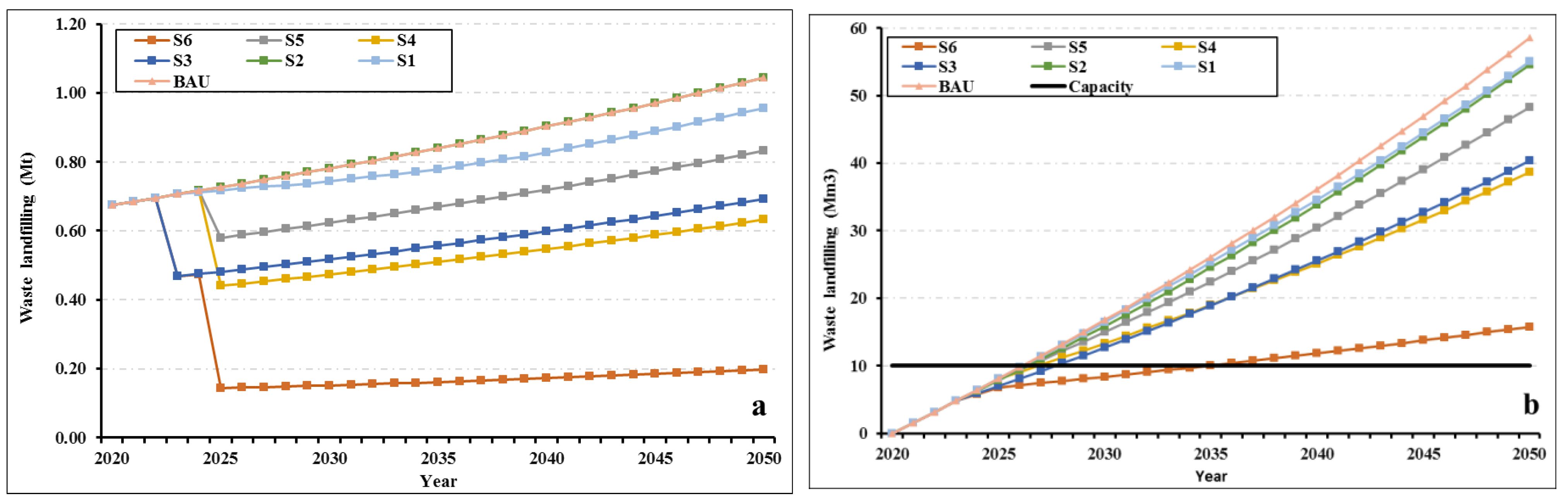
3.1. Amount of Waste Sent to Landfill

Figure 2a demonstrates the amount of waste sent to the landfill in each scenario, which depends on the recycling percentage, composting, anaerobic digestion, and incineration rates (auxiliary variables). The amount of waste sent to the landfill in the BAU Scenario (unmanaged landfill) and S2 (sanitary landfill) are the same, since the remaining waste after recycling dry waste is transferred to the landfill in both scenarios. The amount of waste landfilling in these two scenarios increased by 54.3% during the simulation periods, rising from 0.68 Mt in 2020 to 1.04 Mt in 2050. The continual population growth and urbanization over the past decades caused a significant increase in waste production [65,66,67].

The difference in the total amount of waste sent to the landfill during the simulated periods when comparing the BAU Scenario and Scenario S1 is 1.58 Mt, which indicates a 6% decrement, considering only the difference perceived in the last semester of the simulations, and it is feasible to apperceive a reduction of 0.08 Mt, representing an 8.12% reduction. The increase in waste separation caused an extra amount of 1.6 Mt of recycled waste comparing the BAU Scenario during the simulation period. The implementation of each of the scenarios leads to the diversion of waste from the landfill; therefore, with the implementation of Scenario S3 starting from 2023 and Scenarios S4 and S5 from 2025, the amount of waste sent to the landfill decreases significantly. The composting (Scenario S3), anaerobic digestion (Scenario S4), and incineration (Scenario S5) processes compared to the BAU Scenario leads to a decrease of 31.1%, 34.2%, and 17.6% in waste landfilling. The least amount of waste landfilling was observed with the simultaneous implementation of the recycling, composting, anaerobic digestion, and incineration programs in Scenario S6, which indicated a 71.92% decrement.

The total amount of waste sent to the landfill during the simulation period was 26.25 Mt, 24.67 Mt, 26.25 Mt, 18.09 Mt, 17.28 Mt, 21.63 Mt, and 7.37 Mt for the BAU Scenario, Scenario S1, Scenario S2, Scenario S3, Scenario S4, Scenario S5, and Scenario S6, respectively. Based on the studies carried out in the only active landfill site in Alborz Province, Halghedare [68], the remaining capacity of this landfill center is estimated at 10 Mm³. The required capacity based on the waste sent to the landfill during the simulation period for the BAU Scenario, Scenario S1, Scenario S2, Scenario S3, Scenario S4, Scenario S5, and Scenario S6 is 58.52 Mm³, 55.07 Mm³, 54.58 Mm³, 40.40 Mm³, 38.66 Mm³, 48.30 Mm³ and 15.79 Mm³, respectively, which is more than the remaining capacity for all scenarios, with the difference that in the BAU Scenario, Scenario S1, Scenario S2, Scenario S4, and Scenario S5, the landfill capacity will be reached in 2027, while for Scenario S3 and Scenario S6 it will be in 2028 and 2035, respectively (Figure 2b).

3.2. GHGs in Different Scenarios

The net GHG emissions were calculated using the difference between the GHG emissions and avoided GHGs. The net GHG emissions caused by the scenarios of recycling (S1), sanitary landfilling (S2), composting (S3), anaerobic digestion (S4), and incineration (S5) from 2020 to 2050 are represented in Figure 3. During 2020–2050, Scenario S6 (IWMS) had the highest net GHG emissions mitigation potential, followed by Scenario S4. Notably, the net GHG emissions under Scenarios S6 and S4 were negative after implementation, representing that the waste sector acts as a considered GHGs sink. The key reason for the negative net GHG emissions (i.e., GHGs sink) is the diversion of waste from landfill that not only leads to the reduction of GHG emissions but also avoids GHGs through the products of waste treatment processes that can mitigate the effect of GHG emissions.

The net GHG emissions under the BAU Scenario and Scenario S1 demonstrate an increasing trend during 2020–2050 from approximately 0.33 Mt in 2020 to 0.52 Mt and 0.45 Mt in 2050, respectively (representing a 54% and 35% increase, respectively). This increase is due to the transfer of organic waste to traditional landfills and their decomposition under anaerobic conditions, which is one of the most important human sources of GHG emissions and contributes to global warming [69,70].

The net GHG emissions with the implementation of Scenarios S2 and S3 in 2023 reached 0.06 and 0.14 Mt, respectively, with 83% and 58% reductions compared to 2020, which compared to the BAU Scenario (0.35 Mt in 2023) decreased by 83% and 60%, respectively. However, the net GHG emissions in Scenarios S2 and S3 from 2023 to 2050, with an increase of 48%, will reach 0.09 and 0.21 Mt, respectively, because of the increase in waste production starting from 2023. Moghadam et al. [71] showed that, assuming the opening of a landfill site in 2012 and considering the 20-year planned period for its use, the total GHG emissions from sanitary landfills in Iran in 2032 is equal to 3,844,000 Mg/year. The use of gas collection systems in sanitary landfills is suggested as the best option to prevent GHGs, which with an increase of 48%, will reach 0.09 and 0.21 Mt, respectively, due to the increase in waste production starting from 2023. The use of a gas collection system in sanitary landfills is suggested as the best option to prevent GHG emissions due to the prevention of unwanted gas dispersion in the atmosphere and the production of electricity [72,73]. In addition, the composting process plays an important role in reducing GHG emissions by the diversion of waste from landfills and production of organic fertilizer [74].

The net GHG emissions in 2025 with the performance of Scenarios S4 and S5 reached −0.05 and 0.2 Mt, with a 116% and 40% reduction compared to 2020, respectively, and in contrast to the BAU Scenario (0.35 million tons) decreasing by 115% and 44%, respectively. However, despite the increase in waste production starting from 2023, the net GHG emissions from 2023 to 2050 in Scenario S5 increased by 44% to 0.29 Mt, while in Scenario S4 decreased by 44% to −0.08. Converting waste to energy through anaerobic digestion and incineration, in addition to reducing landfill waste through energy production using waste as an alternative fuel, has a high potential to reduce GHG emissions [74].

Regarding Scenario S6, with the simultaneous implementation of Scenarios S2 and S3 starting from 2023, the net GHG emissions decreased from 0.33 Mt in 2020, with a 116% reduction, to −0.05 Mt in 2023, while with the simultaneous implementation of Scenarios S1, S2, S3, S4, and S5, with a 231% decrease, reached −0.44 in 2025. Despite the increase in waste production during the simulation period, the amount of net GHG emissions decreased reaching −0.61 Mt in 2050, which is a decrease of 282% and 39% compared to 2020 and 2025. Figure 4 illustrates the contributions of recycling, composting, anaerobic digesters, incineration, and sanitary landfilling in the net GHG emissions in Scenario S6. The contribution of the anaerobic digester and sanitary landfill in reducing the net GHG emissions was 73%, and it was 40% and 33% of the contribution for each of the methods, respectively. With the difference, the slope of the net GHG emissions reduction for the anaerobic digester was higher during the simulation period and was less than zero for the entire simulation period. In addition, the implementation of composting, waste incineration, and recycling contributed to a reduction in the net GHG emissions by 14%, 9%, and 4%, respectively.

Several factors are effective in reducing net GHG emissions: first, the diversion of waste from the landfill [75]; second, applying organic waste as fertilizer [76,77]; and, third, using biogas to produce electricity in an anaerobic digester, incinerator, and landfill [78]. These factors have caused the S6 scenario to be a GHG sink despite the increase in waste production over the simulation period, and this is due to the greater amount of avoided GHGs than produced GHG emissions. Panepinto and Genon [79] showed that the minimum GHG emissions were attained through anaerobic digestion and landfilling process.

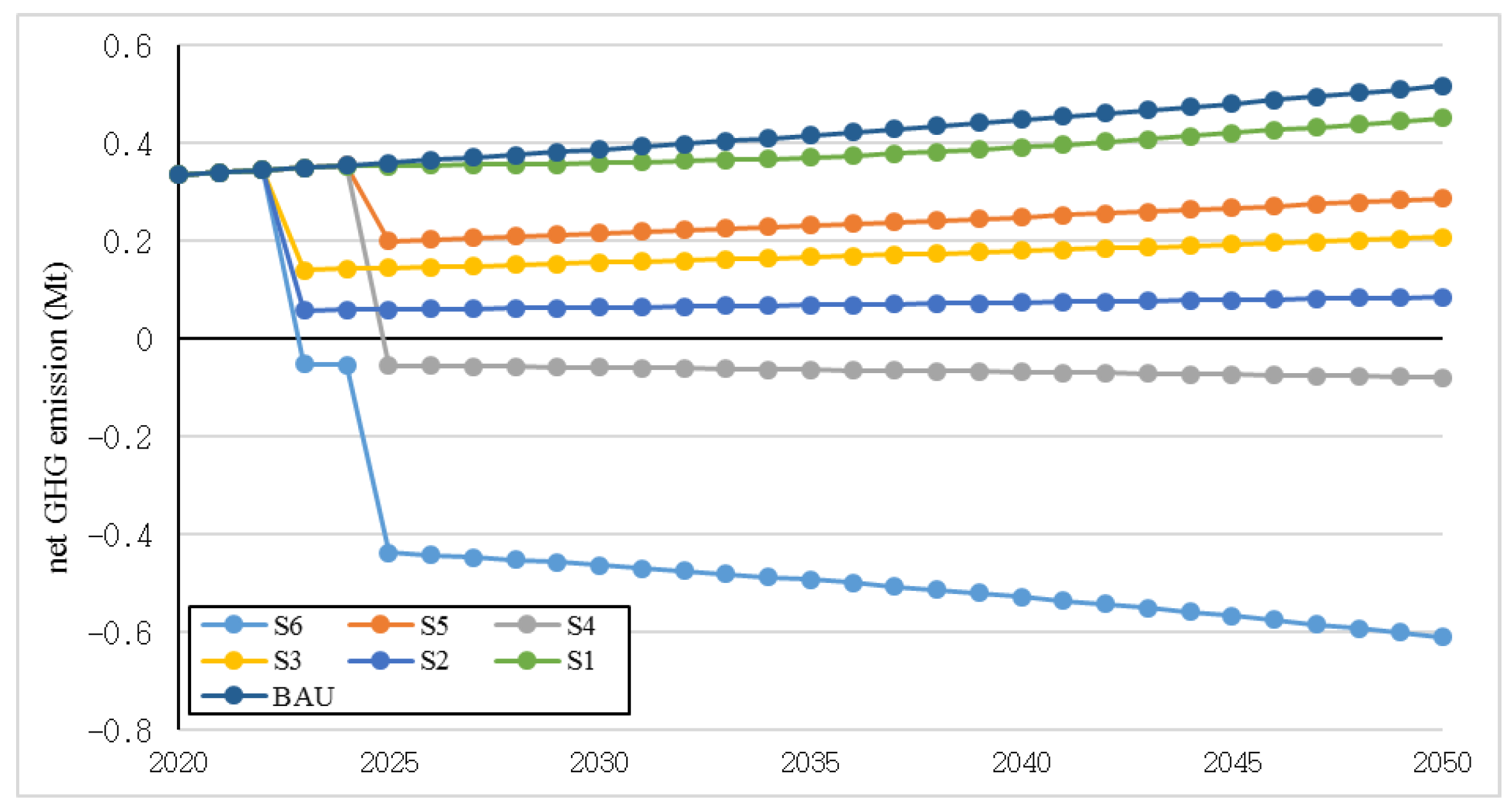
3.3. Cumulative Amount of GHGs under Different Scenarios

The cumulative amount of GHG emissions and avoided GHGs in each scenario over the entire simulation period is shown in

Table 4. Cumulative amount of avoided GHGs and GHG emissions under different scenarios during 2020–2050.

Scenarios	Emission (Mt)		Avoided (Mt)		Accumulated Net GHGs 2020–2050 (Mt)	Accumulated Net GHGs Compared to BAU Scenario (Mt)
	GHGs from Different Treatment	GHGs from Input Material	GHGs from Products	GHGs from Input Material Reduction
S6	9.67	1.716	23.19	0.046	−11.86	24.3 (−195%)
S5	15.18	1.010	8.47	0.017	7.70	4.8 (−38.3)
S4	12.42	0.941	13.26	0.023	0.08	12.4 (−99.3%)
S3	14.13	1.514	10.01	0.023	5.62	6.9 (−55%)
S2	7.91	0.283	5.27	0.010	2.91	9.6 (−76.7)
S1	15.43	0.508	4.55	0.019	11.37	1.1 (−8.9)
BAU	14.59	0.283	2.39	0.010	12.48	0

. The GHG emissions in each scenario are the direct emissions because of the different waste treatment methods and indirect emissions are the result of the input materials used for each process. In the entire simulation period, the highest amount of direct GHG emissions can be seen for Scenario S1 (dry waste recycling), in which the unmanaged landfilling of waste and the failure to implement landfill gas control measures had the most significant contributions to emissions; in addition, the recycling of dry waste can cause GHG emissions [41]. In contrast, the lowest amount of GHG emissions was observed in Scenario S2, with 7.91 Mt for the entire simulation period. The lowest amounts of indirect GHG emissions were observed in the BAU Scenario and Scenario S2, because the energy required for the landfill process is less than the other processes (0.283 Mt for the entire simulation period). At the same time, the highest amount of indirect GHG emissions was observed in Scenario S6 due to the use of different waste treatment methods and consumption of input materials (1.716 Mt for the entire simulation period).

In order to more accurately investigate GHGs, in addition to the amount of GHG emissions, the avoided GHGs through different waste management methods should be considered [80,81]. Avoided GHGs are obtained by reducing transportation and the recovery of materials as a result of recycling (S1), production of fertilizer as a result of composting (S3) and aerobic digestion (S4), and the production of electricity as a result of anaerobic digestion (S4), waste incineration (S5), and sanitary landfilling (S2). Using a combination of all of the treatment methods in Scenario S6, the highest amount of avoided GHGs was 23.19 Mt for the entire simulation period, while the lowest amount of avoided GHGs was 2.39 Mt in the BAU Scenario. Reducing energy consumption by diverting waste from landfills can also lead to avoided GHGs, whose contribution to GHG flow is insignificant, so the highest avoided GHGs in Scenario S6 was 0.046 Mt for the whole period of the simulation.

In general, the cumulative net GHG emissions would reach 12.48 Mt if no management measures were taken into consideration (i.e., BAU Scenario), in which direct GHG emissions from an unmanaged landfill were the main contributions. However, the net accumulated GHG emissions in Scenario S6 become negative after 2028 and reached −11.86 Mt, which is a 195% decrease, and the avoided GHGs had the largest role in the GHG mitigation (Table 4). The recycling of recyclable products from valuable dry waste and the production of products in different treatment methods offset the emission of GHGs produced by burning coal or natural gas. An EPA report found that for each 1 ton of waste treated, this decreases approximately 1 ton of CO₂ emissions [74].

3.4. Damage Assessment through the Endpoint Approach

The amount of damage to safeguard subjects is presented in

Table 5. The amount of damage to the four safeguard subjects under different scenarios.

	Unit	BAU	S1	S2	S3	S4	S5	S6
SA	USD	1.7 × 108	1.5 × 108	1.5 × 108	1.1 × 108	1.5 × 108	1.3 × 108	4.3 × 107
	USD	4.3 × 108	4.0 × 108	4.0 × 108	3.0 × 108	4.0 × 108	3.2 × 108	1.1 E× 108
PP	Kg	2.3 × 108	2.1 × 108	2.1 × 108	1.6 × 108	2.1 × 108	1.7 × 108	5.8 × 107
	USD	1.3 × 107	1.2 × 107	1.2 × 107	8.9 × 106	1.2 × 107	9.5 × 106	3.2 × 106
HH	DALY	5.9 × 103	6.3 × 103	3.1 × 103	5.7 × 103	6.3 × 103	6.2 × 103	3.9 × 103
	USD	1.4 × 108	1.5 × 108	7.5 × 107	1.4 × 108	1.5 × 108	1.5 × 108	9.2 × 107
Net HH	DALY	8.2 × 10−3	7.4 × 10−3	1.7 × 10−3	3.5 × 10−3	7.6 × 10−3	4.9 × 10−3	−8.3 × 10−3
	USD	9.0 × 107	8.2 × 107	1.8 × 107	3.9 × 107	8.4 × 107	5.4 × 107	−9.1 × 107
BD	EINES	9.9 × 10−3	1.0 × 10−2	5.4 × 10−3	9.6 × 10−3	1.1 × 10−2	1.0 × 10−2	6.6 × 10−3
	USD	1.1 × 108	1.2 × 108	5.9 × 107	1.1 × 108	1.2 × 108	1.1 × 108	7.2 × 107
Net BD	EINES	8.2 × 10−3	7.4 × 10−3	1.7 × 10−3	3.5 × 10−3	7.6 × 10−3	4.9 × 10−3	−8.3 × 10−3
	USD	9.0 × 107	8.2 × 108	1.9 × 107	3.9 × 107	8.4 × 107	5.4 × 107	−9.1 × 107

. Damage to human health (in units of DALY) results from GHG emissions. The lowest damage to human health was observed in Scenario S2, at 3.1 × 10³ DALY, which was reduced by 46% compared to the BAU Scenario. While considering the DALY savings, the least damage to human health was in Scenario S6, at −8.3 × 10⁻³ DALY, which is 222% less than in the BAU Scenario. The greatest damage to human health is in Scenario S1, which increased by 6% compared to the BAU Scenario; considering the DALY savings, the damage to human health reduced by 9% compared to the BAU Scenario. Irrespective of the DALY savings, in Alborz Province, the amount of damage to human health for 2.7 million people over a lifespan of 76 years in Scenario S1 was equal to 7.77 × 10⁻⁵ for each person. The DALY savings, especially in Scenarios S4 and S6, were significant enough to offset the human health losses. Therefore, the actual human health damage is represented by considering the DALY savings through the net damage, which represents the negative outcomes and compensates for the damage to human health.

Biodiversity damage, expressed as EINES, results from GHG emissions, waste disposal, and land use. The results show that the most significant damage to biodiversity is in Scenario S1, with 1.6 × 10⁻¹¹ EINES per ton of waste, which is due to the emission of GHGs in the processes of recycling and landfilling waste and from the increasing land use. While in Scenario S2, with the transfer of all wastes to the landfill, the least damage to biodiversity with 5.4 × 10⁻³ EINES was observed, which is due to landfill gas control. Damage to biodiversity is offset by EINES savings; in relation to Scenarios S6 and S4, the net damage to biodiversity was negative, indicating compensation for biodiversity damage. Although the damage to human health and biodiversity in Scenario S2 from the sanitary burial was less than the other processes, considering the damage savings, however, the anaerobic digestion in Scenario S4 had the least damage to human health and biodiversity.

Damage to social assets (in USD units) and primary productivity (in Kg units) is caused by waste landfilling and land use; in the BAU Scenario, the most damage was caused to social assets and primary productivity, while the least damage was observed in Scenario S6. The main reason for the reduction in the damage to social assets and primary productivity in Scenario S6 was the diversion of waste from the landfill to other processes, which led to less land use. The amount of damage to social assets and primary productivity in the BAU Scenario per ton of waste was USD 5.9 and 8.1 Kg, respectively, while in Scenario S6, it is USD 1.5 and 2.1 × 10⁰ Kg, respectively. Despite the deviation of 50% of the organic materials in the landfill in Scenarios S3 and S4, the anaerobic digester process had the least damage to social assets and primary productivity among the different processes due to less residue.

In general, considering that Scenario S6 is the result of the management of all wastes in the different proposed processes, the least damage to safeguard subjects was observed in this scenario. Among the different processes, anaerobic digestion, due to less residual and more damage savings because of the production of electricity and compost production, showed the least damage in terms of safeguard subjects compared to the other processes.

3.5. Damage Cost Assessment through the Endpoint Approach

The arrangement among the safeguard subjects in terms of monetary damage, based on USD, in all of the scenarios was social assets > human health > biodiversity > primary productivity (Table 5). The irrational disposal of waste demolishes a large amount of social resources to reduce its environmental damage [17].

The social assets damage cost in the BAU Scenario in the simulation period was USD 428 million, while in Scenarios S1, S2, S3, S4, S5, and S6 reached USD 401 million, USD 398 million, USD 302 million, USD 291 million, USD 323 million, and USD 109 million with a 6%, 7%, 29%, 32%, 24%, and 74% reduction compared to the BAU Scenario, respectively. The amount of primary productivity damage in the simulation period for the BAU Scenario was USD 12.6 million; in Scenarios S1 and S2, it reached USD 11.8 and 11.7 million with a 6% and 7% decrease compared to the BAU Scenario, respectively. Moreover, damage to the primary productivity in S3, S4, S5, and S6 reached USD 8.9 million, USD 8.6 million, USD 9.5 million, and USD 3.2 million, respectively (Table 5).

In connection with the two other issues, human health and biodiversity, taking into account the damage savings, the net damage was obtained through the difference between the damage and damage savings. Unlike social assets and primary productivity, the lowest human health and biodiversity damage cost was in Scenario S2, which were USD 75 million and USD 59 million, respectively. However, considering the damage cost savings, the lowest amount of net human health and biodiversity damage cost were observed in Scenario S6, and the net amount of damage to human health, taking into account the USD 92 million damage cost and USD 184 million damage cost savings, reached USD −91 million. In addition, the net amount of damage to the biodiversity also reached USD −91 million, taking into account the USD 72 million damage cost and the USD 163 million damage cost savings (Table 5).

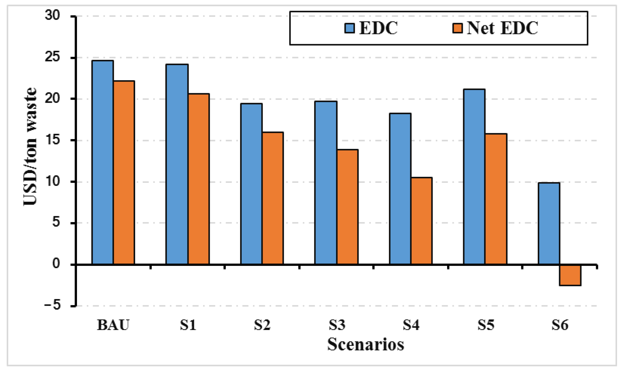
3.6. Environmental Damage Cost

According to the amount of landfilled waste and GHG emissions in each scenario, the environmental damage cost was determined based on the LIME model [17]. In addition, in this study, taking into account the emission and avoided GHGs from the input materials and the production of products in different scenarios, the net environmental damage cost was determined and is presented in Figure 5.

The BAU Scenario had the highest environmental damage cost, with USD 689 million for the simulation period, and with only USD 69 million in environmental damage cost savings, the net environmental damage cost in this scenario was USD 620 million. The total environmental damage cost under Scenario S1 (after the separation of valuable dry waste) in the simulation period was USD 676 million, which is only 1.9% less than the BAU Scenario (without waste separation). This indicates that waste separation did not have a significant effect on the environmental damage cost reduction. Considering the environmental damage cost savings in this scenario, which was USD 99 million, the net environmental damage cost for the entire simulation period was USD 576 million. Landfill gas recovery in the sanitary landfill, in addition to the lower environmental damage cost, led to environmental damage cost savings through the production of electricity in the landfill, so the net environmental damage cost compared to the BAU Scenario decreased by 27.9% to USD 447 million. Scenarios S3 and S4 can further reduce the environmental damage cost by USD 137 and 178 million, respectively, demonstrating the advantage of anaerobic digestion over composting in reducing the environmental damage cost due to lower amounts of GHG emissions and residuals. In addition, because of the use of electricity and production of compost, the amount of environmental damage cost savings in Scenario S4 at the end of the simulation period was USD 217.1 million, with a 33% increase compared to Scenario S3. The net environmental damage cost was USD 388 million in Scenario S3 and USD 294 million in Scenario S4, which decreased compared to the BAU Scenario by 37% and 53%, respectively. The total environmental damage cost in Scenario S5 decreased by USD 98 million compared to the BAU Scenario and reached USD 591 million. Considering the environmental damage cost savings of USD 150 million due to electricity production with the incinerator, the net environmental damage cost for the entire simulation period was USD 441 million, which is a decrease of 29% compared to the BAU Scenario.

With the implementation of ISWM in Scenario S6, on the one hand, the environmental damage cost increased to a lower slope and by the end of the simulation period it had reached USD 277 million. On the other hand, the amount of environmental damage cost savings due to the exploitation of electrical energy and compost production from the various processes increased and reached USD 347 million, so the net environmental damage cost was USD −71 million at the end of the simulation period. As can be seen in Figure 5, the net environmental damage cost had been less than zero since 2038 with the increase in the environmental damage cost savings compared to the environmental damage cost. As shown in Figure 6, the environmental damage cost per ton of waste in the BAU Scenario was USD 24.6, which considered the environmental damage cost savings, and the net environmental damage cost was 22.2 USD/ton, while the environmental damage cost in Scenario S6 was 10 USD/ton, and by taking into account the environmental damage cost savings, the net environmental damage cost per ton of waste in this scenario was USD −2.5. In general, Scenario S6 not only had no environmental costs but also had environmental damage cost savings.

In an integrated system, first, the valuable dry wastes are separated for recycling at the source, organic materials enter the mechanical biological treatment process (composting and anaerobic digestion), and then the remaining dry wastes that have a high calorific value enter the waste incinerator to produce energy. Finally, the residuals of the waste and treatment processes enter the sanitary landfill [75,82]. The use of the advantages of each waste management method, as obtained in Scenarios S1 to S5, is the reason for the better performance of Scenario S6. In the EU, the gradual transition from MSW management based on landfilling to integrated management based on the optimum use of existing technologies (i.e., composting, anaerobic digestion, recycling, incineration with energy recovery, and landfilling) has caused a reduction in GHG emissions, as well as the avoidance of emissions. Therefore, the emissions due to this waste management system are close to or already a carbon sink [78].

3.7. Contribution of Safeguard Subjects to EDC

The contribution of the safeguard subjects to the environmental damage cost is shown in Figure 7. Social assets had the greatest effect on the environmental damage cost in all of the scenarios; this was due to the transfer of waste to the landfill either directly or as a residual of the processes. In addition, by considering the damage savings, the contribution of human health and biodiversity damage decreased while the contribution of social assets damage increased.

The contribution of social assets in Scenarios BAU, S1, and S2 was greater than in the other scenarios, with the difference being that in Scenario S2 (i.e., sanitary landfill), by reducing the contribution of the damage to human health and biodiversity through landfill gas control, the contribution of social assets damage increased. The contributions of social assets, human health, biodiversity, and primary productivity in Scenario S2 were 73%, 14%, 11%, and 2%, respectively (Figure 7a); by calculating the damage savings, the contribution of human health and biodiversity was reduced to 4%, and the contribution of social assets increased to 89% (Figure 7b).

In Scenarios S3, S4, and S5, on the one hand, the contribution of social assets decreased with the diversion of waste from the landfill. On the other hand, in terms of GHG emissions, through the processes of composting, anaerobic digestion, and incineration, this led to a reduction in the share of social assets and an increase in the share of human health and biodiversity. Considering the damage savings, the share of human health and biodiversity will decrease drastically; instead, the contribution of social assets will increase. Therefore, the contribution of social assets in Scenario S4 was 99%, and the contribution of human health and biodiversity was 1% in the calculation for the net environmental damage cost.

In Scenario S6, only the residual waste of the various methods was transferred to the landfill. Accordingly, the contribution of the social assets damage was less than in the other scenarios. In addition, the contribution of human health and biodiversity damage increased because of the GHG emissions in the different processes (Figure 7a). However, taking into account the savings damage, the net environmental damage cost was USD −91 million, for which human health and biodiversity played the main role in the environmental damage cost savings (Figure 7b).

4. Conclusions

Waste management planning requires a comprehensive model to analyze possible scenarios for choosing an appropriate solution with the minimum environmental impact and maximum resource recovery. An accurate estimation of the environmental damage cost is possible through the emission inventory of different methods along with the avoided effects caused by waste-based products. Life cycle assessment methods have been widely used as a tool to estimate the environmental performance of waste management systems. The life cycle assessment method helps decision-makers choose the best option by quantifying the impacts of different waste treatment options. The SD approach is suggested as a suitable tool for waste flow modeling; accordingly, this approach was used in order to create a comprehensive model to evaluate the life cycle of different waste scenarios in this study.

The results show that under the BAU Scenario during 2020–2050, the volume of waste accumulated in the landfill reached over 58.5 Mm³, six times higher than the remaining capacity of the landfill center, and the accumulated net GHG emissions reached 12.5 Mt. However, with the simultaneous implementation of the recycling, composting, anaerobic digestion, and incineration programs (Scenario S6), the least volume of landfilled waste was observed, which indicates a 73% decrement compared to the BAU Scenario; in addition, the highest mitigation potential of the net accumulated GHGs was observed, which indicates a 195% reduction compared to the BAU Scenario in the simulation period.

The most damage related to SA, NPP, BD, and HH, as well as the highest environmental damage cost, was observed in the BAU Scenario because of the transfer of all wastes to the landfill. With the implementation of integrated waste management in Scenario S6, on the one hand, the environmental damage cost decreased compared to the BAU Scenario, and it reached USD 277 million. On the other hand, the amount of EDC savings increased to USD 347 million, so the net EDC became negative from 2038 onwards and was USD −71 million at the end of the simulation period.

It can be concluded that considering the avoided emissions using different treatment methods shows a more accurate estimate of the environmental damage cost. In addition, a beneficial integrated solid waste management system for all waste components generates a win–win status in which waste management is accompanied by social benefits (providing advantages to people, employment of a significant number of people, and reducing health risks), environmental benefits (preventing local pollution, conserving a significant amount of resources, and maximizing environmental protection), and economic benefits (generating income for local authorities and stakeholders in the recycling process chain) [83,84]. These further advantages of waste management are commonly called co-advantages [77]. From the results, it is proposed that waste management policies that focus on integrated waste management by strengthening waste segregation and using biological treatment methods, incineration, and sanitary landfills are likely to be more sustainable and, ultimately, achieve the goal of a circular economy by increasing material recovery. The SD modeling approach can be applied by providing an overview of the waste management system and testing different policies and strategies for sustainable waste management. In addition, it is possible to develop the model by adding new instruments, variables, and policy elements.

References

1. Rodić, L.; Wilson, D.C. Resolving Governance Issues to Achieve Priority Sustainable Development Goals Related to Solid Waste Management in Developing Countries. Sustainability 2017, 9, 404. [Google Scholar] [CrossRef]
2. Sadeghi Ahangar, S.; Sadati, A.; Rabbani, M. Sustainable design of a municipal solid waste management system in an integrated closed-loop supply chain network using a fuzzy approach: A case study. J. Ind. Prod. Eng. 2021, 38, 323–340. [Google Scholar] [CrossRef]
3. Browning, S.; Beymer-Farris, B.; Seay, J.R. Addressing the challenges associated with plastic waste disposal and management in developing countries. Curr. Opin. Chem. Eng. 2021, 32, 100682. [Google Scholar] [CrossRef]
4. Patwa, N.; Sivarajah, U.; Seetharaman, A.; Sarkar, S.; Maiti, K.; Hingorani, K. Towards a circular economy: An emerging economies context. J. Bus. Res. 2021, 122, 725–735. [Google Scholar] [CrossRef]
5. Siddiqi, A.; Haraguchi, M.; Narayanamurti, V. Urban waste to energy recovery assessment simulations for developing countries. World Dev. 2020, 131, 104949. [Google Scholar] [CrossRef]
6. Maiurova, A.; Kurniawan, T.A.; Kustikova, M.; Bykovskaia, E.; Othman, M.H.D.; Singh, D.; Goh, H.H. Promoting digital transformation in waste collection service and waste recycling in Moscow (Russia): Applying a circular economy paradigm to mitigate climate change impacts on the environment. J. Clean. Prod. 2022, 354, 131604. [Google Scholar] [CrossRef]
7. Song, J.; Feng, R.; Yue, C.; Shao, Y.; Han, J.; Xing, J.; Yang, W. Reinforced urban waste management for resource, energy and environmental benefits: China’s regional potentials. Resour. Conserv. Recycl. 2022, 178, 106083. [Google Scholar] [CrossRef]
8. Moeinaddini, M.; Khorasani, N.; Danehkar, A.; Darvishsefat, A.A.; Zienalyan, M. Siting MSW landfill using weighted linear combination and analytical hierarchy process (AHP) methodology in GIS environment (case study: Karaj). Waste Manag. 2010, 30, 912–920. [Google Scholar] [CrossRef]
9. González Martínez, T.; Bräutigam, K.-R.; Seifert, H. The potential of a sustainable municipal waste management system for Santiago de Chile, including energy production from waste. Energy Sustain. Soc. 2012, 2, 24. [Google Scholar] [CrossRef]
10. Tsai, F.M.; Bui, T.-D.; Tseng, M.-L.; Lim, M.K.; Hu, J. Municipal solid waste management in a circular economy: A data-driven bibliometric analysis. J. Clean. Prod. 2020, 275, 124132. [Google Scholar] [CrossRef]
11. Liao, N.; Bolyard, S.C.; Lü, F.; Yang, N.; Zhang, H.; Shao, L.; He, P. Can waste management system be a Greenhouse Gas sink? Perspective from Shanghai, China. Resour. Conserv. Recycl. 2022, 180, 106170. [Google Scholar] [CrossRef]
12. Zhang, C.; Dong, H.; Geng, Y.; Song, X.; Zhang, T.; Zhuang, M. Carbon neutrality prediction of municipal solid waste treatment sector under the shared socioeconomic pathways. Resour. Conserv. Recycl. 2022, 186, 106528. [Google Scholar] [CrossRef]
13. Christensen, T.H.; Damgaard, A.; Levis, J.; Zhao, Y.; Björklund, A.; Arena, U.; Barlaz, M.A.; Starostina, V.; Boldrin, A.; Astrup, T.F.; et al. Application of LCA modelling in integrated waste management. Waste Manag. 2020, 118, 313–322. [Google Scholar] [CrossRef] [PubMed]
14. Khandelwal, H.; Dhar, H.; Thalla, A.K.; Kumar, S. Application of life cycle assessment in municipal solid waste management: A worldwide critical review. J. Clean. Prod. 2019, 209, 630–654. [Google Scholar] [CrossRef]
15. Dijkgraaf, E.; Vollebergh, H.R.J. Burn or bury? A social cost comparison of final waste disposal methods. Ecol. Econ. 2004, 50, 233–247. [Google Scholar] [CrossRef]
16. Yi, S.; Kurisu, K.H.; Hanaki, K. Life cycle impact assessment and interpretation of municipal solid waste management scenarios based on the midpoint and endpoint approaches. Int. J. Life Cycle Assess. 2011, 16, 652–668. [Google Scholar] [CrossRef]
17. Liu, C.; Dong, H.; Cao, Y.; Geng, Y.; Li, H.; Zhang, C.; Xiao, S. Environmental damage cost assessment from municipal solid waste treatment based on LIME3 model. Waste Manag. 2021, 125, 249–256. [Google Scholar] [CrossRef]
18. Ooi, J.K.; Woon, K.S.; Hashim, H. A multi-objective model to optimize country-scale municipal solid waste management with economic and environmental objectives: A case study in Malaysia. J. Clean. Prod. 2021, 316, 128366. [Google Scholar] [CrossRef]
19. Amaral, R.E.C.; Brito, J.; Buckman, M.; Drake, E.; Ilatova, E.; Rice, P.; Sabbagh, C.; Voronkin, S.; Abraham, Y.S. Waste Management and Operational Energy for Sustainable Buildings: A Review. Sustainability 2020, 12, 5337. [Google Scholar] [CrossRef]
20. Rajaeifar, M.A.; Ghanavati, H.; Dashti, B.B.; Heijungs, R.; Aghbashlo, M.; Tabatabaei, M. Electricity generation and GHG emission reduction potentials through different municipal solid waste management technologies: A comparative review. Renew. Sustain. Energy Rev. 2017, 79, 414–439. [Google Scholar] [CrossRef]
21. Sauve, G.; Van Acker, K. The environmental impacts of municipal solid waste landfills in Europe: A life cycle assessment of proper reference cases to support decision making. J. Environ. Manag. 2020, 261, 110216. [Google Scholar] [CrossRef] [PubMed]
22. Yao, X.; Guo, Z.; Liu, Y.; Li, J.; Feng, W.; Lei, H.; Gao, Y. Reduction potential of GHG emissions from municipal solid waste incineration for power generation in Beijing. J. Clean. Prod. 2019, 241, 118283. [Google Scholar] [CrossRef]
23. Lu, H.R.; Qu, X.; El Hanandeh, A. Towards a better environment—The municipal organic waste management in Brisbane: Environmental life cycle and cost perspective. J. Clean. Prod. 2020, 258, 120756. [Google Scholar] [CrossRef]
24. Nevrlý, V.; Šomplák, R.; Putna, O.; Pavlas, M. Location of mixed municipal waste treatment facilities: Cost of reducing greenhouse gas emissions. J. Clean. Prod. 2019, 239, 118003. [Google Scholar] [CrossRef]
25. Salmeron, J.L.; Vidal, R.; Mena, A. Ranking fuzzy cognitive map based scenarios with TOPSIS. Expert Syst. Appl. 2012, 39, 2443–2450. [Google Scholar] [CrossRef]
26. Kollikkathara, N.; Feng, H.; Yu, D. A system dynamic modeling approach for evaluating municipal solid waste generation, landfill capacity and related cost management issues. Waste Manag. 2010, 30, 2194–2203. [Google Scholar] [CrossRef]
27. Babalola, M.A. A System Dynamics-Based Approach to Help Understand the Role of Food and Biodegradable Waste Management in Respect of Municipal Waste Management Systems. Sustainability 2019, 11, 3456. [Google Scholar] [CrossRef]
28. Sukholthaman, P.; Sharp, A. A system dynamics model to evaluate effects of source separation of municipal solid waste management: A case of Bangkok, Thailand. Waste Manag. 2016, 52, 50–61. [Google Scholar] [CrossRef]
29. Di Nola, M.F.; Escapa, M.; Ansah, J.P. Modelling solid waste management solutions: The case of Campania, Italy. Waste Manag. 2018, 78, 717–729. [Google Scholar] [CrossRef]
30. Lee, C.K.M.; Ng, K.K.H.; Kwong, C.K.; Tay, S.T. A system dynamics model for evaluating food waste management in Hong Kong, China. J. Mater. Cycles Waste Manag. 2019, 21, 433–456. [Google Scholar] [CrossRef]
31. Xiao, S.; Dong, H.; Geng, Y.; Tian, X.; Liu, C.; Li, H. Policy impacts on Municipal Solid Waste management in Shanghai: A system dynamics model analysis. J. Clean. Prod. 2020, 262, 121366. [Google Scholar] [CrossRef]
32. Dyson, B.; Chang, N.-B. Forecasting municipal solid waste generation in a fast-growing urban region with system dynamics modeling. Waste Manag. 2005, 25, 669–679. [Google Scholar] [CrossRef] [PubMed]
33. Estay-Ossandon, C.; Mena-Nieto, A. Modelling the driving forces of the municipal solid waste generation in touristic islands. A case study of the Balearic Islands (2000–2030). Waste Manag. 2018, 75, 70–81. [Google Scholar] [CrossRef] [PubMed]
34. Dianati, K.; Schäfer, L.; Milner, J.; Gómez-Sanabria, A.; Gitau, H.; Hale, J.; Langmaack, H.; Kiesewetter, G.; Muindi, K.; Mberu, B.; et al. A system dynamics-based scenario analysis of residential solid waste management in Kisumu, Kenya. Sci. Total Environ. 2021, 777, 146200. [Google Scholar] [CrossRef]
35. Wang, W.-J.; You, X.-Y. Benefits analysis of classification of municipal solid waste based on system dynamics. J. Clean. Prod. 2021, 279, 123686. [Google Scholar] [CrossRef]
36. Xiao, S.; Dong, H.; Geng, Y.; Tian, X. Low carbon potential of urban symbiosis under different municipal solid waste sorting modes based on a system dynamic method. Resour. Conserv. Recycl. 2022, 179, 106108. [Google Scholar] [CrossRef]
37. Hosseinalizadeh, R.; Shakouri, G.H.; Izadbakhsh, H. Planning for energy production from municipal solid waste: An optimal technology mix via a hybrid closed-loop system dynamics-optimization approach. Expert Syst. Appl. 2022, 199, 116929. [Google Scholar] [CrossRef]
38. Sterman, J. System Dynamics: Systems Thinking and Modeling for a Complex World; MIT Sloan School of Management: Cambridge, MA, USA, 2002. [Google Scholar]
39. Hu, W.; Camacho, E.F.; Xie, L. Feedforward and feedback control of dynamic systems. IFAC Proc. Vol. 2014, 47, 7741–7748. [Google Scholar] [CrossRef]
40. Amjad, J. Effectiveness Assessment of Air Pollution Reduction Plans in Karaj Waste Collection System Based on Life Cycle Prespective. Master’s Thesis, Department of Environment, Faculty of Natural Resources, College of Agriculture and Natural Resources, University of Tehran, Tehran, Iran, 2021. [Google Scholar]
41. Tsewng, C.-H.; Hsu, Y.-C.; Chen, Y.-C. System dynamics modeling of waste management, greenhouse gas emissions, and environmental costs from convenience stores. J. Clean. Prod. 2019, 239, 118006. [Google Scholar] [CrossRef]
42. Yang, N.; Li, F.; Liu, Y.; Dai, T.; Wang, Q.; Zhang, J.; Dai, Z.; Yu, B. Environmental and Economic Life-Cycle Assessments of Household Food Waste Management Systems: A Comparative Review of Methodology and Research Progress. Sustainability 2022, 14, 7533. [Google Scholar] [CrossRef]
43. Eggleston, H.S.; Buendia, L.; Miwa, K.; Ngara, T.; Tanabe, K. (Eds.) IPCC Guidelines for National Greenhouse Gas Inventories; Prepared by the National Greenhouse Gas Inventories Programme; IGES: Hayama, Japan, 2006. [Google Scholar]
44. Fertilizers Europe. Average Emissions Year 2014. Fertilizers Europe Environmental Report (Internal). Used for Updated Energy and GHG Emission in Carbon Footprint Calculator; Fertilizers Europe: Tehran, Iran, 2006. [Google Scholar]
45. Rashid, M.I.; Shahzad, K. Food waste recycling for compost production and its economic and environmental assessment as circular economy indicators of solid waste management. J. Clean. Prod. 2021, 317, 128467. [Google Scholar] [CrossRef]
46. Ayodele, T.R.; Ogunjuyigbe, A.S.O.; Alao, M.A. Economic and environmental assessment of electricity generation using biogas from organic fraction of municipal solid waste for the city of Ibadan, Nigeria. J. Clean. Prod. 2018, 203, 718–735. [Google Scholar] [CrossRef]
47. Hosseinalizadeh, R.; Izadbakhsh, H.; Shakouri, G.H. A planning model for using municipal solid waste management technologies- considering Energy, Economic, and Environmental Impacts in Tehran-Iran. Sustain. Cities Soc. 2021, 65, 102566. [Google Scholar] [CrossRef]
48. Haupt, M.; Kagi, T.; Hellweg, S. Life cycle inventories of waste management processes. Data Brief 2018, 19, 1441–1457. [Google Scholar] [CrossRef]
49. Cadena, E.; Colón, J.; Artola, A.; Sánchez, A.; Font, X. Environmental impact of two aerobic composting technologies using life cycle assessment. Int. J. Life Cycle Assess. 2009, 14, 401–410. [Google Scholar] [CrossRef]
50. Opatokun, S.A.; Lopez-Sabiron, A.; Ferreira, G.; Strezov, V. Life Cycle Analysis of Energy Production from Food Waste through Anaerobic Digestion, Pyrolysis and Integrated Energy System. Sustainability 2017, 9, 1804. [Google Scholar] [CrossRef]
51. Damgaard, A.; Riber, C.; Fruergaard, T.; Hulgaard, T.; Christensen, T.H. Life-cycle-assessment of the historical development of air pollution control and energy recovery in waste incineration. Waste Manag. 2010, 30, 1244–1250. [Google Scholar] [CrossRef]
52. Hong, J.; Li, X.; Zhaojie, C. Life cycle assessment of four municipal solid waste management scenarios in China. Waste Manag. 2010, 30, 2362–2369. [Google Scholar] [CrossRef]
53. PRI. Compilation of Pollution Atlas of Power Plants in the Country; Power Research Institute: Tehran, Iran, 2008. (In Persion) [Google Scholar]
54. McDougall, F.R.; White, P.R.; Franke, M.; Hindle, P. Integrated Solid Waste Management: A Life Cycle Inventory; John Wiley & Sons: Hoboken, NJ, USA, 2008. [Google Scholar]
55. Haight, M. Integrated Solid Waste Management Model; Technical Report; University of Waterloo, School of Planning: Waterloo, ON, Canada, 2004. [Google Scholar]
56. Itsubo, N.; Inaba, A. A new LCIA method: LIME has been completed. Int. J. Life Cycle Assess. 2003, 8, 305. [Google Scholar] [CrossRef]
57. Itsubo, N.; Inaba, A. LIME2 Life-Cycle Impact Assessment Method Based on Endpoint Modeling; Life-Cycle Assessment Society of Japan: Tokyo, Japan, 2012. [Google Scholar]
58. Itsubo, N.; Murakami, K.; Kuriyama, K.; Yoshida, K.; Tokimatsu, K.; Inaba, A. Development of weighting factors for G20 countries—Explore the difference in environmental awareness between developed and emerging countries. Int. J. Life Cycle Assess. 2018, 23, 2311–2326. [Google Scholar] [CrossRef]
59. Matsuno, Y.; Itsubo, N.; Hondo, H.; Nakano, K. LCA in Japan in the twenty-first century. Int. J. Life Cycle Assess. 2013, 18, 278–284. [Google Scholar] [CrossRef]
60. Mak, T.M.W.; Chen, P.-C.; Wang, L.; Tsang, D.C.W.; Hsu, S.C.; Poon, C.S. A system dynamics approach to determine construction waste disposal charge in Hong Kong. J. Clean. Prod. 2019, 241, 118309. [Google Scholar] [CrossRef]
61. Sinha, R.; Laurenti, R.; Singh, J.; Malmström, M.E.; Frostell, B. Identifying ways of closing the metal flow loop in the global mobile phone product system: A system dynamics modeling approach. Resour. Conserv. Recycl. 2016, 113, 65–76. [Google Scholar] [CrossRef]
62. Qudrat-Ullah, H.; Seong, B.S. How to do structural validity of a system dynamics type simulation model: The case of an energy policy model. Energy Policy 2010, 38, 2216–2224. [Google Scholar] [CrossRef]
63. Robalino-López, A.; Mena-Nieto, Á.; García-Ramos, J.-E.; Golpe, A.A. Studying the relationship between economic growth, CO2 emissions, and the environmental Kuznets curve in Venezuela (1980–2025). Renew. Sustain. Energy Rev. 2015, 41, 602–614. [Google Scholar] [CrossRef]
64. Lewis, C.D. Industrial and Business Forecasting Methods: A Practical Guide to Exponential Smoothing and Curve Fitting; Butterworth Scientific London: London, UK, 1982. [Google Scholar]
65. Zuberi, M.J.S.; Ali, S.F. Greenhouse effect reduction by recovering energy from waste landfills in Pakistan. Renew. Sustain. Energy Rev. 2015, 44, 117–131. [Google Scholar] [CrossRef]
66. Lino, F.A.M.; Ismail, K.A.R. Evaluation of the treatment of municipal solid waste as renewable energy resource in Campinas, Brazil. Sustain. Energy Technol. Assess. 2018, 29, 19–25. [Google Scholar] [CrossRef]
67. Abdelaal, A.H.; McKay, G.; Mackey, H.R. Food waste from a university campus in the Middle East: Drivers, composition, and resource recovery potential. Waste Manag. 2019, 98, 14–20. [Google Scholar] [CrossRef]
68. Rafiee, R. Conducting Studies and Presenting an Operational Plan for Standardization and Improvement of Waste Processing and Disposal Processes and Leachate Management in Halghedareh; Department of Environment, Faculty of Natural Resources, College of Agriculture and Natural Resources, University of Tehran: Tehran, Iran, 2020. [Google Scholar]
69. Bogner, J.; Pipatti, R.; Hashimoto, S.; Diaz, C.; Mareckova, K.; Diaz, L.; Kjeldsen, P.; Monni, S.; Faaij, A.; Gao, Q.; et al. Mitigation of global greenhouse gas emissions from waste: Conclusions and strategies from the Intergovernmental Panel on Climate Change (IPCC) Fourth Assessment Report. Working Group III (Mitigation). Waste Manag. Res. 2008, 26, 11–32. [Google Scholar] [CrossRef]
70. Di Trapani, D.; Di Bella, G.; Viviani, G. Uncontrolled methane emissions from a MSW landfill surface: Influence of landfill features and side slopes. Waste Manag. 2013, 33, 2108–2115. [Google Scholar] [CrossRef]
71. Moghadam, M.A.; Feizi, R.; Panahi Fard, M.; Haghighi Fard, N.J.; Omidinasab, M.; Faraji, M.; Shenavar, B. Estimating greenhouse emissions from sanitary landfills using Land-GEM and IPCC model based on realistic scenarios of different urban areas: A case study of Iran. J. Environ. Health Sci. Eng. 2021, 19, 819–830. [Google Scholar] [CrossRef] [PubMed]
72. Calabrò, P.S. Greenhouse gases emission from municipal waste management: The role of separate collection. Waste Manag. 2009, 29, 2178–2187. [Google Scholar] [CrossRef] [PubMed]
73. Weitz, K.A.; Thorneloe, S.A.; Nishtala, S.R.; Yarkosky, S.; Zannes, M. The Impact of Municipal Solid Waste Management on Greenhouse Gas Emissions in the United States. J. Air Waste Manag. Assoc. 2002, 52, 1000–1011. [Google Scholar] [CrossRef] [PubMed]
74. Rena; Arya, S.; Chavan, D.; Aiman, S.; Kumar, S. Reducing Greenhouse Gas Emission From Waste Landfill. In Encyclopedia of Renewable and Sustainable Materials; Hashmi, S., Choudhury, I.A., Eds.; Elsevier: Oxford, UK, 2020; pp. 685–701. [Google Scholar] [CrossRef]
75. Liu, Y.; Ni, Z.; Kong, X.; Liu, J. Greenhouse gas emissions from municipal solid waste with a high organic fraction under different management scenarios. J. Clean. Prod. 2017, 147, 451–457. [Google Scholar] [CrossRef]
76. Hansen, T.L.; Bhander, G.S.; Christensen, T.H.; Bruun, S.; Jensen, L.S. Life cycle modelling of environmental impacts of application of processed organic municipal solid waste on agricultural land (EASEWASTE). Waste Manag Res 2006, 24, 153–166. [Google Scholar] [CrossRef]
77. Menikpura, S.N.M.; Sang-Arun, J.; Bengtsson, M. Integrated Solid Waste Management: An approach for enhancing climate co-benefits through resource recovery. J. Clean. Prod. 2013, 58, 34–42. [Google Scholar] [CrossRef]
78. Calabrò, P.S.; Gori, M.; Lubello, C. European trends in greenhouse gases emissions from integrated solid waste management. Environ. Technol. 2015, 36, 2125–2137. [Google Scholar] [CrossRef]
79. Panepinto, D.; Genon, G. Carbon dioxide balance and cost analysis for different scenarios of solid waste management. WIT Trans. Ecol. Environ. 2011, 144, 445–456. [Google Scholar]
80. Gentil, E.; Christensen, T.H.; Aoustin, E. Greenhouse gas accounting and waste management. Waste Manag. Res. 2009, 27, 696–706. [Google Scholar] [CrossRef]
81. Tabata, T.; Hishinuma, T.; Ihara, T.; Genchi, Y. Life cycle assessment of integrated municipal solid waste management systems, taking account of climate change and landfill shortage trade-off problems. Waste Manag. Res 2011, 29, 423–432. [Google Scholar] [CrossRef]
82. Wang, K.; Nakakubo, T. Comparative assessment of waste disposal systems and technologies with regard to greenhouse gas emissions: A case study of municipal solid waste treatment options in China. J. Clean. Prod. 2020, 260, 120827. [Google Scholar] [CrossRef]
83. Koroneos, C.J.; Nanaki, E.A. Integrated solid waste management and energy production—A life cycle assessment approach: The case study of the city of Thessaloniki. J. Clean. Prod. 2012, 27, 141–150. [Google Scholar] [CrossRef]
84. Menikpura, S.N.; Gheewala, S.H.; Bonnet, S. Framework for life cycle sustainability assessment of municipal solid waste management systems with an application to a case study in Thailand. Waste Manag. Res. 2012, 30, 708–719. [Google Scholar] [CrossRef]
85. SYAP. Statistical Yearbook of Alborz Province, Program and Budget Organization; SYAP: Alborz, Iran, 2011. [Google Scholar]
86. SYAP. Statistical Yearbook of Alborz Province, Program and Budget Organization; SYAP: Alborz, Iran, 2012. [Google Scholar]
87. SYAP. Statistical Yearbook of Alborz Province, Program and Budget Organization; SYAP: Alborz, Iran, 2013. [Google Scholar]
88. SYAP. Statistical Yearbook of Alborz Province, Program and Budget Organization; SYAP: Alborz, Iran, 2014. [Google Scholar]
89. SYAP. Statistical Yearbook of Alborz Province, Program and Budget Organization; SYAP: Alborz, Iran, 2015. [Google Scholar]
90. SYAP. Statistical Yearbook of Alborz Province, Program and Budget Organization; SYAP: Alborz, Iran, 2016. [Google Scholar]
91. SYAP. Statistical Yearbook of Alborz Province, Program and Budget Organization; SYAP: Alborz, Iran, 2017. [Google Scholar]
92. SYAP. Statistical Yearbook of Alborz Province, Program and Budget Organization; SYAP: Alborz, Iran, 2018. [Google Scholar]
93. SYAP. Statistical Yearbook of Alborz Province, Program and Budget Organization; SYAP: Alborz, Iran, 2019. [Google Scholar]
94. SYAP. Statistical Yearbook of Alborz Province, Program and Budget Organization; SYAP: Alborz, Iran, 2020. [Google Scholar]
95. SYAP. Statistical Yearbook of Alborz Province, Program and Budget Organization; SYAP: Alborz, Iran, 2021. [Google Scholar]
96. SYAP. Statistical Yearbook of Alborz Province, Program and Budget Organization; SYAP: Alborz, Iran, 2022. [Google Scholar]
97. WNA. World Nuclear Association, Carbon Dioxide Emissions From Electricity. Available online: https://www.world-nuclear.org/information-library/energy-and-the-environment/carbon-dioxide-emissions-from-electricity.aspx (accessed on 1 January 2022).
98. Fernández-González, J.M.; Grindlay, A.L.; Serrano-Bernardo, F.; Rodríguez-Rojas, M.I.; Zamorano, M. Economic and environmental review of Waste-to-Energy systems for municipal solid waste management in medium and small municipalities. Waste Manag. 2017, 67, 360–374. [Google Scholar] [CrossRef]
99. IPCC. IPCC Fifth Assessment Report—Synthesis Report; IPCC: New York, NY, USA, 2014. [Google Scholar]
100. TWMO. Waste Production in Tehran; Tehran Waste Management Organization: Tehran, Iran, 2019. [Google Scholar]
101. Worrell, W.A.; Vesilind, P.A.J. Solid Waste Engineering; CL Engineering: Chonburi, Thailand, 2012. [Google Scholar]
102. Ayodele, T.R.; Ogunjuyigbe, A.S.O.; Alao, M.A. Life cycle assessment of waste-to-energy (WtE) technologies for electricity generation using municipal solid waste in Nigeria. Appl. Energy 2017, 201, 200–218. [Google Scholar] [CrossRef]
103. KWMO. Waste Production in Alborz; Karaj Waste Management Organization: Alborz, Iran, 2020. [Google Scholar]
104. Kamarehie, B.; Jafari, A.; Ghaderpoori, M.; Azimi, F.; Faridan, M.; Sharafi, K.; Ahmadi, F.; Karami, M.A. Qualitative and quantitative analysis of municipal solid waste in Iran for implementation of best waste management practice: A systematic review and meta-analysis. Environ. Sci. Pollut. Res. 2020, 27, 37514–37526. [Google Scholar] [CrossRef]
105. Rahmandad, H.; Sterman, J.D. Reporting guidelines for simulation-based research in social sciences. Syst. Dyn. Rev. 2012, 28, 396–411. [Google Scholar] [CrossRef]
Figure 1. Conceptual system dynamics model of a waste stream for different processes.
Sustainability 15 16158 g001
Figure 2. The predicted amount (a) and cumulative volume (b) of waste landfilling under different scenarios.
Sustainability 15 16158 g002
Figure 3. Amount of net GHG emissions in different scenarios during the simulation period.
Sustainability 15 16158 g003
Figure 4. Contributions of the different treatments to net GHG emissions in Scenario S6.
Sustainability 15 16158 g004
Figure 5. Cumulative amount of EDC, EDC savings, and net EDC in different scenarios.
Sustainability 15 16158 g005
Figure 6. The amount of EDC and net EDC in different scenarios per ton waste.
Sustainability 15 16158 g006
Figure 7. The contribution of each of the safeguard subjects: (a) EDC; (b) net EDC.
Sustainability 15 16158 g007