
The Spatial Spillover Effects of Environmental Regulations on Forestry Ecological Security Efficiency in China
School of Economics and Management, Northeast Forest University, Harbin 150040, China
*
Author to whom correspondence should be addressed.
Sustainability 2023, 15(3), 1875; https://doi.org/10.3390/su15031875
Submission received: 9 December 2022
/
Revised: 9 January 2023
/
Accepted: 16 January 2023
/
Published: 18 January 2023
Abstract
:The report of the 20th national congress of the communist party of China (NCCPC) announced the long-term goal of promoting green development by adhering to ecological priorities and expanding green areas. Ensuring forestry ecological security is necessary to achieve this. This article studies the impact of environmental regulations (ER) on forestry ecological security efficiency (FESE) based on provincial panel data from 2005 to 2019 using a spatial econometric model, which evaluates the spatial spillover effect of FESE and analyzes the improvement path of FESE. This study shows the following: (1) China’s FESE is at a low level. (2) The current increase in FESE is heavily based on scale expansion; it is necessary to further release the technological dividend, and the coordinated development of technical efficiency and scale efficiency promotes forestry development. (3) FESE has a negative spatial spillover effect, emphasizing spatial linkage effects and achieving optimal allocation of production factors. (4) The indirect effect of ER on FESE is linear in the positive direction and the direct effect of the quadratic term ER on FESE is inverted “U” shaped. The provincial governments separately formulate ER to form a horizontal linkage for pollution control, improve the forestry ecological compensation system, incorporate a green economy assessment into political performance, and comprehensively coordinate environmental policy implementation to promote FESE.
1. Introduction
Ecological security is an important part of national security and a solid cornerstone of human survival and development. Ecological security was first proposed by American scholar Lester R. Brown in 1981: it is not the military weapons of other countries that pose a threat to national security, but changes in the environment [1]. The International Institute for Applied Systems Analysis (IIASA, 1989) defined ecological security as a complex artificial ecological security system in which people are not threatened in natural, economic, and social ecosystems. Gunnar Kullenberg (2002) [2] argued that ecological security should be further associated with sustainable development so that the goals of natural environmental protection and sustainable development are consistent. China first explicitly proposed the maintenance of national ecological security in the National Ecological Environmental Protection Program released in 2000, defining ecological security as the overall level of ecosystem integrity and health, especially when survival and development are in a state of minimal adverse risk and not under threat.
For a long time, China has placed great importance on the issue of forestry ecological security. On 30 March 2022, Xi Jinping pointed out that “forests are reservoirs of water, food, money and carbon”, vividly depicting the close relationship between forestry ecological security and people’s well-being and further indicating the goal and direction for the construction of an ecological civilization. To achieve this goal, FESE must reach a high level as soon as possible. China, as a large country with the fifth largest forest area and seventh largest forest volume in the world, is in a stage of rapid development and transformation of forests, and is facing challenges, such as an imperfect ecological compensation mechanism [3], a low level of innovation, and low marketization of carbon sinks [4]. The National Congress of the Communist Party of China (NCCPC) held in October 2022 reaffirmed the development concept of green transformation to promote “carbon reduction, pollution reduction, green expansion and growth”, to promote the rehabilitation of grasslands, forests, rivers, lakes, and wetlands and to strive to participate in the construction of global ecological security.
The coordination and symbiosis of forestry ecological construction and industrial development is an important element of forestry ecological security development. China has implemented six key forestry restoration and protection projects, which support forestry ecological security construction by means of financial transfer payments—increasing forest resources. On the other hand, it also guides forestry enterprises toward green transformation to reduce the consumption of forest resources. The sustainable development of forestry ecological security requires the adoption of various environmental policies based on the symbiosis of forest ecology and industry. The “double carbon” goal promotes high-quality forest development; the forest industry has undergone huge changes, with the focus of the industry shifting from timber production as the core to ecological industries with forest fruits, forest medicine, forestry carbon sinks, ecotourism, and forest recreation at the core. The restructuring of the forest industry provides new economic growth points for forestry development, while making an important contribution to the global green transformation of low carbon [5].
In order to achieve a series of ecological civilization construction goals, there is an urgent need to explore the path of ER on the FESE and the path of FESE enhancement. This article makes the following contributions to existing research: (1) introducing the quadratic term of ER into the model to explore the non-linear relationship between ER and FESE; (2) decomposing FESE into scale efficiency and technical efficiency to identify the main driving factors of FESE, then for the optimization and adjustment of the forest industry; and (3) considering the possible spatial spillover effect of FESE and its influencing factors, the spatial Durbin model is selected to reduce the distortion of the data and the biased estimation. The focus of this article is examining the nonlinear relationship between ER on FESE based on accurate measurement of FESE. Therefore, this article adopts a spatial econometric model and integrates the human, financial, technological, development environment, and other influencing factors, focusing on the following aspects: (1) research on the spatial spillover effect of forestry ecological security; (2) ER and other explanatory variables on the spatial effects of FESE; and (3) exploring ways to improve FESE.
2. Literature Review
The indexing of the phrase “ecological security” by Web of Science shows that ecological security has received unprecedented attention since 2002, and the enthusiasm of scholars on this topic has been rising since then. Prior to 2002, scholars explored the relationship between national security and environmental protection in the context of the Nikitin incident in Russia, where the confluence of the two posed significant dangers and challenges [6]. The relationship between agrobiodiversity and food security reflects the ecological environment and the need to think about national security, which already has the connotation of ecological security [7]. At the same time, the rapid economic development of the southeastern coastal region of China in the early 21st century has led to increasingly acute natural resource and environmental problems, and Chinese scholars have proposed a sustainable development strategy to strengthen ecological security [8]. The importance of ecological security was realized after 2002, and the main studies focused on the following: (1) The definition of the concept of ecological security. Ecological security means that the long-term human social and economic development of a region is not limited or threatened by resources and the environment [9,10,11]. (2) Measurement and evaluation of ecological security. A combination of subjective and objective analysis methods from three levels of ecosystem services, biodiversity, and ecological sensitivity can produce a more comprehensive evaluation [12]. The more applied one is based on the PSR model to analyze the early warning index system of the ecological security system and calculate the value relative security efficiency of cities [13,14]. The patch-scale model takes the geometric mean of structural and functional security as the ecological security index, which is more sensitive to subtle changes in ecological security [15]. (3) Study of the driving force of ecological security. The driving forces of ecological security are analyzed by principal component analysis and the main driving forces are land reclamation rate, natural population growth rate, population density, per capita GDP, annual gross industrial production, average annual precipitation, and average annual wind speed [9]. Some scholars identified ecological security models based on the perspective of circuit theory to determine the spatial extent of ecological corridors and the location of key nodes and ecological restoration, and construction should pay attention to inflection points [7].
The existing literature on FESE mainly emphasizes the coordinated development of forest ecology and economy and the evaluation of FESE. First, from the perspective of forest ecology and industry coordination, the overall level of Chinese forestry ecological security is increasing [16,17], while the coupling coordination between FESE and forest management efficiency is also increasing. FESE is based on the coordinated development of the forest industry and ecology, the problem that needs to be solved is how to transform forest resources into economic and ecological advantages [18]. Second, from the perspective of forestry ecological security evaluation, studies have shown that FESE is more dependent on scale expansion than promotion of the technical level, which is not conducive to the green development of forestry. In addition, the FESEEDSS (development of a decision support system for the evaluation forestry ecological security) framework provides easy access to evolutionary patterns and spatial and temporal patterns of national forestry ecological security, providing a basis for decision making to promote the enhancement of national forestry ecological security that utilizes the potential of ecosystems to protect the environment. With updates to the database and project adjustments, FESEEDSS can contribute to the development and improvement of forest ecosystem security research [19]. ER has a nonlinear effect on forest ecoefficiency [20]. In the primary forest sector, market-incentivized ER makes a more significant contribution to afforestation area than command-and-control ER [21]. In the secondary sector, ER enhances corporate investment in environmental protection [22] and increased ER drives the global value chain position of wood processing, but it has negative implications for the surrounding region. In the tertiary sector, ER can positively regulate the contribution of the productive service sector to production efficiency [23].
In summary, research on FESE and ER on forestry development is relatively abundant, but there are certain limitations. Firstly, the existing calculations of FESE tend to consider only the desired output and ignore the non-desired output of the forestry production process, which can lead to an overestimation of FESE. Second, less attention has been paid to considering the effects of the two decomposition efficiencies scale efficiency and technical efficiency in the impact drivers of FESE. Finally, the drive of ER on FESE has been less studied, and in these few studies, the spatial dependence of ER on FESE is often overlooked. In this article, we use the spatial Durbin model to more accurately reveal the role played by ER and other related explanatory variables in the process of FESE improvement based on the input–output perspective to measure FESE.
3. Materials and Methods
3.1. Research Methodology
3.1.1. Super-Efficient SBM Model
This article uses the super-efficient SBM model in MAXDEA software to calculate FESE in China. The process of building forest ecosystem security in China produces both desired outputs and CO2 emissions. If only the desired output is considered without the non-desired output, it does not reflect the actual situation of the forestry ecosystem security construction. Therefore, in this article, we choose the SBM super-efficiency model proposed by Tone [24] in 2003 to deal with the inseparable desired and undesired outputs, which considers the undesired outputs. Therefore, the SBM super-efficiency model that includes non-desired outputs is
where ρ represents FESE of the DEM, λ is the weight vector of the DMU. si−, sr− and stb− represent the input, desired output and undesired output slack variables of the DMU, respectively. xik, yrk, and btk represent the input, desired output and undesired output of the DMU, respectively.
3.1.2. Spatial Correlation Test
Before conducting the spatial analysis, we used the global and local Moran indices to test the spatial correlation, and the spatial model was selected on the premise of the existence of spatial autocorrelation. The global Moran’s index I takes a value range of [–1, 1] when it is not equal to 0 and statistically significant, which means that the FESE of the study sample has significant spatial autocorrelation. The global Moran’s index I was calculated as follows:
where n is the number of samples, and are the FESE of region i and region j respectively, is the mean FESE, is the (i, j) element of the spatial matrix (used to measure the distance between regions i and j), is the sum of all spatial weights, two spatial matrices are used in this paper, the adjacency matrix and the geographic distance matrix , and the spatial weight matrix is set as the following:
is a spatial adjacency matrix with 1 for adjacency and 0 for non-adjacency.
is the spatial geographical distance matrix, i and j are the provincial capitals of the two provinces, and d is the distance between the two provincial capitals.
The local Moran’s index I was calculated as follows:
The related description is the same as that of Equation (2). The local Moran’s index was measured separately for the sample region. A positive value of Ii indicates that the region has properties similar to the observed values in the neighboring regions (H–H or L–L), while a negative value indicates that the region has different properties from the observed values in the neighboring regions—high values are adjacent to low values (H–L or L–H).
3.1.3. Spatial Econometric Model
In this paper, we refer to the study of Shao [25] (2022) and set the model as follows:
Spatial lag model setting:
Spatial error model setting:
Spatial Durbin model setting:
ρ, θ are spatial correlation coefficients; λ are spatial error term coefficients; W is the spatial weight matrix; is the core explanatory variables and other explanatory variables; β is the correlation coefficients of ; εit, μit are random error terms; and εit follows a normal distribution, after which the optimal model is selected based on the test results on the data.
3.2. Data Sources
In this article, 28 provinces of China were used as the research sample, and provinces with incomplete statistics were not considered to ensure the accuracy of the results—excluding Shanghai, Tianjin, Tibet, Hong Kong, Macau, and Taiwan. In this article, considering the availability and accuracy of data, the data used in the analysis cover 28 provinces from 2005 to 2019 (the main data for this article come from the China Forestry and Grassland Statistical Yearbook of CNKI, which is updated to 2019, so the research data for this article are up to date to 2019). The data were obtained from the China Statistical Yearbook, China Forestry and Grassland Statistical Yearbook, China Forestry Statistical Yearbook, China Environmental Statistical Yearbook, China Energy Yearbook and the statistical yearbooks of each province.
3.2.1. Calculation of ER Indicators
The independent variable was ER, which is calculated by the factor analysis method [26]. The indicators were selected from the following three dimensions: environmental capacity indicators, including the two indicators of forest cover and afforestation area share; environmental governance indicators, including four indicators: the proportion of GDP invested in industrial pollution control, the proportion of GDP invested in environmental infrastructure, the rate of harmless treatment of domestic waste, and the utilization rate of industrial solid waste; and environmental pollutant emissions indicators, including carbon dioxide emissions per unit of output value and sewage emissions per unit of output value. Table 1 presents the details of indicators for China ER from 2005 to 2019. The inverse of these indicators was also calculated; the calculation process is shown as follows: normalize the original variable to obtain variable , create new composite variable , is a principal component of , and their respective variances are . The following two conditions are satisfied: ①, where is the orthogonal matrix. , (i=1,2,···p). ② and are independent, , . The combined score of ER is .
3.2.2. Calculation of FESE Indicators
The dependent variable was the FESE in the sample region, which was calculated by the super-efficiency SBM model. In terms of indicator selection, forest resources are measured as the volume of stumpage accumulated year by year, which can play the role of labor information [27], and forest volume is an important indicator to characterize the scale and level of forest resources. Taking into account the availability of data, forest volume was selected as the expected output indicator of the FESE. In this article, forest land area, labor force, and capital stock were used as input indicators for calculating FESE, the expected output of FESE was forest volume, and the carbon dioxide produced by the forest development process, as the unexpected output, was more consistent with the current assessment of forest development. The area of forest land was calculated as the forest area of trees, bamboo forests, and special irrigation forests. The labor force was calculated as the number of people working in forestry and grass systems in each region. Capital stock was calculated using the perpetual inventory method [28] and the formula was , which was calculated using 2004 as the base period (Kt is the actual capital stock in period t, is the actual capital stock in period t−1, It denotes the completed investment in forest fixed assets, and δ is the depreciation rate, using Wu’s subprovincial depreciation [29] for the calculation). Carbon dioxide emissions were calculated using the method of Chen [30], first calculating the energy consumed by forestry production = (total forest output value/total output value of agriculture, forestry, animal husbandry and fishery industries) × energy consumed by the agriculture, forestry, animal husbandry, and fishery industries. We converted raw coal, crude oil, and natural gas into standard coal reference coefficients and then multiplied them by the estimated carbon dioxide emission factors (raw coal: 2.763; crude oil: 2.145; natural gas: 1.642). Table 2 presents the details of indicators for China FESE from 2005 to 2019.
3.2.3. Calculation of Indicators for Other Impact Factors
To explore the role and spatial spillover effects of other influencing factors to promote FESE, important influencing factors extracted from previous studies on forests are shown below:
- The FESE decomposition efficiency: Technical efficiency (TFESE) and scale efficiency (SFESE) are studied in terms of both production technology and scale to promote FESE [31]. Technical efficiency indicates the productivity influenced by factors such as management and technology, and scale efficiency is the productivity influenced by the scale factor. The expansion of the forest ecological security production scale implies an expansion of forest land area. The land and area are limited, and the forest land area has a crowding-out effect on other land areas; therefore, a large-scale expansion of the forest land area is unrealistic. Under the condition that the forest land area is not encroached upon, the contribution of technical efficiency to FESE is enhanced so that FESE can be effectively increased.
- Trade dependence (TD): Trade dependence characterizes the degree of foreign openness, and expanding the degree of foreign openness is conducive to the introduction of advanced experience and practical technology [32]. In China’s foreign trade, in 2010, log exports were USD 11 million, and imports were USD 6,071 million. By 2019, log exports were USD 15 million, and imports were USD 9,434 million. In 2010, furniture exports were USD 16.157 billion and imports were USD 388 million. By 2019, furniture exports were predicted to be USD 19.920 billion and imports USD 1.064 billion (these data are from the China Forestry and Grassland Statistical Yearbook, which is up to date to 2019 of CNKI, with a comparison of data before and after 10 years selected). The data from China’s forest products import and export trade show that China’s forest products, raw materials imports, and furniture exports are increasingly dependent on foreign trade, which reflects the fact that forestry policies effectively protect China’s forest resources and promote FESE. This is measured by the ratio of total exports and imports to GDP.
- State investment (SI): Refers to the proportion of the state’s completed investment in forestry ecological construction. State investment contributes significantly and positively to the development of forestry [31]. Between 1981 and 1995, there was a major shift in the direction of investment in forests in China, with ecological investments becoming the focus of government financial investment. The act of restoring and protecting forest resources has public attributes, so it is not feasible to rely on market regulation. China’s fiscal spending on forestry ecological projects has a guiding effect on local governments, which is conducive to the enhancement of FESE. This is measured by state investment in forestry as a percentage of total forest investment.
- Science and technology innovation (ST): Indicates the creation and application of new knowledge, techniques and technologies in forestry ecology to improve forest quality and provide new services. Science and technology innovation can improve and promote social production and provide support for the development of high-quality forests [33]. The application of science and technology innovation in breeding, pest control, and management in forestry production effectively improves the performance of forestry germplasm resources, reduces risks in forestry growth, and establishes forestry information systems. The six major projects being implemented in forestry cannot be achieved without the support of science and technology innovation driving the growth of the FESE. This is measured by the number of patents filed, unit: piece.
- Forestry productive services (PS): Refers to service industries that provide safeguarding services to maintain the continuity of forestry ecology and promote technological progress, industrial upgrading and increasing efficiency. Forestry productive services provides important support to promote the development of forests on a large scale and to improve the comprehensive production capacity of forests, while alleviating the binding of forest production by capital, technology, materials, and labor [23]. Provincial government forestry policies are based on policy guidance and financial allocations from the central government, and there is a gap between them, and the production factors required for actual forestry production. Government forestry policies are more fixed for forestry production, while productive forestry services fill this gap by providing farmers with the resources needed for forestry production in a flexible manner. This is measured by the ratio of the number of regional service workers to the area of the region.
- Labor force literacy level (LF): It is the literacy level of the workforce that carries out forestry ecology construction. The higher the literacy level of producers in forest labor, the more conducive it is to the rational allocation of production factors and the mastery of production technology [34]. The higher the literacy level of the members of the forestry grassroots cadres, the more conducive it is to innovation and the promotion of forestry technology, improving the management level of forestry production and promoting the improvement of FESE. This is measured by years of education per capita, unit: year.
- Percentage of forest land affected (FL): Indicates the area of forest land that has suffered some degree of damage to forest resources and their environment under the influence of natural factors, human or both. The larger the percentage of affected area of forest land, the greater the threat to forest production [34]. The affected area responds to the natural environmental conditions of the forest production, and a larger affected area indicates a less stable forest ecosystem. The construction of forestry ecological security relies mainly on natural forces, and the lower level of natural forces inhibits the improvement of FESE. This is measured as the ratio of affected forest land area to the total forest land area.
- The definition of variables and descriptive statistics in this paper are given in Table 3, where the VIF value of each variable is much lower than 10, so there is no multicollinearity. It is worth noting that the core explanatory variable ER takes values in the range [−1.550, 1.500], when ER is 0 (an ER less than 0 indicates that the ER is below average; an ER greater than 0 indicates that the ER is above average.)means that ER is at the average level of the study range, and in 2011, ER reached the average level in most Chinese provinces.
4. Results
4.1. Spatial Pattern Evolution of FESE and ER
The FESE values (Table A1) were calculated based on the super-efficiency SBM model, FESE and ER for 2005, 2010, 2015, and 2019 visualized spatially using ArcMap 10.8. Figure 1, Figure 2, Figure 3 and Figure 4 show the evolution of the spatial pattern of FESE and Figure 5, Figure 6, Figure 7 and Figure 8 shows the evolution of the spatial pattern of ER. The figures show that FESE and ER are divided into four levels: low, medium, medium–high, and high. Overall, there are most provinces with FESE at low levels and fewer provinces at high levels. As the spatial pattern evolved, the high level of FESE provinces was consistently located in the northeast, southwest, and southeast region, while ER has been on the rise. As the spatial pattern evolves, the provinces with high levels of FESE are consistently located in the northeast, southwest, and southeast regions, while the ER has been on an upward trend. In 2005–2010, the southwest and southeast regions were at heart of the high level of development of ER and FESE, indicating that the rising in ER levels brings innovation compensation effect to boost FESE. In 2010–2015, individual provinces in the northeast and southwest regions still led in ER, with no major changes in FESE, and the northeast, southwest, and southeast regions remained the core regions of high level, indicating that there is still a facilitative effect of ER on FESE. In 2015–2019, ER levels continued to rise, with FESE falling in the northeast and southwest regions instead, suggesting that the costs caused by environmental regulation have outweighed innovation compensation and dampened the rise in FESE. The correlation between the spatial evolution of ER and FESE shows that there is a critical value of ER. When the level of ER increases close to the critical value, the innovation compensation effect exceeds the compliance cost effect, so it can promote the improvement on FESE. A continuous rise in ER above the critical value and a growing dissonance between ER and FESE development will produce a compliance cost effect that is greater than the innovation compensation effect, thus inhibiting the rise in FESE. Preliminary analysis shows that there is an inverted “U” shaped relationship between ER and FESE, and it is necessary to introduce the quadratic term ER as the core explanatory variable to further validate this relationship through empirical evidence.
4.2. Spatial Correlation Test of FESE
4.2.1. Global Spatial Correlations
The development of the forest industry is highly dependent on forest land, so the spatial matrix was chosen to be dominated by the geographical conditions of the adjacency matrix and the geographic matrix. Stata15.1 software was used to test the Moran’s index for the FESE from 2005 to 2019. From Table 4, it can be seen that, using the adjacency matrix and the geographic distance matrix, the FESE in the study area is statistically significant at 10% and above, and the trend is basically consistent. Therefore, it is more accurate to use a spatial econometric model to study the effect of ER on FESE.
The Moran’s index is a one-to-one regression—that is, the standardized FESE on its spatial lag term, and the global Moran’s index is the slope of the local Moran’s scatter plot regression. The global Moran’s index is positive, indicating that FESE shows a positive correlation in general: high–high aggregation and low–low aggregation.
4.2.2. Local Spatial Correlations
Local Moran scatter plots were drawn for 2005, 2010, 2015, and 2019. High–high in the first quadrant indicates high FESE clustering, low–high in the second quadrant indicates low FESE surrounded by high FESE, low–low in the third quadrant indicates low FESE regional clustering, and high–low in the fourth quadrant indicates high FESE surrounded by low FESE. From Figure 9, Figure 10, Figure 11 and Figure 12, we can see that the high–high region was mainly distributed in the northeast region, Yunnan, and Fujian in 2005. After the evolution of the spatial pattern, the high–high region was expanded due to the positive spatial spillover effect of Yunnan and Fujian. The low–high agglomeration region generally coexists with the low–low region and even evolves into the low–low region. The low–low region gradually moved from the central China region in 2005 as the core of the surrounding provinces and expanded to the west. The H–L region included Xinjiang, Sichuan, and Jiangxi in 2005 and gradually withdrew over time, but appeared again in Inner Mongolia and Chongqing in 2019. The provinces in quadrants 1 and 3 are gradually increasing, indicating that FESE has a positive spatial spillover effect that is strengthening. The magnitude and direction of the spatial effects of a specific ER on FESE still need to be verified.
4.3. Selection and Regression of the Spatial Econometric Model
The analysis of FESE from the Moran’s index showed a significant spatial correlation. The role of ER in FESE was explored by establishing a spatial econometric model and adding other explanatory variables. Table 5 presents the test results: in the LM test, LM test lag, Robust LM test lag, and Robust LM test, the SEM values all passed a significance test at the 1% level, all rejecting the original hypothesis. While the LM test SEM suggested accepting the original hypothesis, these results prove that a spatial econometric analysis should be performed [35]. The above analysis shows that the selected sample has the dual effect of the spatial lag model and the spatial error model. The spatial Durbin model includes both a spatial lag model and spatial error model [34], so the spatial Durbin model was chosen for the analysis. According to the Hausman test results, the fixed-effects model was chosen as more appropriate than random-effects, and the R2 values in the regressions among individual fixed effects, time-fixed effects, and double-fixed effects were 0.543, 0.618, and 0.513. Therefore, the time-fixed effect with the best fit was chosen. After the above tests, the time-fixed spatial Durbin model was chosen as the most appropriate.
The results of the spatial Durbin model in Table 6 show that the coefficient of the spatial lag term of the regression of FESE after adding independent and other explanatory variables was −0.162 and passed the 10% level test, indicating that the FESE in the study shows significant spatial dependence under the effect of ER and other explanatory variables. That is, an increase in the FESE in one region significantly reduces the FESE of spatially linked regions. For one thing, FESE has positive externalities so that an increase in FESE in one area can be enjoyed by spatially connected areas, even without measures to improve the efficiency of FESE. A second reason is that, when the ER is strong, the primary forestry industry is well developed under the policy guidance and the forestry secondary industry follows the increased cost effect—driven by profit-seeking behavior, enterprises will move to the surrounding areas with lower ER, leading to a decrease in their FESE. Technical efficiency, scale efficiency, trade dependence, and state investment have significant positive spatial spillover effects on spatially linked regions, while forestry productive services and percentage of forest land affected have negative spatial spillover effects in spatially linked regions.
To further analyze the spatial spillover effects of the factors that influence FESE in space, the partial differential approach [36] was used to decompose the effects of ER and control variables on FESE into direct, indirect, and total effects (Table 7).In the direct effect, the coefficient of the quadratic term ER passed the significance level test and was negative, indicating that the direct effect of ER had an inverted “U”-shaped nonlinear effect on FESE. Among the indirect effects, the coefficient of the indirect effect of ER was significantly positive, indicating that the effect of ER on FESE in spatially linked areas is positively linear (ER in spatially linked areas affects FESE in spatially linked areas through a circular feedback system acting with FESE in the region). In terms of the total effect, there is a marginal effect of ER on FESE. For every 1% increase in ER level, the marginal effect on FESE 2 × (−0.213) × ER + 0.218, with the marginal effect depending on the ER level. When ER was 0.512, the marginal effect on FESE was 0; when ER was less than 0.512, the marginal effect on FESE was negative; and when ER was higher than 0.512, the marginal effect on FESE was positive. The above analysis shows that 0.512 were the inflection point of the ER, and in 2016 the mean value of the ER was closest to the inflection point at 0.532. In other words, before 2016, the average value of ER is less than 0.512 and appropriate ER improves FESE by promoting technological innovation in the forestry system; the theory of the strong Porter hypothesis is confirmed. After 2016, the mean value of ER is greater than 0.512, ER can stimulate technological innovation in the forestry system, and the weak Porter hypothesis theory is confirmed. However, the cost of innovation is higher than the compensation for innovation; ER does not play a supervisory or incentive role. Instead, it will cause environmental policies to be detached from reality and seriously discourage forest households and enterprises from innovating, thus reducing FESE.
In terms of decomposition efficiency, for every unit increase in scale efficiency, the FESE in the region increases by 1.032 units, and the spatially linked region increases by 0.158 accordingly. For every unit increase in technical efficiency, the local FESE increases by 0.143, and the data show that scale efficiency is the main driver of FESE.
An increase in trade dependence indicates a greater reliance on imports of forest resources needed for forestry production, alleviating the forest resource crisis between the region and the spatially linked regions. Therefore, increasing trade dependence not only positively affects FESE in the region, but also has a positive spillover effect on FESE in spatially linked regions.
An increase in the level of productive forestry services can effectively compensate for areas not covered by national policies and help to improve the quality of forestry, but it can have a siphoning effect on resources for productive forestry services in spatially linked areas. Therefore, an increase in the level of productive forestry services positively contributes to FESE in the region; however, there is a negative spillover effect on FESE in spatially linked areas.
National investments are positively and significantly contributing to FESE in spatially linked areas. The reason for this is that the local governments have not made a complete change from thinking to acting on the ecological construction of forestry, and the national investment has caused some pressure on the local governments, resulting in the local governments being in a difficult position of “not wanting to do it, not daring to do it, not being able to do it, and not being able to do it”. This phenomenon will stimulate governments in spatially linked areas to focus on forestry ecological construction, actively manage forests and achieve good results.
The literacy level of the workforce significantly negatively affects the region’s FESE, but positively and significantly affects FESE in spatially linked regions. The increase in the literacy level of the workforce will place higher demands on the forestry social security system, and unmet workforce with forestry expertise will migrate to spatially connected areas, negatively affecting the FESE of the region. At the same time, spatially connected areas will increase social security to facilitate the migration of this workforce to increase local FESE.
The increase in the proportion of affected areas leads to a more fragile local forestry ecosystem, increasing emphasis on the ecological functions of forestry and reducing forest harvesting. Local forestry production is dependent on forest resources in spatially connected areas, so the affected area significantly and negatively affects the FESE of spatially linked areas.
5. Robustness Test
To ensure the accuracy and reliability of the empirical results, a robustness test was performed. (1) In the analysis above, the relationship between the explanatory variables may not be robust under the setting of the neighboring weight matrix only, so the spatial geographic weight matrix will be set based on the spatial geographic distance, instead of the neighboring weight matrix in the article above, to test the robustness of the relationship between the variables. (2) Excluding the sample of municipalities, Beijing, Tianjin, Shanghai, and Chongqing as municipalities enjoy more preferential policies and have a higher level of economic development, so their ER levels and FESE are different from other cities of China. Table 8 and Table 9 present the robustness regression results; we can conclude that the coefficient of quadratic term ER is significantly negative, scale efficiency and technical efficiency are significantly positive, and the sign and significance of the coefficients of other explanatory variables are consistent with the abovementioned. The general results are basically consistent with the results of the above analysis, so the findings are robust.
6. Discussion
6.1. Measurement of FESE
Ecological security is an important support for economic and political security [37]. Forestry ecological security is at the core of the ecological security system [38], playing an important role in the construction of a regional ecological civilization [39]. Forestry ecological security refers to a state in which forest ecosystems can maintain their own health despite the needs of human social development so that human activities and ecosystems are in coordination [40]. Cai used the PSR model to measure FESE, and the results indicated that the ecological security of most Chinese provinces was at sensitive and critical levels [41]. Chen also used the PSR model to measure FESE but concluded that most of China’s provinces were in a healthy state [42]. The main reason for the opposite results of the same method is that the PSR model is highly subjective in its choice of indicators, and the results of FESE vary considerably depending on the combination of indicators chosen. It should be noted that the use of simple indicators to reflect complex realities is the goal of indicator design. In this article, from the input–output perspective of forestry ecological security, the corresponding indicators of FESE are selected based on the three factors of production theory (labor, capital, and land) proposed by French economist Jean-Baptiste Say, through which the calculated FESE is closer to the real value. What is the level of FESE in China? Germany is at the same latitude as Heilongjiang and has a small difference in land area, so Germany is chosen as a reference system to analyze the ecological security of Heilongjiang Province. In 2021, Germany has a forest area of 11.4 million ha and a forest stock of 3.9 billion m3, Heilongjiang province has a forest area of 19.946 million ha and a forest stock of 1.847 billion m3. ’Heilongjiang’s forest area is 1.75 times larger than ’Germany’s, but the stock is only 47.4% of ’Germany’s. In addition, the annual growth of German forests is 11.23 m3/ha, while the annual growth of Chinese forests is 4.84 m3/ha, which is only 43.78% of that of Germany. The large gap between Heilongjiang Province, a region with a high level of FESE In China, and Germany indicates that China’s FESE is at a low level, which is consistent with the FESE measured in this article, so it can be determined that the method of measurement in this paper is accurate. Accurate calculation of the FESE results is the basis for forestry research in China, and once the results are biased, the subsequent empirical analysis will be out of touch with reality.
6.2. FESE Enhancement Relies Mainly on Scale Efficiency
If the input of production factors of forest ecological security is launched to meet the purpose of simple expansion and reproduction, then this efficiency improvement is based on scale expansion. If replacement of production equipment and innovation of technology is oriented toward improving forest quality, then this improvement in FESE is based on the improvement of technical efficiency. The overall level of technical efficiency in China is low, and the main contribution of the FESE improvement currently comes from scale efficiency. However, scale efficiency is not conducive to the sustainable development of forest ecological security and still requires a change in the focus of forest development on improving forest technology [43], which is also verified by the study mentioned above: the effect of scale efficiency on FESE was more than 7 times that of technical efficiency. The higher-FESE region is driven by technical efficiency, and the lower-FESE region is driven by scale efficiency [44], arguing from a practical point of view that the development of forest technology is very important for the construction of forestry ecological security. This article further found that scale efficiency affects both the enhancement of FESE in the region and the spatially linked region; meanwhile, technical efficiency only acts on the region. In future research, the driving path of technical efficiency on FESE should be strengthened while ensuring that the scale efficiency remains unchanged.
6.3. Association between ER and FESE
The effect of ER on FESE is not linear; previous studies have not reached a consensus on the effect of ER on FESE. ER is important for ecological sustainability by reducing the ecological footprint of the ecosystem [45]. Overall, ER is effective at improving local ecological resilience, while there is regional heterogeneity, as it is a facilitator in Eastern and Central China and a suppressor in Western China [46]. When the resource mismatch is taken into account, the ER and resource mismatch have a “U”-shaped relationship; when the ER is less than the lowest point of the curve, it can effectively alleviate the resource mismatch and improve the ecological security efficiency; on the other hand, it reduces the ecological security efficiency [47]. In addition, the relationship between ER and the efficiency of regional ecological security shows an inverted “U”-shape when fiscal decentralization is the moderating variable [48]. The ER has a facilitating effect on ESE before it reaches a critical value and inhibits the development of FESE when ER exceeds the threshold. Although the above studies were conducted under different scenarios, the final results are consistent with the findings of this article. An appropriate ER will stimulate technological innovation, which brings benefits beyond the cost of ER and thus enhances FESE. When the ER exceeds the threshold, that is, when the ER is too high, it will increase the rate of resource misallocation and thus inhibit the development of FESE. By analyzing the ER thresholds, in this way, the government can refine relevant environmental policies according to the dynamics and spatial relevance of ER in a local and timely manner, which is conducive to the realization of environmental policies and forestry ecological security.
7. Conclusions and Policy Implication
7.1. Conclusions
The rational formulation of ER is an inevitable choice to promote forest resource growth and carry out green transformation to achieve the enhancement of FESE. In this article, the direct and indirect effects of ER, two decomposition efficiencies of FESE, and six other explanatory variables on FESE, were comprehensively examined by accurately measuring FESE in 28 Chinese provinces from 2005 to 2019 after model testing and selecting a spatial Durbin model. Through the above work, the following was found.
First, FESE in China still needs to be improved. China’s FESE was at a low level in 2005 to 2019 in most provinces, with obvious heterogeneity between provinces. The northeast, southwest, and south of the lower Yangtze River were at a high level; the rest of the regions were at a low level, with a slight overall decline in FESE due to increased national investment in forestry ecological security construction, but the output of FESE is a trend of the long-term development process.
Second, scale efficiency is the main reason for FESE development. From the FESE and its decomposition index, it can be seen that the influence coefficient of scale efficiency on the FESE of the region is much larger than that of technical efficiency—the improvement of FESE mainly depends on scale efficiency, which is the main factor to promote its improvement. The improvement of FESE relies on external expansion by increasing the forest cover, which is a rough development, while the improvement of technical efficiency makes internal expansion possible, increasing the forest volume per unit area, which is an intensive development. From the perspective of forest volume per unit area, China’s is 80 ha/m3, while the world average is 137 ha/m3, so there is still room to improve FESE in China by giving full play to the technical “dividend.”
Third, FESE has a negative spatial spillover effect on spatially linked regions. The spatial lag term of the FESE is significantly negative, indicating that the FESE negatively affects the FESE of spatially linked regions. Provinces with higher FESE have more resources for forestry development, such as science and technology innovation and forestry productive services. The provinces have “exclusive competition” for forestry development resources with other provinces, and the “free-riding” behavior of spatially linked regions is prevented due to local protectionism, so the spatial linkage effect of production factors of forest ecological security is negatively affected. In addition, the production factors of forestry ecological security development have spatial mobility, and the provinces with high FESE are more competitive under the market resource allocation, so a “siphon effect” is generated by the concentration of resources.
Fourth, there is an effect of ER on FESE. The direct effect shows that the quadratic term of ER negatively affects the FESE in the region, with an inverted “U” shaped relationship between FESE and ER. Among the indirect effects, ER has a positive linear effect on FESE in spatially linked areas. In total effect, the relationship between the quadratic term of ER and FESE is inverted “U” shaped—the inflection point is ER = 0.512, at ER levels below 0.512, ER positively promotes FESE; when ER levels exceed 0.512, ER negatively affects FESE. Therefore, it is not true that a higher ER is better for FESE. In addition, trade dependence, state investment and science, and technology innovation positively affect FESE, while labor forces, literacy level, and area of forest land negatively affect FESE.
7.2. Policy Implication
The findings of this paper provide important information for promoting the development of forestry ecological security and the attainment of ecological civilization in China.
(1) Attach great importance to the spatial correlation of interregional FESE. On the one hand, the higher-FESE regions play the role of demonstration and diffusion, break the interregional constraints, strengthen interregional exchanges and cooperation, and build forestry ecological security community is imperative. On the other hand, if we strengthen the concept of ecological security of each regional government, the government can encourage spontaneous forestry ecological construction alliances and share the experience of ecological security development. Furthermore, we should build a sharing platform to achieve optimal allocation of forestry ecological security production factors and form a long-term regional cooperation mechanism for ER in spatially linked regions.
(2) Strengthen the decisive role of the market in the allocation of resources to forestry ecological security construction. Forestry ecology has public goods properties and is usually macroregulated by the government to make up for the lack of market allocation. To achieve sustainable development of forestry ecological security construction, the government must strengthen control by adjusting ER intensity according to local conditions, and guide enterprises and consumers to forestry eco-industrialization and forestry eco-product consumption through a combination of legal, administrative, and taxation means. At the same time, it should promote the improvement of the carbon sink function of forestry ecosystems—clarifying carbon rights, internalizing the externalities of forestry ecology, utilizing the carbon price to regulate the carbon sink market, and guiding technological innovation. Relying on the forest market to optimize resource allocation, the government has changed from a dominant position to a role of market supervision.
(3) Maintain the improvement in FESE caused by scale efficiency and strengthen the promotion of technical efficiency. Technical efficiency helps forest enterprises transform and improves resource utilization. For forest households, technical efficiency enables mechanization to replace high-priced labor and reduces the risk of pests and diseases occurring in forests. The government should increase support for technical efficiency and implement a cost-sharing mechanism for enterprise technical efficiency. In addition, the forestry ecological development environment that supports the technical efficiency policy should also be promoted to accelerate the process of turning technical efficiency into forestry productivity.
(4) Differentiate ER and make it a strong driver of FESE. The direct effect of ER on FESE is non-linear. Ensure a higher enhancement effect of ER on FESE by lowering ER levels in strong ER provinces and raising ER levels in weak ER provinces, so that ER levels in each province remain around 0.512. Adequate stimulation of technological innovation in the forestry system is a means of achieving overall coordination of environmental policy implementation and FESE improvement. Therefore, provincial governments should pay timely attention to the dynamic relationship between local ER and FESE to provide a good policy environment for the development of FESE. In addition, the government should establish a green GDP performance assessment process from top to bottom, strengthening the links and communication between levels of government so as to realize that “clean water and lush mountains are invaluable assets (This concept comes from, on 18 October 2017, Xi Jinping pointed out in the report of the 19th National Congress of the Communist Party of China that it is important to adhere to the harmonious coexistence of man and nature. It is necessary to establish and practice the concept that clean water and lush mountains are invaluable assets and adhere to the basic state policy of saving resources and protecting the environment)”.
Author Contributions
Conceptualization, methodology, H.L. and M.Z.; software, data curation, validation, formal analysis, M.Z. and W.N.; writing—original draft preparation, writing—review and editing, H.L. and M.Z. All authors have read and agreed to the published version of the manuscript.
Funding
This research was funded by Heilongjiang Province Philosophy and Social Science Research Planning, grant number 22GLB111.
Institutional Review Board Statement
Not applicable.
Informed Consent Statement
Not applicable.
Data Availability Statement
Not applicable.
Acknowledgments
The authors are particularly grateful to all researchers and institutes for providing data for this study. The authors are also very grateful to the editors and reviewers for their comments and suggestions for improving this study.
Conflicts of Interest
The authors declare no conflict of interest.
Appendix A

Table A1.
The value of FESEs in 28 provinces of China from 2005 to 2019.
| 2005 | 2006 | 2007 | 2008 | 2009 | 2010 | 2011 | 2012 | |
| Beijing | 0.05067 | 0.03570 | 0.03229 | 0.03272 | 0.03867 | 0.04008 | 0.04346 | 0.04205 |
| Hebei | 0.07988 | 0.07813 | 0.07442 | 0.07189 | 0.07878 | 0.07792 | 0.08196 | 0.08164 |
| Shanxi | 0.07110 | 0.06941 | 0.06791 | 0.06560 | 0.06822 | 0.06765 | 0.06813 | 0.06758 |
| Inner Mongolia | 0.40151 | 0.44005 | 0.36247 | 0.37294 | 0.35794 | 0.36554 | 0.38624 | 0.38433 |
| Liaoning | 0.25420 | 0.25299 | 0.24831 | 0.23652 | 0.23035 | 0.22670 | 0.23753 | 0.24585 |
| Jilin | 1.17599 | 1.17290 | 1.17041 | 1.17041 | 1.14417 | 1.14837 | 1.14851 | 1.15063 |
| Heilongjiang | 1.05191 | 1.10872 | 1.08751 | 1.09976 | 1.12497 | 1.12821 | 1.15880 | 1.18036 |
| Jiangsu | 0.10153 | 0.09497 | 0.09664 | 0.08403 | 0.11168 | 0.11635 | 0.11660 | 0.10914 |
| Zhejiang | 0.19348 | 0.20158 | 0.21788 | 0.22631 | 0.32194 | 0.33285 | 0.34324 | 0.35349 |
| Anhui | 0.19440 | 0.19524 | 0.19597 | 0.19456 | 0.22808 | 0.22881 | 0.22036 | 0.21400 |
| Fujian | 0.57745 | 0.61980 | 1.03354 | 1.07338 | 1.12678 | 1.17751 | 1.14649 | 1.12904 |
| Jiangxi | 1.03915 | 0.45636 | 0.42663 | 0.38345 | 0.38841 | 0.35976 | 0.37270 | 0.37994 |
| Shandong | 0.06290 | 0.06151 | 0.06101 | 0.06110 | 0.09937 | 0.10015 | 0.09828 | 0.09638 |
| Henan | 0.13307 | 0.12991 | 0.13128 | 0.12948 | 0.15807 | 0.15680 | 0.16129 | 0.16302 |
| Hubei | 0.16415 | 0.16463 | 0.16800 | 0.16626 | 0.20167 | 0.19989 | 0.20919 | 0.20588 |
| Hunan | 0.24498 | 0.23351 | 0.22769 | 0.22418 | 0.25795 | 0.24504 | 0.24490 | 0.22941 |
| Guangdong | 0.37853 | 0.39637 | 0.42068 | 0.47478 | 0.43533 | 0.42476 | 0.48763 | 0.51073 |
| Guangxi | 0.30386 | 0.30672 | 0.30231 | 0.24420 | 0.26196 | 0.23711 | 0.22926 | 0.21300 |
| Hainan | 0.33128 | 0.34695 | 0.32558 | 0.31725 | 0.29243 | 0.28480 | 0.28920 | 0.28311 |
| Chongqing | 0.20356 | 0.20159 | 0.20285 | 0.19239 | 0.22164 | 0.22308 | 0.22174 | 0.21875 |
| Sichuan | 1.20140 | 1.23680 | 1.26461 | 1.28938 | 1.18950 | 1.18355 | 1.21017 | 1.13253 |
| Guizhou | 0.18986 | 0.18612 | 0.18579 | 0.18250 | 0.22047 | 0.21980 | 0.22684 | 0.22835 |
| Yunnan | 1.24019 | 1.23171 | 1.21688 | 1.22756 | 1.25861 | 1.28341 | 1.25720 | 1.25804 |
| Shaanxi | 0.31126 | 0.31982 | 0.32682 | 0.31418 | 0.28696 | 0.30858 | 0.31217 | 0.27753 |
| Gansu | 0.19011 | 0.19838 | 0.19590 | 0.18933 | 0.16612 | 0.17417 | 0.18848 | 0.17234 |
| Qinghai | 0.08486 | 0.08310 | 0.08399 | 0.08665 | 0.07903 | 0.07568 | 0.06933 | 0.07335 |
| Ningxia | 0.01943 | 0.01951 | 0.01985 | 0.01927 | 0.01651 | 0.01615 | 0.01666 | 0.01674 |
| Xinjiang | 0.52204 | 0.52999 | 0.51507 | 0.48226 | 0.34728 | 0.34340 | 0.33373 | 0.31232 |
| 2013 | 2014 | 2015 | 2016 | 2017 | 2018 | 2019 | ||
| Beijing | 0.05431 | 0.05358 | 0.05430 | 0.05405 | 0.05402 | 0.08134 | 0.07966 | |
| Hebei | 0.10163 | 0.10453 | 0.10611 | 0.10772 | 0.11146 | 0.12031 | 0.12129 | |
| Shanxi | 0.08059 | 0.08154 | 0.08176 | 0.08223 | 0.08496 | 0.09901 | 0.09990 | |
| Inner Mongolia | 0.53281 | 0.55375 | 0.49269 | 0.51149 | 0.59354 | 0.52130 | 0.50225 | |
| Liaoning | 0.28032 | 0.28372 | 0.28174 | 0.27214 | 0.27928 | 0.28966 | 0.33653 | |
| Jilin | 1.16047 | 1.16048 | 1.15661 | 1.16621 | 1.17760 | 1.18466 | 1.18953 | |
| Heilongjiang | 1.10609 | 1.09797 | 1.06436 | 1.02048 | 1.07187 | 1.06010 | 0.66986 | |
| Jiangsu | 0.14750 | 0.14804 | 0.14774 | 0.14615 | 0.14842 | 0.14677 | 0.16016 | |
| Zhejiang | 0.42151 | 0.42673 | 0.43019 | 0.43420 | 0.44082 | 0.49008 | 0.56828 | |
| Anhui | 0.24969 | 0.24000 | 0.23557 | 0.22911 | 0.22573 | 0.26542 | 0.26883 | |
| Fujian | 1.18218 | 1.19893 | 1.20284 | 1.22185 | 1.22155 | 1.20997 | 1.21582 | |
| Jiangxi | 0.37318 | 0.36292 | 0.36441 | 0.37803 | 0.39460 | 0.43910 | 0.42965 | |
| Shandong | 0.13193 | 0.13130 | 0.13157 | 0.13393 | 0.13755 | 0.12185 | 0.11805 | |
| Henan | 0.20608 | 0.20458 | 0.20940 | 0.21193 | 0.21591 | 0.23108 | 0.23302 | |
| Hubei | 0.26655 | 0.26536 | 0.26632 | 0.25146 | 0.25606 | 0.29242 | 0.29338 | |
| Hunan | 0.19739 | 0.19813 | 0.19066 | 0.18808 | 0.18834 | 0.20594 | 0.20460 | |
| Guangdong | 0.48081 | 0.45940 | 0.46376 | 0.45805 | 0.47177 | 1.00352 | 0.50025 | |
| Guangxi | 0.21040 | 0.20849 | 0.20489 | 0.20352 | 0.20684 | 0.25206 | 0.24547 | |
| Hainan | 0.33499 | 0.34419 | 0.34082 | 0.34670 | 0.35887 | 0.60422 | 0.59495 | |
| Chongqing | 0.26648 | 0.26882 | 0.26750 | 0.27309 | 0.28861 | 0.40404 | 1.00583 | |
| Sichuan | 1.13586 | 1.10870 | 1.12286 | 1.14766 | 1.02203 | 0.79213 | 0.77693 | |
| Guizhou | 0.27329 | 0.26890 | 0.27684 | 0.27636 | 0.29591 | 0.33163 | 0.28713 | |
| Yunnan | 1.21509 | 1.21920 | 1.20174 | 1.17044 | 1.17549 | 1.19062 | 1.19644 | |
| Shaanxi | 0.31326 | 0.30527 | 0.29626 | 0.28660 | 0.29160 | 0.31960 | 0.31954 | |
| Gansu | 0.17382 | 0.16759 | 0.16525 | 0.16618 | 0.16668 | 0.17580 | 0.17726 | |
| Qinghai | 0.07116 | 0.06903 | 0.06722 | 0.05397 | 0.05166 | 0.05243 | 0.06908 | |
| Ningxia | 0.02108 | 0.02124 | 0.02164 | 0.02113 | 0.02137 | 0.02239 | 0.02383 | |
| Xinjiang | 0.31827 | 0.31390 | 0.30668 | 0.31224 | 0.32428 | 0.32566 | 0.31774 |
References
- Brown, L.R. Building a Sustainable Society. Society 1982, 19, 75–85. [Google Scholar] [CrossRef]
- Gunnar, K. Regional Co-development and Security: A Comprehensive Approach. Ocean. Coast Manag. 2002, 45, 761–776. [Google Scholar]
- Li, Z. Forestry development in Economic Transition. For. Econ. 2016, 38, 3–8. [Google Scholar]
- Feng, D.W.; Cao, Y.K. Transformation and Development Of China’s Forestry Economy under the Goal of “Double Carbon” Strategy. Seek. Truth. 2021, 48, 91–100. [Google Scholar]
- Ding, S.; Wen, Z.M.; Peng, L. Study on the Carbon Emissions Intensity Benchmark Application in Choosing the Forestry Leading Industry in Jiangsu Province. Ecol. Econ. 2014, 30, 84–87. [Google Scholar]
- Jandl, T. Secrecy vs. The Need for Ecological Information: Challenges to Environmental Activism in Russia. Environ. Chang. Secur. Proj. Rep. 1998, 4, 45–52. [Google Scholar]
- Peng, J.; Yang, Y.; Liu, Y.X.; Hu, Y.N.; Du, Y.Y.; Meersmans, J.; Qiu, S.J. Linking ecosystem services and circuit theory to identify ecological security patterns. Sci. Total Environ. 2018, 644, 781–791. [Google Scholar] [CrossRef] [Green Version]
- Zhao, Q.G. Resource and Environmental Quality Changes and Adjustment Principles for Sustainable Development in Rapidly Developing Coastal Region of Southeastern China. Pedosphere 2001, 4, 289–299. [Google Scholar]
- Wen, J.; Hou, K. Research on the Progress of Regional Ecological Security Evaluation and Optimization of Its Common Limitations. Ecol. Indic. 2021, 127, 107797. [Google Scholar] [CrossRef]
- Ruan, W.Q.; Li, Y.Q.; Zhang, S.N.; Liu, C.H. Evaluation and Drive Mechanism of Tourism Ecological Security Based on the DPSIR-DEA Model. Tour. Manag. 2019, 75, 609–625. [Google Scholar] [CrossRef]
- Ke, X.; Shi, W.; Yang, C.; Guo, H.; Mougharbel, A. Ecological Security Evaluation and Spatial–temporal Evolution Characteristics of Natural Resources Based on Wind-driven Optimization Algorithm. Int. J. Environ. Sci. Technol. 2022, 19, 11973–11988. [Google Scholar] [CrossRef]
- Cheng, P.; Huang, X.X.; Li, H.G.; Li, X.; Zhang, L. The Spatial Evaluation of Urban Ecological Security Pattern Based on Subjective and Objective Analysis. J. Geo-Inf. Sci. 2017, 19, 924–933. [Google Scholar]
- Feng, Y.; Zheng, J.; Zhu, L.Y.; Xin, S.Y.; Sun, B.; Zhang, D.H. County Forest Ecological Security Evaluation and Spatial Analysis in Hubei Province Based on PSR and GIS. Econ. Geogr. 2017, 37, 171–178. [Google Scholar]
- Wu, K.Y.; Hu, S.H.; Sun, S.Q. Application of Fuzzy Optimization Model in Ecological Security Pre-Warning. Chin. Geogr. Sci. 2005, 15, 29–33. [Google Scholar] [CrossRef]
- Shi, S.Y.; Zhao, Y.Q.; Pu, J.W.; Feng, Y.; Zhou, S.J.; He, C.L. Spatio-temporal Evolution and Attribution of Landscape Ecological Security at Patch Scale in Yunnan Province. Acta Ecol. Sin. 2021, 41, 8087–8098. [Google Scholar]
- Chen, N.; Qin, F.; Zhai, Y.X.; Zhang, R.; Cao, F.P. Evaluation of Coordinated Development of Forestry Management Efficiency and Forest Ecological Security: A Spatiotemporal Empirical Study Based on China’s Provinces. J. Clean. Prod. 2020, 260, 121042. [Google Scholar] [CrossRef]
- Luo, X.F.; Li, Z.F.; Li, Z.L.; Xue, L.F. Temporal and Regional Variation of Forestry Production Effienciency in China. J. Arid Land Res. Environ. 2017, 31, 95–100. [Google Scholar]
- Liao, B.; Zhang, Z.G. Measurement of Indicators-Indexes Coupling and Indexes-Indicators Decoupling for Forestry Ecological Security: Taking Three Forestry Regions in China for Example. J. Agro-For. Econ. Manag. 2020, 19, 352–361. [Google Scholar]
- Lu, S.S.; Li, J.P.; Guan, X.L.; Gao, X.J.; Gu, Y.H.; Zhang, D.H.; Mi, F.; Li, D.D. The Evaluation of Forestry Ecological Security in China: Developing a Decision Support System. Ecol. Indic. 2018, 91, 664–678. [Google Scholar] [CrossRef]
- Jiang, W.; Liu, J.C.; Hu, H. Study on the Temporal and Spatial Evolution of Forestry Ecological Efficiency and Threshold effect of Environmental Regulation in China. J. Cent. South Univ. For. Technol. 2020, 40, 166–174. [Google Scholar]
- Pan, D. The Impact of Command-and-control and Market-based Environmental Regulations on Afforestation Area: Quasi-natural Experimental Evidence from County Data in China. Resour. Sci. 2021, 43, 2026–2041. [Google Scholar] [CrossRef]
- Xie, Z.H.; Sun, Y.X.; Wang, Y.N. The influence of environmental regulation on corporate environmental investment of companies—A panel data study based on heavy pollution industry. J. Arid Land Res. Environ. 2018, 32, 12–16. [Google Scholar]
- Guo, R.; Yuan, Y.J. Can the Agglomeration of Producer Services Improve the Quality of Manufacturing Development? ---On the Regulatory Effect of Environmental Regulation. Mod. Econ. Sci. 2020, 42, 120–132. [Google Scholar]
- Tone, K. Dealing with Undesirable Outputs in DEA: A Slacks-Based Measure (SBM) approach. Proc. Spring. Conf. Jpn. Oper. Res. Soc. 2004, 44–45. Available online: https://www.researchgate.net/publication/284047010_Dealing_with_undesirable_outputs_in_DEA_a_Slacks-Based_Measure_SBM_approach (accessed on 8 December 2022).
- Shao, Y.F.; Xu, W.Q.; Tong, G.H. Dynamics of Provincial Urbanization Development and Spatial Agglomeration Effect—Guangdong Province as an Example. Stat. Dicis. 2022, 38, 85–90. [Google Scholar]
- Zhang, X.M.; Fu, Z.Q. Measurement of Environmental Regulation Intensity and Analysis of Its Regional Variation. Chin. Soc. Environ. Sci. 2021, 3, 726–731. [Google Scholar]
- Liao, S.Y. Introduction to Forest Economics; China Forestry Publishing House: Beijing, China, 1987. [Google Scholar]
- Zhang, J.; Wu, G.Y.; Zhang, J.P. The Estimation of China’s Provincial Capital Stock:1952–2000. Econ. Res. J. 2004, 10, 35–44. [Google Scholar]
- Wu, Y.R. The Role of Productivity in Chinaʼs Growth: New Estimates. Chin. Econ. Q. 2008, 7, 52–67. [Google Scholar]
- Chen, S.Y. Energy Consumption, CO2 Emission and Sustainable Development in Chinese Industry. Econ. Res. J. 2009, 44, 41–55. [Google Scholar]
- Cao, Y.K.; Zhai, X.R. Empirical Evidence on the Impact of State Financial Support on the Total Productivity of the Forestry Industry. Stat. Dicis. 2020, 36, 118–122. [Google Scholar]
- Zhou, S.X. Ecology-based Forestry Development Strategy Being Fully Implemented. Macroeconomics 2005, 3, 3–9. [Google Scholar]
- Ning, Y.L.; Shen, W.H.; Song, C.; Zhao, R. Studying on the Promotion Strategies of High—Quality Development of Forestry Industry. Issues Agric. Econ. 2021, 2, 117–122. [Google Scholar]
- Ma, G.Q.; Tan, Y.W. Impact of Environmental Regulation on Agricultural Green Total Factor Productivity—Analysis Based on the Panel Threshold Model. J. Agrotech. Econ. 2021, 5, 77–92. [Google Scholar]
- Chen, Q. Spatial Econometrics. Advanced Econometrics with Stata Applications, 2nd ed.; Higher Education Press: Beijing, China, 2014; pp. 575–598. [Google Scholar]
- Bell, K.P. Introduction to Spatial Econometrics by James Lesage and R. Kelly pace. J. Reg. Sci. 2010, 50, 1014–1015. [Google Scholar] [CrossRef]
- Yu, M.J.; Zo, F. Ecological Security under the Overall National Security Concept: Risk Perception, Morphological Evolution, and Systematic Governance. Gov. Stud. 2022, 38, 73–82. [Google Scholar]
- Jiang, Y.; Cai, X.T. Dynamic Measurement and Spatial Convergence Analysis of Forest Ecological Security in China. Stat. Dicis. 2019, 35, 91–95. [Google Scholar]
- Chen, Y.D.; Xu, S.; An, X. Construction and Demonstration of Forestry Ecological Security Evaluation Index System. Stat. Dicis. 2021, 37, 36–40. [Google Scholar]
- Mi, F. Evaluation, Prediction and Guarantee of the Chinese Forestry Ecological Security. Frontiers 2018, 8, 70–76. [Google Scholar]
- Cai, X.T.; Zhang, B.; LV, J.H. Endogenous Transmission Mechanism and Spatial Effect of Forest Ecological Security in China. Forests 2021, 12, 508. [Google Scholar] [CrossRef]
- Chen, Y.; Zhang, Z.G.; Xie, Y.; Peng, S. China’s Provincial Spatial Distribution for Measuring Forest Ecological Security: Based on Ecology—Industry Symbiosis. J. Agro-For. Econ. Manag. 2015, 14, 480–489. [Google Scholar]
- Wu, Y.Z.; Zhang, Z.G. DEA-Tobit Model Analysis of Forestry Ecological Security Efficiency and its Influencing Factors: Based on the Symbiotic Relationship between Ecology and Industry. Resour. Environ. Yangtze Basin 2021, 30, 76–86. [Google Scholar]
- Wu, Y.Z.; Zhang, Z.G. SBM-Malmquist Measurement and Spatial-temporal Characteristics Analysis of Eco-security Efficiency of Forestry Industry. Sci. Technol. Manag. Res. 2019, 39, 259–267. [Google Scholar]
- Ahmed, Z.; Ahmad, M.; Rjoub, H.; Kalugina, O.A.; Hussain, N. Economic Growth, Renewable Energy Consumption, and Ecological Footprint: Exploring the Role of Environmental Regulations and Democracy in Sustainable Development. Sustain. Dev. 2022, 30, 595–605. [Google Scholar] [CrossRef]
- Zhnag, M.D.; Ren, Y.T. Impact of Environmental Regulation on Ecological Resilience—A Perspective of “Local-neighborhood” Effect. J. Beijing Inst. Technol. (Soc. Sci. Ed.) 2022, 24, 16–29. [Google Scholar]
- Wang, S.H.; Sun, X.L.; Song, M.L. Environmental Regulation, Resource Misallocation, and Ecological Efficiency. Emerging Mark. Financ. Trade 2021, 57, 410–429. [Google Scholar]
- Shao, W.; Jin, Z.W.; Chen, Z.Q. Research on the Spatial Effect of Environmental Regulation on Regional Ecological Efficiency: Based on the Regulatory Role of Fiscal Decentralization. Collect. Essays Finance Econ. 2022, 1–12. [Google Scholar] [CrossRef]
Figure 1.
Spatial distribution of FESE in 2005. Note: “-” is the dash.
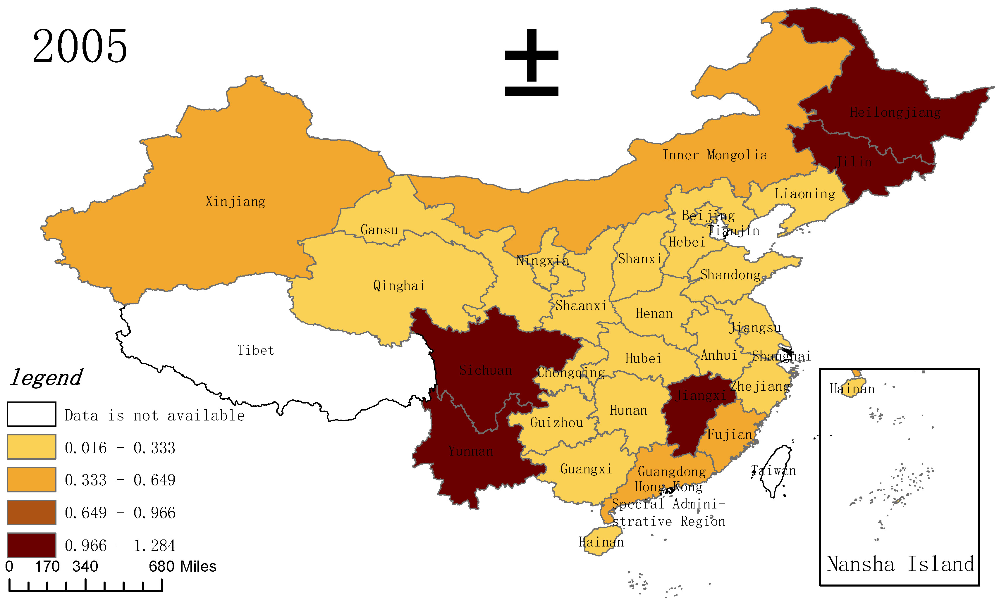
Figure 2.
Spatial distribution of FESE in 2010. Note: “-” is the dash.
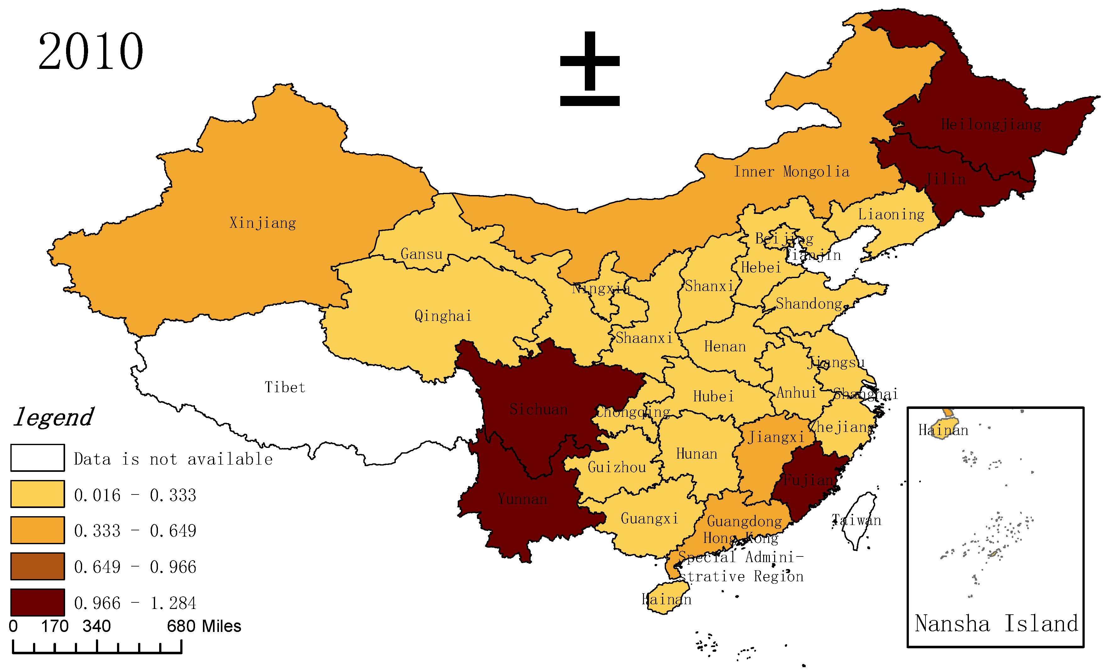
Figure 3.
Spatial distribution of FESE in 2015. Note: “-” is the dash.
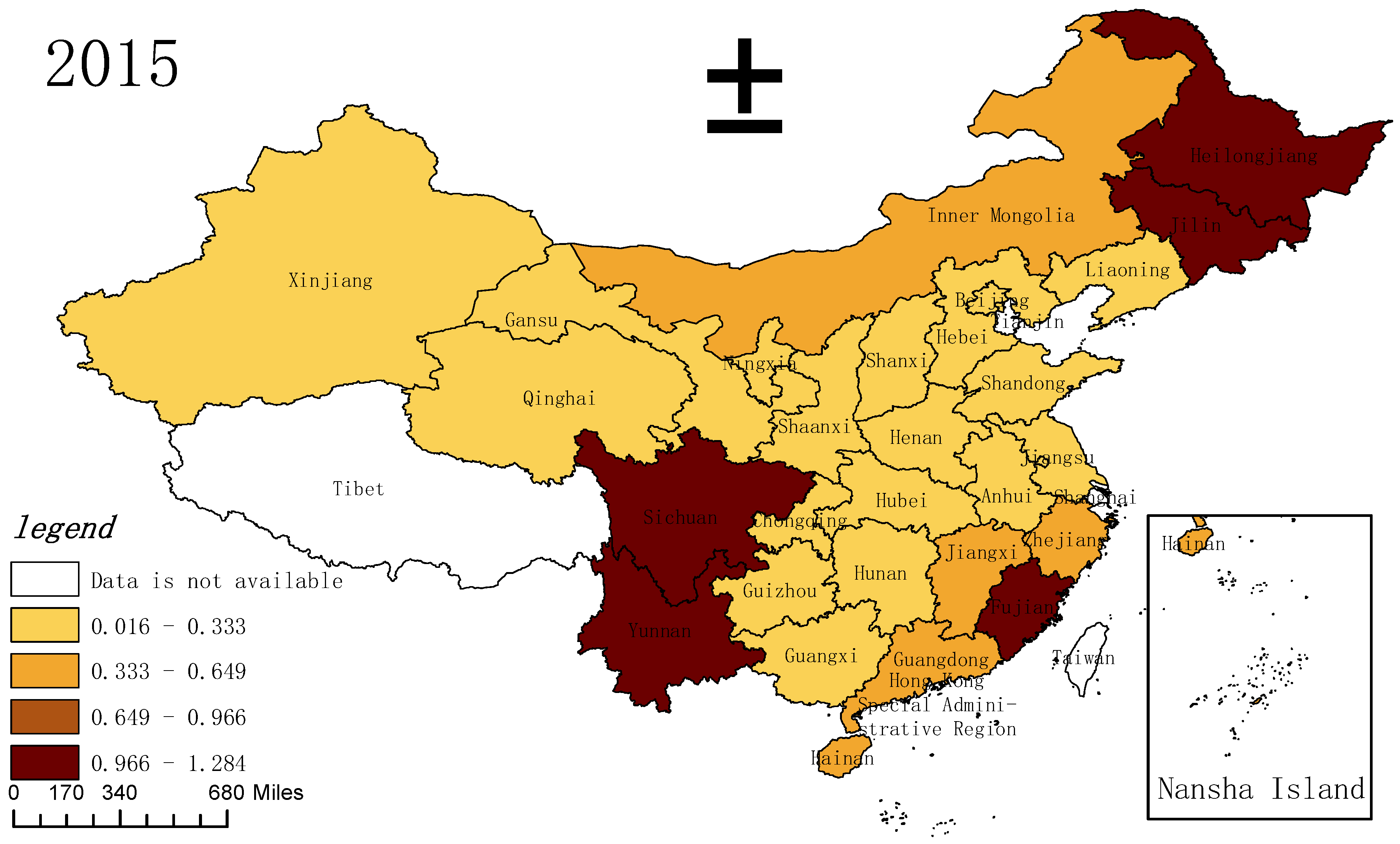
Figure 4.
Spatial distribution of FESE in 2019. Note: “-” is the dash.
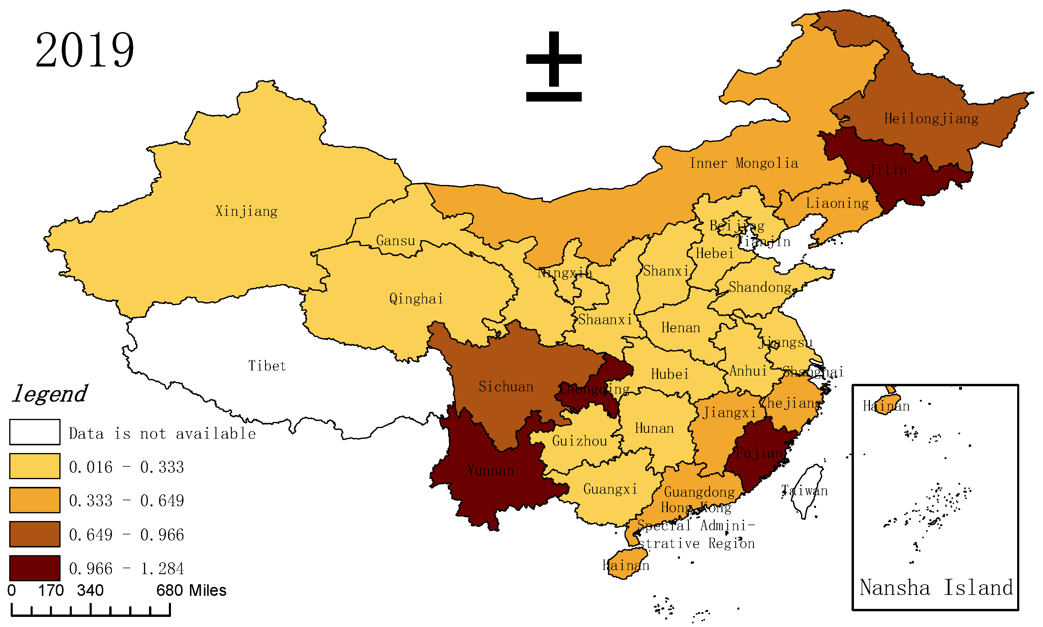
Figure 5.
Spatial distribution of ER in 2005. Note: If there are two “-” between two values, the first “-” is a dash and the rest are minus signs.
Figure 5.
Spatial distribution of ER in 2005. Note: If there are two “-” between two values, the first “-” is a dash and the rest are minus signs.
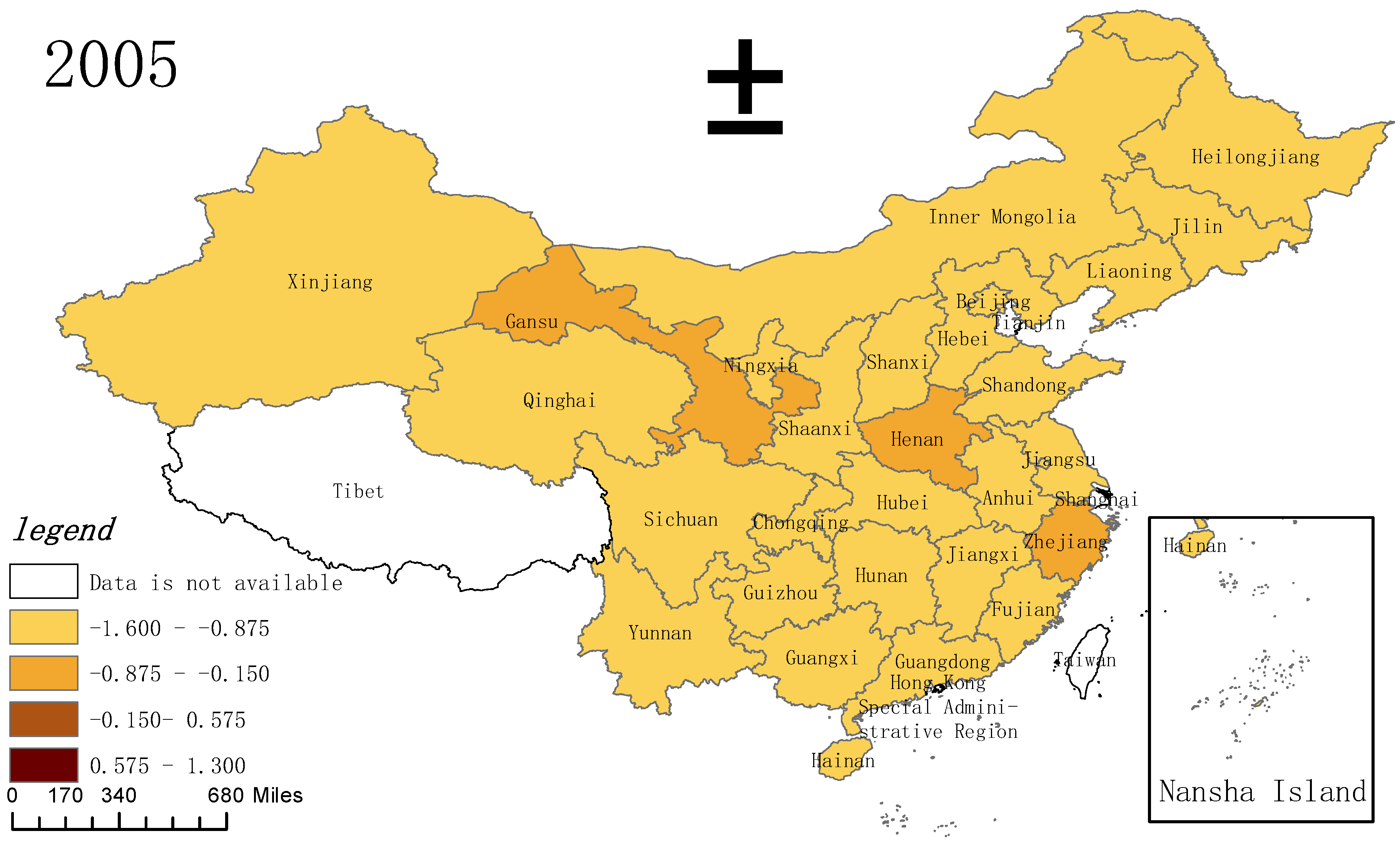
Figure 6.
Spatial distribution of ER in 2010. Note: If there are two “-” between two values, the first “-” is a dash and the rest are minus signs.
Figure 6.
Spatial distribution of ER in 2010. Note: If there are two “-” between two values, the first “-” is a dash and the rest are minus signs.
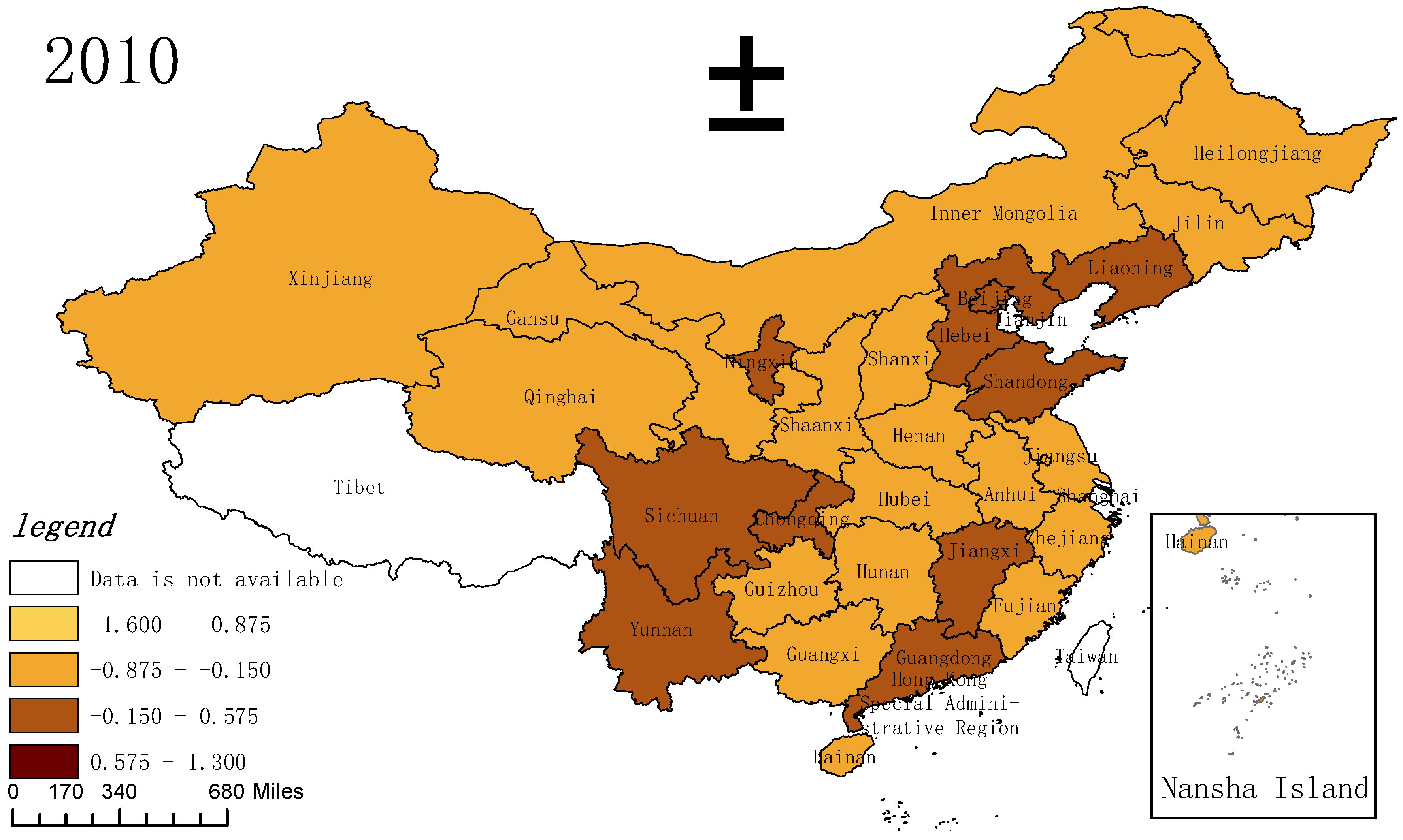
Figure 7.
Spatial distribution of ER in 2015. Note: If there are two “-” between two values, the first “-” is a dash and the rest are minus signs.
Figure 7.
Spatial distribution of ER in 2015. Note: If there are two “-” between two values, the first “-” is a dash and the rest are minus signs.

Figure 8.
Spatial distribution of ER in 2019. Note: If there are two “-” between two values, the first “-” is a dash and the rest are minus signs.
Figure 8.
Spatial distribution of ER in 2019. Note: If there are two “-” between two values, the first “-” is a dash and the rest are minus signs.
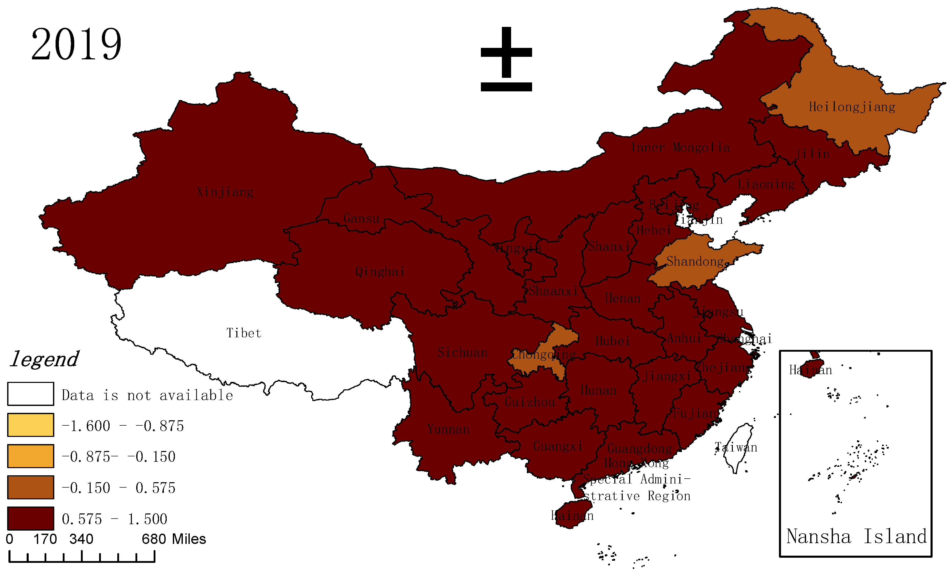
Figure 9.
Local autocorrelation in FESE space in 2005. Note: “-” is the dash.
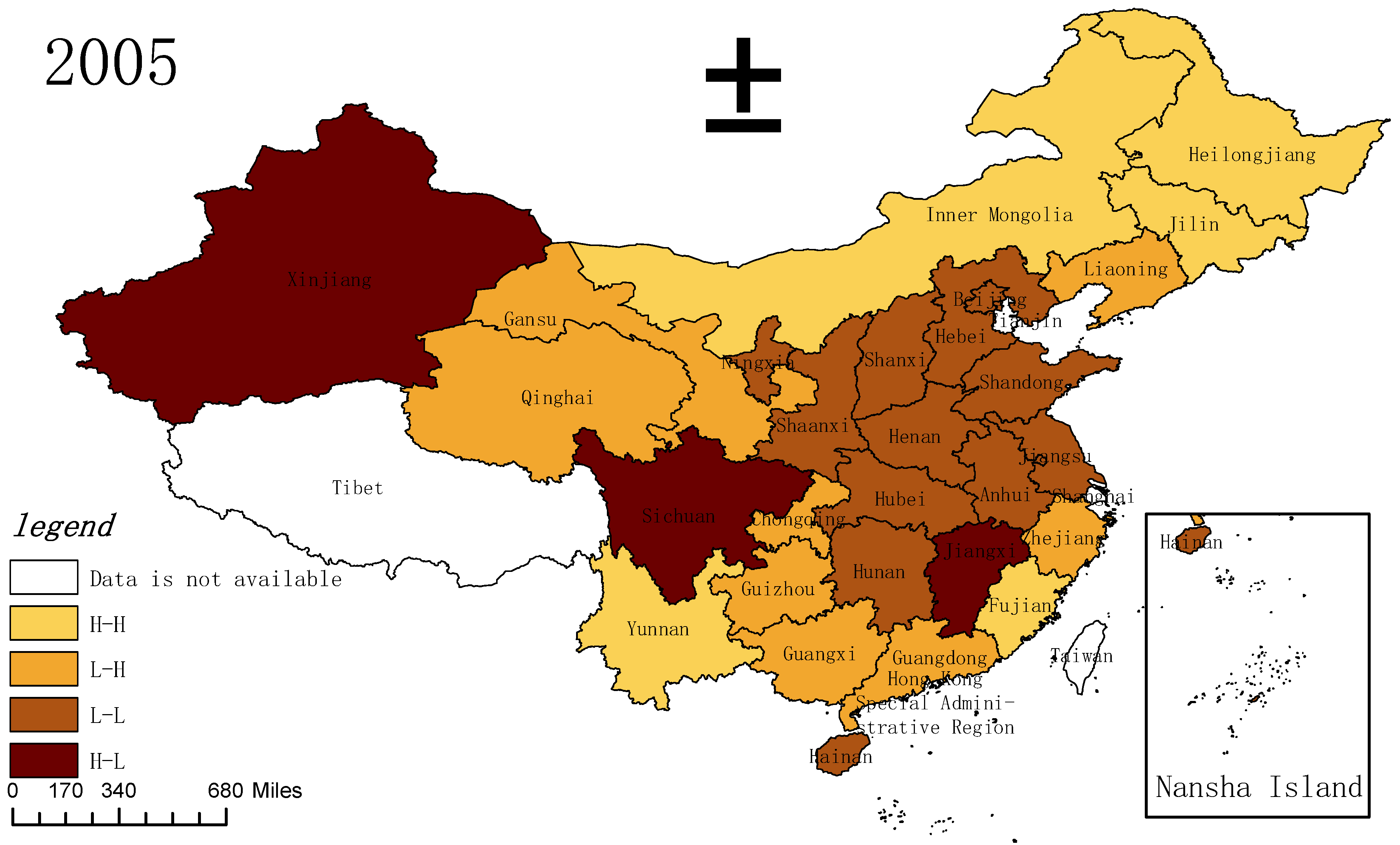
Figure 10.
Local autocorrelation in FESE space in 2010. Note: “-” is the dash.
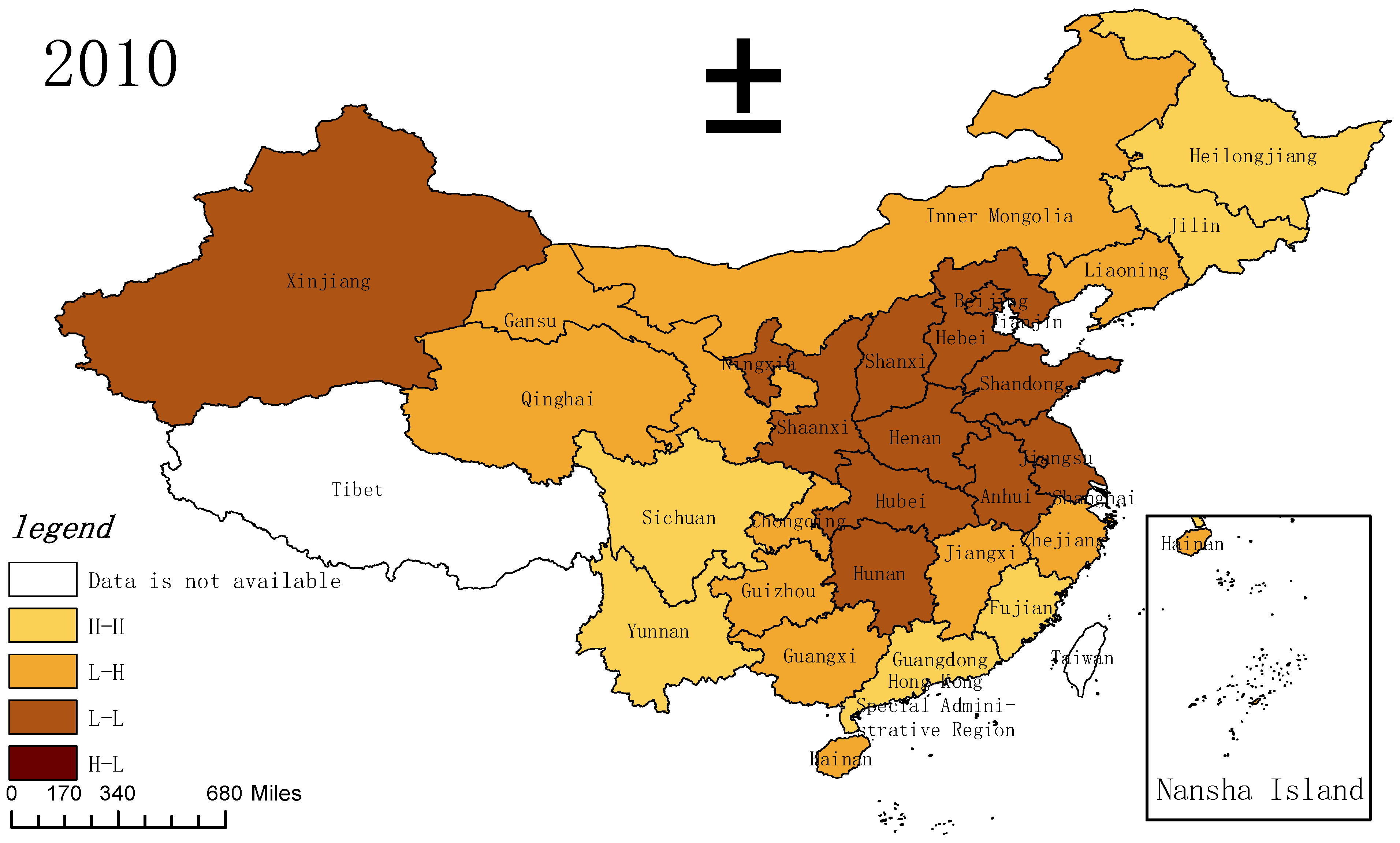
Figure 11.
Local autocorrelation in FESE space in 2015. Note: “-” is the dash.
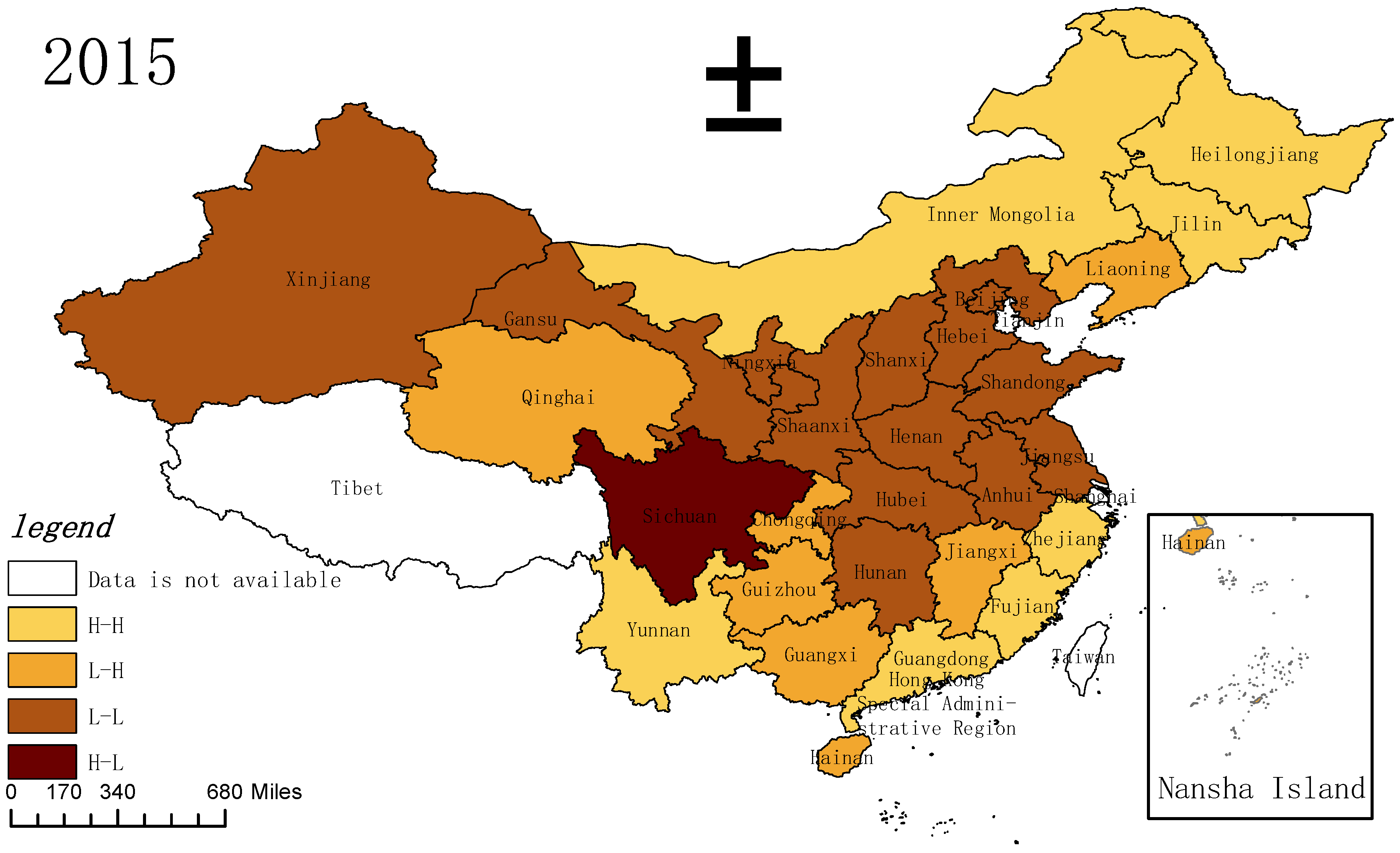
Figure 12.
Local autocorrelation in FESE space in 2019. Note: “-” is the dash.

Table 1.
ER measurement indicators.
| ER | Environmental capacity indicators | Forest cover (%) |
| Afforestation area share (%) | ||
| Environmental governance indicators | The proportion of GDP invested in industrial pollution control (%) | |
| The proportion of GDP invested in environmental infrastructure (%) | ||
| The rate of harmless treatment of domestic waste (%) | ||
| The utilization rate of industrial solid waste (%) | ||
| Environmental pollutant emissions indicators | Carbon dioxide emissions per unit of output value (t/ten thousand yuan) | |
| Sewage emissions per unit of output value (t/ten thousand yuan) |
Table 2.
Input–output indicators for FESE.
| FESE | Input | Capital stock (ten thousand yuan) |
| Land area (ten thousand ha) | ||
| Labor (ten thousand people) | ||
| Expected output | Forest volume (ten thousand m3) | |
| Non-expected outputs | Carbon dioxide emissions (ten thousand tons) |
Table 3.
Descriptive analysis of variables.
| Name | Variables | Sample | Mean | Variance | Minimum | Maximum | VIF |
|---|---|---|---|---|---|---|---|
| Dependent variable | FESE | 420 | 0.395 | 0.376 | 0.016 | 1.289 | |
| Explanatory variables | ER | 420 | 0.000 | 0.689 | −1.550 | 1.500 | 1.68 |
| ER2 | 420 | 0.474 | 0.493 | 0.000 | 2.403 | 1.29 | |
| Other Explanatory Variables | TFESE | 420 | 0.791 | 0.804 | 0.166 | 12.061 | 1.14 |
| SFESE | 420 | 0.573 | 0.304 | 0.007 | 1.000 | 1.61 | |
| TD | 420 | 0.254 | 0.310 | 0.013 | 1.771 | 2.59 | |
| SI | 420 | 0.556 | 0.308 | 0.004 | 1.000 | 1.45 | |
| ST | 420 | 5067 | 9215 | 23 | 59,742 | 2.20 | |
| PS | 420 | 44.406 | 80.536 | 0.298 | 497.647 | 3.37 | |
| LF | 420 | 9.386 | 1.183 | 6.569 | 13.828 | 2.21 | |
| FL | 420 | 5.587 | 4.930 | 0.344 | 35.833 | 1.27 |
Table 4.
Moran’s I efficiency of forestry ecological security from 2005 to 2019.
| Year | Adjacency Matrix | Geographical Distance Matrix | ||
|---|---|---|---|---|
| Moran’s I | p Value | Moran’s I | p Value | |
| 2005 | 0.198 | 0.030 | 0.049 | 0.012 |
| 2006 | 0.250 | 0.010 | 0.067 | 0.003 |
| 2007 | 0.215 | 0.022 | 0.056 | 0.007 |
| 2008 | 0.211 | 0.023 | 0.052 | 0.009 |
| 2009 | 0.224 | 0.018 | 0.054 | 0.008 |
| 2010 | 0.215 | 0.021 | 0.05 | 0.010 |
| 2011 | 0.225 | 0.018 | 0.053 | 0.009 |
| 2012 | 0.239 | 0.014 | 0.058 | 0.006 |
| 2013 | 0.239 | 0.014 | 0.053 | 0.009 |
| 2014 | 0.239 | 0.014 | 0.052 | 0.009 |
| 2015 | 0.234 | 0.015 | 0.052 | 0.009 |
| 2016 | 0.227 | 0.017 | 0.049 | 0.012 |
| 2017 | 0.251 | 0.011 | 0.055 | 0.008 |
| 2018 | 0.318 | 0.002 | 0.074 | 0.002 |
| 2019 | 0.189 | 0.036 | 0.049 | 0.012 |
Table 5.
LM Test.
| Test | LM Value | p Value |
|---|---|---|
| LM_test_lag | 39.991 | 0.000 |
| Robust LM_test_lag | 65.105 | 0.000 |
| LM_test_sem | 0.665 | 0.415 |
| Robust LM_test_sem | 25.779 | 0.000 |
Table 6.
Regression results of spatial econometric model.
| Variables | SAR | SEM | SDM |
|---|---|---|---|
| ER | 0.035 | 0.052 | 0.043 |
| (−0.047) | (−0.048) | (−0.044) | |
| ER2 | −0.075 ** | −0.088 ** | −0.092 *** |
| (−0.037) | (−0.038) | (−0.035) | |
| TFESE | 0.172 *** | 0.184 *** | 0.142 *** |
| (−0.014) | (−0.013) | (−0.013) | |
| SFESE | 1.066 *** | 1.099 *** | 1.037 *** |
| (−0.041) | (−0.040) | (−0.041) | |
| TD | 0.279 *** | 0.340 *** | 0.296 *** |
| (−0.052) | (−0.051) | (−0.050) | |
| SI | 0.035 | 0.108 *** | 0.031 |
| (−0.039) | (−0.041) | (−0.041) | |
| ST | 0.000 | 0.000 * | 0.000 *** |
| (0.000) | (0.000) | (0.000) | |
| PS | 0.000 | 0.000 | 0.001 *** |
| (0.000) | (0.000) | (0.000) | |
| LF | −0.058 *** | −0.061 *** | −0.126 *** |
| (−0.017) | (−0.016) | (−0.019) | |
| FL | 0.002 | −0.001 | 0.003 |
| (−0.002) | (−0.002) | (−0.002) | |
| W × ER | 0.212 ** | ||
| (−0.107) | |||
| W × ER2 | −0.158 * | ||
| (−0.088) | |||
| W × TFESE | 0.046 * | ||
| (−0.027) | |||
| W × SFESE | 0.342 *** | ||
| (−0.115) | |||
| W × TD | 0.378 *** | ||
| (−0.078) | |||
| W × SI | 0.508 *** | ||
| (−0.080) | |||
| W × ST | 0.000 *** | ||
| (0.000) | |||
| W × PS | −0.002 ** | ||
| (−0.001) | |||
| W × LF | 0.054 | ||
| (−0.038) | |||
| W × FL | −0.020 *** | ||
| (−0.006) | |||
| Rho | 0.153 ** () | −0.162 * | |
| (0.061) | (0.084) | ||
| Lambda | −0.277 *** | ||
| (0.082) | |||
| R−squared | 0.686 | 0.683 | 0.617 |
| σ−squared | 0.039 *** | 0.038 *** | 0.031 *** |
| Log−L | 83.620 | 86.001 | 132.271 |
Note: *, ** and *** indicate significant level at 1%, 5%, and 10%, respectively. () is a Std. err.
Table 7.
Spatial effect decomposition.
| Variables | Direct Effects | Indirect Effects | Total Effect |
|---|---|---|---|
| ER | 0.037 | 0.181 * | 0.218 * |
| (−0.044) | (−0.094) | (−0.111) | |
| ER2 | −0.089 *** | −0.124 | −0.213 ** |
| (−0.034) | (−0.084) | (−0.095) | |
| TFESE | 0.143 *** | 0.019 | 0.162 *** |
| (−0.012) | (0.024) | (−0.023) | |
| SFESE | 1.032 *** | 0.158 * | 1.189 *** |
| (−0.041) | (−0.087) | (−0.089) | |
| TD | 0.284 *** | 0.293 *** | 0.578 *** |
| (−0.048) | (0.070) | (−0.081) | |
| SI | 0.015 | 0.451 *** | 0.466 *** |
| (−0.040) | (−0.074) | (−0.084) | |
| ST | 0.000 *** | 0.000 *** | 0.000 *** |
| (0.000) | (0.000) | (0.000) | |
| PS | 0.001 *** | −0.002 ** | −0.001 |
| (0.000) | (−0.001) | (−0.001) | |
| LF | −0.127 *** | 0.065 * | −0.063 ** |
| (−0.020) | (−0.036) | (−0.029) | |
| FL | 0.003 | −0.018 *** | −0.015 ** |
| (−0.002) | (0.006) | (−0.006) |
Note: *, ** and *** indicate significant level at 1%, 5%, and 10%, respectively. () is a Std. err.
Table 8.
Robustness tests for the replacement space matrix.
| Variables | Coef. | Space Coef. | Direct Effects | Indirect Effects | Total Effect |
|---|---|---|---|---|---|
| ER | 0.045 (0.049) | 0.398 (0.358) | 0.038 (0.047) | 0.257 (0.249) | 0.295 (0.270) |
| ER2 | −0.113 *** (0.040) | −0.497 * (0.290) | −0.106 *** (0.037) | −0.303 (0.213) | −0.409 * (0.227) |
| TFESE | 0.137 *** (0.014) | 0.007 (0.072) | 0.140 *** (0.013) | −0.045 (0.043) | 0.095 ** (0.046) |
| SFESE | 1.039 *** (0.040) | 2.095 *** (0.366) | 1.005 *** (0.042) | 1.081 *** (0.243) | 2.086 *** (0.241) |
| TD | 0.338 *** (0.052) | 0.537 (0.483) | 0.329 *** (0.049) | 0.258 (0.322) | 0.587 * (0.330) |
| SI | 0.047 (0.040) | 1.055 *** (0.311) | 0.025 (0.037) | 0.716 *** (0.218) | 0.741 *** (0.228) |
| ST | 0.000 * (0.000) | −0.001 (0.000) | 0.000 * (0.000) | 0.000 (0.000) | 0.000 (0.000) |
| PS | −0.000 (0.000) | −0.005 ** (0.002) | −0.000 (0.000) | −0.003 ** (0.002) | −0.003 ** (0.002) |
| LF | −0.110 *** (0.019) | 0.166 (0.136) | −0.113 *** (0.020) | 0.150 (0.097) | 0.037 (0.089) |
| FL | −0.001 (0.002) | 0.036 (0.024) | −0.001 (0.002) | 0.025 (0.018) | 0.024 (0.018) |
| Rho | −0.510 ** (0.213) | ||||
| σ−squared | 0.031 *** (0.002) | ||||
| R−squared | 0.573 | ||||
Note: *, ** and *** indicate significant level at 1%, 5%, and 10%, respectively. () is a Std. err.
Table 9.
Robustness tests for excluding samples from municipalities.
| Variables | Coef. | Space Coef. | Direct Effects | Indirect Effects | Total Effect |
|---|---|---|---|---|---|
| ER | 0.094 * (0.048) | 0.270 ** (0.113) | 0.088 * (0.049) | 0.236 ** (0.102) | 0.324 *** (0.122) |
| ER2 | −0.095 ** (0.038) | −0.226 ** (0.089) | −0.091 ** (0.037) | −0.194 ** (0.089) | −0.285 *** (0.102) |
| TFESE | 0.145 *** (0.013) | 0.050 * (0.027) | 0.146 *** (0.013) | 0.028 (0.025) | 0.174 *** (0.025) |
| SFESE | 1.048 *** (0.045) | 0.203 * (0.119) | 1.047 *** (0.045) | 0.077 (0.093) | 1.124 *** (0.098) |
| TD | 0.304 *** (0.066) | 0.430 *** (0.090) | 0.293 *** (0.064) | 0.361 *** (0.083) | 0.655 *** (0.099) |
| SI | 0.050 (0.044) | 0.722 *** (0.093) | 0.032 (0.043) | 0.661 *** (0.094) | 0.694 *** (0.112) |
| ST | −0.000 (0.000) | 0.000 *** (0.000) | -0.000 (0.000) | 0.000 *** (0.000) | 0.000 ** (0.000) |
| PS | 0.004 *** (0.001) | −0.003 * (0.002) | 0.004 *** (0.001) | −0.003 * (0.002) | 0.001 (0.001) |
| LF | −0.148 *** (0.021) | 0.062 (0.040) | −0.149 *** (0.021) | 0.071 * (0.039) | −0.077 ** (0.033) |
| FL | 0.000 (0.003) | −0.022 *** (0.007) | 0.001 (0.002) | −0.020 *** (0.007) | −0.019 ** (0.008) |
| Rho | −0.116 (0.084) | ||||
| σ−squared | 0.031*** (0.002) | ||||
| R−squared | 0.535 | ||||
Note: *, ** and *** indicate significant level at 1%, 5%, and 10%, respectively. () is a Std. err.
Disclaimer/Publisher’s Note: The statements, opinions and data contained in all publications are solely those of the individual author(s) and contributor(s) and not of MDPI and/or the editor(s). MDPI and/or the editor(s) disclaim responsibility for any injury to people or property resulting from any ideas, methods, instructions or products referred to in the content. |
© 2023 by the authors. Licensee MDPI, Basel, Switzerland. This article is an open access article distributed under the terms and conditions of the Creative Commons Attribution (CC BY) license (https://creativecommons.org/licenses/by/4.0/).
Share and Cite
MDPI and ACS Style
Lu, H.; Zhang, M.; Nian, W. The Spatial Spillover Effects of Environmental Regulations on Forestry Ecological Security Efficiency in China. Sustainability 2023, 15, 1875. https://doi.org/10.3390/su15031875
AMA Style
Lu H, Zhang M, Nian W. The Spatial Spillover Effects of Environmental Regulations on Forestry Ecological Security Efficiency in China. Sustainability. 2023; 15(3):1875. https://doi.org/10.3390/su15031875
Chicago/Turabian StyleLu, Hongliang, Min Zhang, and Wei Nian. 2023. "The Spatial Spillover Effects of Environmental Regulations on Forestry Ecological Security Efficiency in China" Sustainability 15, no. 3: 1875. https://doi.org/10.3390/su15031875
Note that from the first issue of 2016, this journal uses article numbers instead of page numbers. See further details here.