Toward 30 m Fine-Resolution Land Surface Phenology Mapping at a Large Scale Using Spatiotemporal Fusion of MODIS and Landsat Data

Abstract

Satellite-retrieved land surface phenology (LSP) is a first-order control on terrestrial ecosystem productivity, which is critical for monitoring the ecological environment and human and social sustainable development. However, mapping large-scale LSP at a 30 m resolution remains challenging due to the lack of dense time series images with a fine resolution and the difficulty in processing large volumes of data. In this paper, we proposed a framework to extract fine-resolution LSP across the conterminous United States using the supercomputer Tianhe-2. The proposed framework comprised two steps: (1) generation of the dense two-band enhanced vegetation index (EVI2) time series with a fine resolution via the spatiotemporal fusion of MODIS and Landsat images using ESTARFM, and (2) extraction of the long-term and fine-resolution LSP using the fused EVI2 dataset. We obtained six methods (i.e., AT, FOD, SOD, RCR, TOD and CCR) of fine-resolution LSP with the proposed framework, and evaluated its performance at both the site and regional scales. Comparing with PhenoCam-observed phenology, the start of season (SOS) derived from the fusion data using six methods of AT, FOD, SOD, RCR, TOD and CCR obtained r values of 0.43, 0.44, 0.41, 0.29, 0.46 and 0.52, respectively, and RMSE values of 30.9, 28.9, 32.2, 37.9, 37.8 and 33.2, respectively. The satellite-retrieved end of season (EOS) using six methods of AT, FOD, SOD, RCR, TOD and CCR obtained r values of 0.68, 0.58, 0.68, 0.73, 0.65 and 0.56, respectively, and RMSE values of 51.1, 53.6, 50.5, 44.9, 51.8 and 54.6, respectively. Comparing with the MCD12Q2 phenology, the satellite-retrieved 30 m fine-resolution LSP of the proposed framework can obtain more information on the land surface, such as rivers, ridges and valleys, which is valuable for phenology-related studies. The proposed framework can yield robust fine-resolution LSP at a large-scale, and the results have great potential for application into studies addressing problems in the ecological environmental at a large scale.

1. Introduction

Land surface phenology (LSP) is a first-order control on terrestrial ecosystem productivity through altering albedo, surface roughness length and evapotranspiration [1], which plays a key role in energy exchange, water cycle of the earth’s system and carbon balance [2,3,4,5,6,7,8]. In the context of global warming, effective and reasonable control of carbon has become one of the core issues of ecological environmental sustainable development [9]. Therefore, characterizing seasonal and annual land surface dynamics is critical for monitoring ecological environment and human and social sustainable development [10,11,12].

The satellite remote sensing data with rich historical records and suitable spatial-temporal resolutions are frequently employed to monitor the variation of LSP [4,11,13,14]. The satellite-retrieved vegetation phenology termed LSP [10,15,16] has great application potential for characterizing the seasonal and annual land surface dynamics, such as monitoring the climate-vegetation interaction, modeling the carbon cycles, crop-type discrimination, crop yield estimation and land cover mapping [13,17,18,19,20,21,22]. Based on satellite remote sensing data, many methods for retrieving LSP have been developed, such as the amplitude threshold (AT) [23,24], first-order derivative (FOD) [25], second-order derivative (SOD) [26], relative change rate (RCR) [27], third-order derivative (TOD) [28] and curvature change rate (CCR) [29]. These methods provide basic algorithms for satellite remote sensing vegetation phenology research. Most previous studies used these methods to obtain the coarse-resolution LSP (250 m to 8000 m) from coarse-resolution satellite data (such as AVHRR, MODIS, SPOT VGT) [3,4,30,31]. In the coarse-resolution images, each pixel reflects the average phenophase for various types of vegetation within a large coverage. The mixed pixel and scale effect lead to noticeable uncertainties in the satellite-retrieved phenology [32]. Fine-resolution phenology can be helpful for reducing the uncertainties caused by the mixed pixel and scale effect, and provide more spatially detailed information of the land surface.

However, mapping large-scale LSP at a fine-resolution faces at least the following two challenges [20,33]. Firstly, LSP extraction requires remote sensing images with both high temporal and spatial resolution, but this need cannot be satisfied by a single satellite sensor due to the tradeoffs between the temporal and spatial resolution. For example, the most commonly used Landsat has a fine spatial resolution (30 m), while its revisiting cycle is up to 16 days. In practice, the cloudy weather conditions would further reduce the temporal resolution of the Landsat time series data. Recently, some research employed the harmonized Landsat Sentinel-2 (HLS) product to retrieve fine-spatial resolution phenology [3,20]. However, the HLS product can only be used to retrieve the phenology from 2015 to the present due to the lack of historical records. Secondly, the high temporal-spatial resolution images at large scales are regarded as Big Data, the difficulties in data processing and the limitation of computing resources greatly limit the application scenarios. As a result, existing research has mainly focused on extracting fine-resolution LSP at a small scale. For example, Melaas, et al. [34,35] used Landsat TM/ETM+ data to retrieve phenology from some deciduous broadleaf in Canada and the Eastern United States. Li, et al. [36] applied the double logistic model to fit the two-band enhanced vegetation index (EVI2) time series from Landsat images, and then used it to retrieve the LSP for some urban areas in the conterminous United States from 1985 to 2015.

Obtaining high temporal and spatial resolution data for retrieving LSP, the solutions may include: (1) generating a harmonized dataset via the combination of multiple high-resolution sensors, e.g., the HLS product [3,20]; (2) blending high temporal resolution but low spatial resolution data (such as MODIS) and high spatial resolution but low temporal resolution data (such as Landsat, Sentienl-2) to obtain high spatial resolution and dense time-series data [37,38]. Among them, the enhanced spatial and temporal adaptive reflectance fusion model (ESTARFM) [38] is widely used in the spatiotemporal fusion of multisource images. ESTARFM has proved to be effective in blending MODIS and Landsat images, especially in heterogeneous landscapes. However, the application of ESTARFM at a large scale remains challenging, due to the requirement of a huge amount computing resources.

The goal of this study is to achieve 30 m fine-resolution LSP mapping at a large scale using spatiotemporal fusion of MODIS and Landsat data. To achieve this goal, we developed a framework, which integrates six LSP extraction methods of amplitude threshold (AT), first-order derivative (FOD), second-order derivative (SOD), relative change rate (RCR), third-order derivative (TOD) and curvature change rate (CCR). The proposed framework can yield robust fine-resolution LSP at a large-scale via the spatiotemporal fusion of MODIS and Landsat images using supercomputer Tianhe 2, and it provides a strategy for selecting the input images to reduce impact from clouds.

2. Materials and Methodology

2.1. Landsat Data

We selected the red band and near-infrared (NIR) band of Landsat 8 data from 2013 to 2018 as fine-resolution data for spatiotemporal fusion. We only used the Landsat 8 images and the corresponding MODIS images both with a cloud cover of less than 10% and it was necessary that the selected image included at least one PhenoCam site for validation. The operational land imager (OLI) sensor of Landsat 8 has 9 spectral bands, and the scene size of Landsat 8 is 185 km × 180 km. The orbit gives a repeat cycle of 16 days and the altitude of the satellite is 705 km. As shown in Figure 1, it takes about 470 tiles of Landsat images to fully cover the conterminous United States. In this study, we acquired the USGS Landsat 8 Surface Reflectance Tier 1 from the Google Earth Engine (GEE, https://earthengine.google.com/) platform. With the GEE platform, we performed the pre-processing of the images before downloading.

2.2. MODIS Data

We employed MODIS/Terra Surface Reflectance 8-day 250 m product (MOD09Q1, Version 6) as the coarse-resolution images for spatiotemporal fusion [39]. MOD09Q1 includes two surface reflectance bands (red band, 620–670 nm; near-infrared band, 841–876 nm) with 8-day temporal resolution and about 250 m spatial resolution. The MODIS/Terra and Aqua Land Cover Dynamics Yearly L3 Global 500 m SIN Grid (MCD12Q2, Version 6), which provides vegetation phenology over global land surfaces [40], was used as reference data for evaluating the performance of 30 m fine-resolution phenology. Both MOD09Q1 and MCD12Q2 are available from https://search.earthdata.nasa.gov/. In this research, we only retrieved two commonly used phenology metrics (i.e., SOS and EOS). So, in MCD12Q2 data, we used the greenup layer (i.e., SOS) and the dormancy layer (i.e., EOS) for analysis. In the MCD12Q2 product, the SOS and the EOS are acquired when EVI2 first crosses the 15% amplitude of the corresponding segment EVI2 time series.

2.3. PhenoCam Data

We used the PhenoCam Dataset v2.0 [41] as validation data for evaluating the performance of the land surface phenophases extracted from the fused EVI2 time series. The PhenoCam sites were established in 2008, which used the networked digital camera to track vegetation phenology, and it has about 500 sites mainly located in North America. The PhenoCam Dataset v2.0 [41] can be obtained from https://phenocam.sr.unh.edu/webcam/, and it provides the time series of vegetation phenological observations for diverse ecosystems, such as agriculture, deciduous broadleaf forests, deciduous needleleaf forests, evergreen broadleaf forests, grasslands, mixed vegetation, shrubs, tundra vegetation and wetland vegetation. Considering the unstable phenological changes of some ecosystems (such as agriculture and evergreen broadleaf forests) and the cloud cover situation of satellite observations, we only selected the PhenoCam sites that were located in the Landsat 8 images with a cloud cover of less than 10 percent. So, we employed the phenology records of the deciduous broadleaf forest (DBF) sites, shrubland (SHR) sites and grassland (GRA) sites from 2013 to 2018 for the satellite-retrieved phenology validation, as shown in Figure 2. Three threshold values (i.e., 10%, 25% and 50%) of the green chromatic coordinate index mean (G_cc-mean) were employed to retrieve the vegetation phenophases from the PhenoCam Dataset. The threshold value of 50% for the vegetation index time series is rarely used to retrieve vegetation phenophases from remote sensing data, and the SOS and EOS retrieved with threshold values of 10% and 25% of the vegetation index time series are similar [42]. Thus, the SOS and EOS of the PhenoCam Dataset v2.0 with threshold values of 25% of the G_cc-mean amplitude were selected for validation.

2.4. Supercomputer-Tianhe-2

Mapping large-scale LSP with 30 m spatial resolution requires massive computing resources, and the general computers cannot meet the demand. In this study, we used supercomputer Tianhe-2 for blending Landsat 8 and MOD09Q1 data for extracting the LSP. Tianhe-2 is a supercomputer developed by China, and it is located in the “National Supercomputing Guangzhou Center” at Sun Yat-sen University, Guangzhou. Tianhe-2 contains approximately 17, 920 computing nodes, which gives a theoretical peak performance of 54.9 quadrillion floating-point operations per second (petaFLOPS) and an actual performance of 33.9 petaFLOPS. In 2013–2015, Tianhe-2 ranked first in the world six consecutive times, and it won four consecutive championships in the high-performance conjugate gradient benchmark. In this study, we employed 5 graphic processing unit (GPU) nodes and 64 central processing unit (CPU) nodes of Tianhe-2. Each GPU node contains 4 Tesla k80 graphics cards, and each CPU node includes an Intel(R) Xeon(R) CPU E5-2660 v3 @ 2.60 GHz with 256 gigabyte of running memory. For each Landsat image, it took about 6 h to generate high spatiotemporal resolution data and extracted the vegetation phenology, and were able to process 20 Landsat images synchronously.

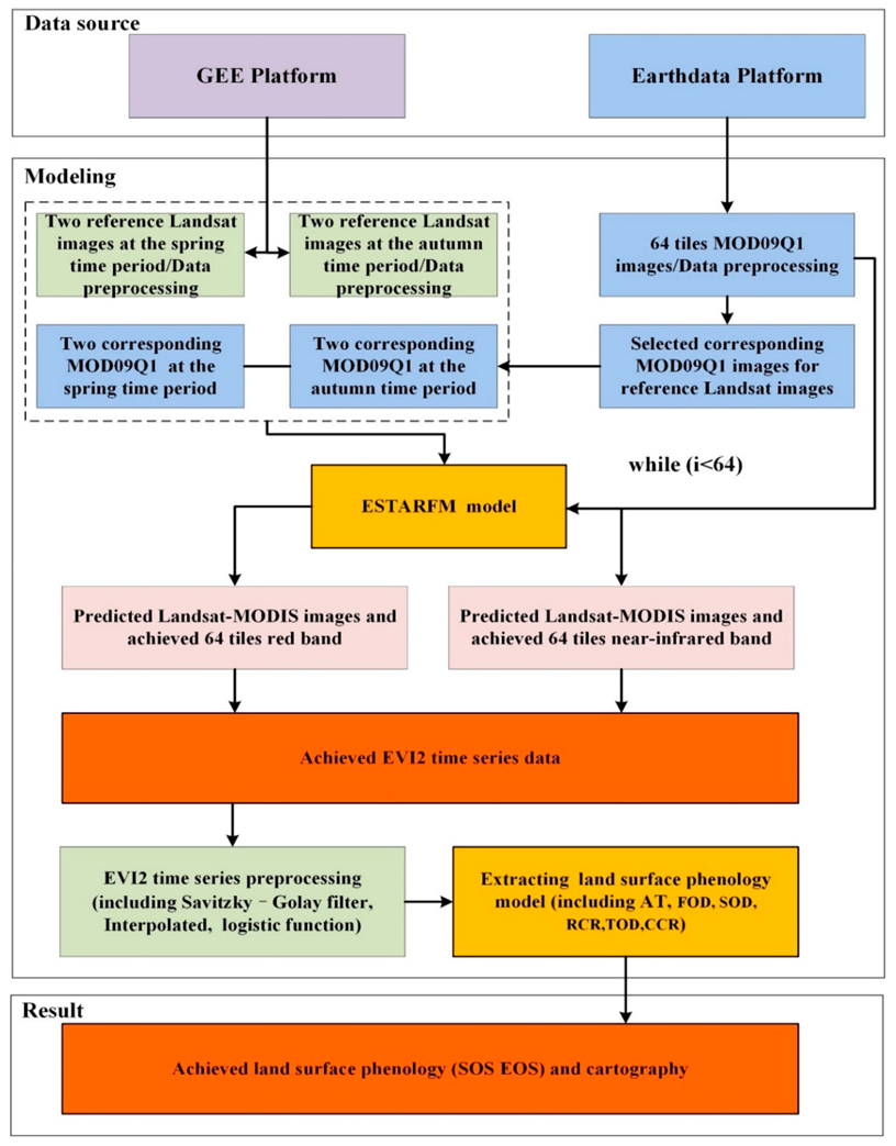
2.5. Generating High Spatiotemporal Resolution Images

We used ESTARFM to blend Landsat and MODIS data and generate dense time-series images with 30 m resolution. ESTARFM requires a coarse-resolution image on the prediction date and two reference coarse-fine resolution image pairs in the neighboring dates to predict the fine-resolution image on the prediction date [38]. The precondition of using ESTARFM for generating spatiotemporal fusion data from multi-source satellite data is that the coarse-resolution sensor has similar spectral bands as the fine-resolution sensor, such as the red band and near-infrared band of Landsat with the red band and near-infrared band of MODIS. ESTARFM then uses the correlation to blend multi-source satellite data (coarse-resolution and fine-resolution) while minimizing the system bias. Moreover, according to the heterogeneity of the land surfaces, the ESTARFM adopts different processing schemes for mixed pixels and pure pixels. ESTARFM assumes that surface reflectance changes linearly, which is inconsistent with the growth pattern of natural vegetation. To reduce the blending errors, we divided the growth cycle into growth period (January 1 to June 30) and dormancy period (July 1 to December 31), and set up a rule to select two appropriate reference Landsat images for each period.

First, we sorted the Landsat images in an ascending order according to the cloud cover (CC). These images were then classified into three categories, i.e., good-quality images (CC < 10%), medium-quality images (10% ≤ CC ≤ 50%) and low-quality images (CC > 50%). The good-quality images were used as reference. If the number of good-quality images was not enough (4 images), then we filled the missing pixels in the medium-quality image with the counterparts of its neighboring two images and used the filled images as reference.

In tropical or subtropical regions, it is often the case that only 1 reference image is available due to the frequent rain weather. In such cases, we simply copied it to fulfill the image quantity requirements of ESTARFM. We filled all of the cloud pixels of the Landsat image with a 0 value. The selection of the reference Landsat images was conducted in the GEE platform. For the 8-day MOD09Q1 data, we chose the image with the date closest to the date of the input Landsat images. If the fine-resolution input image was composed of multiple Landsat images, then the corresponding coarse-resolution input image was also composed of the corresponding multiple MODIS images. Then, we downloaded the reference Landsat/MODIS images and performed spatiotemporal fusion using Tianhe-2.

2.6. The Framework for Extracting LSP from Fused Landsat-MODIS Data

Note that the phenophases of some vegetation in the conterminous United States may appear in the previous year (SOS) or the following year (EOS). For each year, we used 64 fused Landsat-MODIS images for extracting LSP, including 46 images acquired in the current year, 9 images acquired in the previous year (i.e., the 297th, 305th, 313th, 321th, 329th, 337th, 345th, 353th and 361th days of the previous year) and 9 images in the following year (i.e., the 1th, 9th, 17th, 25th, 33th, 41th, 49th, 57th, and 65th days of the following year).

We obtained the EVI2 time series data from the fused Landsat-MODIS images, as the following equation:

$$EVI2=2.5\frac{{\rho }_N-{\rho }_R}{{\rho }_N+2.4{\rho }_R+1}$$

(1)

where EVI2 denotes the two-band enhanced vegetation index, ${\rho }_N$ denotes the near-infrared band reflectance, ${\rho }_R$ denotes the red band reflectance.

We used the Savitzky–Golay (S–G) method [43] to remove the outliers of the EVI2 time series, and interpolated the 8-day EVI2 time series to 1-day intervals. We divided the EVI2 time series of a growing season into growth period and dormancy period, and used Equation (2) to fit them.

$$y\left(t\right)=\frac{c}{1+e^{a+bt}}+d$$

(2)

where t denotes the day of the year, $y\left(t\right)$ denotes the EVI2 value on date t, a, b, c and d are fitting parameters. We resorted the data series data when fitting the EVI2 of vegetation dormancy with Equation (2) (See

Table 1. Description of the six methods for extracting the start of season (SOS) and end of season (EOS) from the EVI2 time series.

Method	Index	SOS	EOS	Reference
Amplitude threshold	AT	$0.2\times \left(\max \left(\mathrm{EVI}{2}_s\right)-\min \left(\mathrm{EVI}{2}_s\right)\right)$	$0.2\times \left(\max \left(\mathrm{EVI}{2}_a\right)-\min \left(\mathrm{EVI}{2}_a\right)\right)$	[24]
First-order derivative	FOD	$\max \left(dt\left(\mathrm{EVI}{2}_s\right)\right)$	$\min \left(dt\left(\mathrm{EVI}{2}_a\right)\right)$	[25]
Second-order derivative	SOD	$\max \left(d{t}^2\left(\mathrm{EVI}{2}_s\right)\right)$	$\max \left(d{t}^2\left(\mathrm{EVI}{2}_a\right)\right)$	[26]
Relative change rate	RCR	$\max \left(\frac{\mathrm{EVI}{2}_s\left(t+1\right)-\mathrm{EVI}{2}_s\left(t\right)}{\mathrm{EVI}{2}_s\left(t\right)}\right)$	$\min \left(\frac{\mathrm{EVI}{2}_a\left(t+1\right)-\mathrm{EVI}{2}_a\left(t\right)}{\mathrm{EVI}{2}_a\left(t\right)}\right)$	[27]
Third-order derivative	TOD	$\max \left(d{t}^3\left(\mathrm{EVI}{2}_s\right)\right)$	$\min \left(d{t}^3\left(\mathrm{EVI}{2}_a\right)\right)$	[28]
Curvature change rate	CCR	$\max \left({K^{\prime }}_s\left(t\right)\right)$	$\max \left({K^{\prime }}_a\left(t\right)\right)$	[29]

Note: where $\mathrm{EVI}{2}_s$ represents EVI2 at the periods of sustained increase for the phenological cycles (i.e., spring); $\mathrm{EVI}{2}_a$ represents EVI2 at the periods of sustained decrease for the phenological cycles (i.e., autumn); t represents the day of the year in the EVI2 time series; ${K^{\prime }}_s$ represents the rate of change of the curvature of the logistic-fitted EVI2 time series during the periods of sustained increase for the phenological cycles (i.e., spring); ${K^{\prime }}_a$ represents the rate of change of curvature of the logistic-fitted EVI2 time series during the periods of sustained decrease for the phenological cycles (i.e., autumn) (for more details, please see [29]); max() and min() denote the maximum and minimum of the time series data, respectively; and $dt()$ and $d{t}^3()$ denote obtaining the first-order, second-order and third-order derivatives of the time series data, respectively.

).

The Figure 3 shows the framework for extracting the fine-resolution LSP. This framework is mainly divided into three parts consisting of data source, modeling and result. Firstly, we downloaded the Landsat images and MOD09Q1 images from the GEE platform and the Earthdata platform, and at the same time, we began data preprocessing. Secondly, we fed the Landsat and MODIS data into the ESTARFM model for obtaining the Landsat-MODIS and the EVI2 time series data. In a phenological period, we repeated step 2 until the ESTARFM model generated 64 tiles of fine-resolution fusion images. Finally, we used the extraction LSP model to obtain the fine-resolution phenology mapping. Note that in this research, land cover/land use data is not used as a basis for the extraction of the phenological characteristics or used to process the LSP mapping.

3. Results

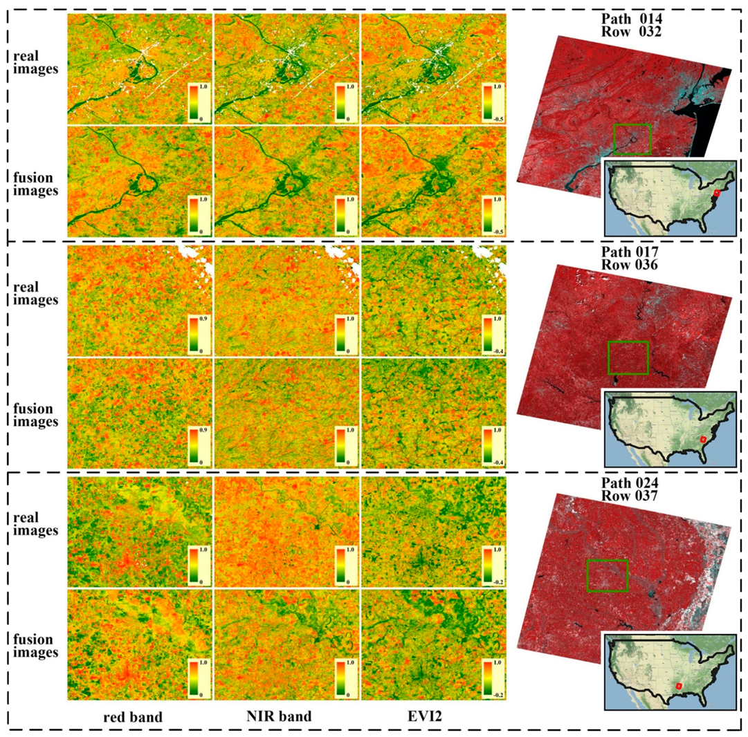
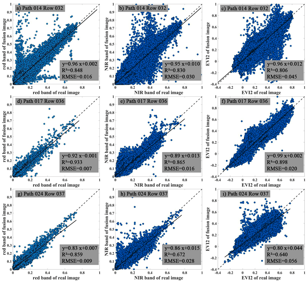
3.1. The Performance of the Data Fusion with ESTARFM

We used ESTARFM for fusing the Landsat and MOD09Q1 images to obtain the fine spatiotemporal resolution dataset. Figure 4 shows the red band, near infrared (NIR) band and extracted EVI2 from the fused dataset in three tiles, i.e., Path 014 Row 032, Path 017 Row 036 and Path 024 Row 037. We selected an area of 50 km × 50 km from the three images for comparison of the difference between the real images and the simulation images. It was found that the fused image of Path 014 Row 032 and Path 017 Row 036 were similar with the real Landsat. As for Path 024 Row 037, the red band of the fused image was overestimated, and the near-infrared band and EVI2 were underestimated, as compared with the real Landsat image. Overall, the images fused using the proposed reference image selection rule have similar spatial distribution characteristics with the real ones.

Figure 5 shows the scatterplots for the regression analysis between the real Landsat images and the fused images in the selected 50 km × 50 km rectangles, as marked in Figure 4 (over 2 million pixels). Among them, Figure 5a,d,g are the regression analysis between the red bands from real Landsat and fused images. The fused red bands achieved the R² value of 0.848, 0.933 and 0.859, and the RMSE value of 0.016, 0.007 and 0.009, respectively, in the three selected areas. Figure 5b,e,h are the regression analysis between the NIR bands from the real Landsat and fused images. The fused NIR band achieved an R² value of 0.830, 0.865 and 0.672, and an RMSE value of 0.030, 0.016 and 0.028, respectively, in the three selected areas. Figure 5c,f,i shows the regression analysis between the EVI2 derived from the real Landsat and fused images. The fused EVI2 achieved an R² value of 0.806, 0.898 and 0.640, and an RMSE value of 0.045, 0.020 and 0.056, respectively. From Figure 5, the RMSE values of both the red bands, the near-infrared band and the EVI2 are all less than 0.06, indicating that the proposed reference image selection rule leads to an accurate fusion result.

In order to understand the performance of the EVI2 time series calculated by the fused dataset, we selected 6 points for investigating, three of them were near the urban area and the others were from the forest area). The coordinates of the 6 points from the Point 1 to the Point 6 in Figure 6 are (Lat 42.978°, Lon −72.720°), (Lat 42.967°, Lon −72.721°), (Lat 42.973°, Lon −72.707°), (Lat 42.910°, Lon −72.275°), (Lat 42.911°, Lon −72.287°) and (Lat 42.905°, Lon −72.293°), respectively. In Figure 6, the gray points are the EVI2 calculated by the fused dataset, the red points are the EVI2 calculated by the real Landsat images. The green and orange curves denote the growth and dormancy periods extracted by the growth logistic function, respectively. In Figure 6, it can be seen that the difference between the real Landsat EVI2 and fused EVI2 is small. Furthermore, the fused EVI2 time series reflects well the tendency of the phenological cycles from growth to dormancy. There results indicate that the proposed reference image selection rule is effective and robust.

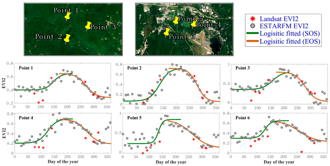
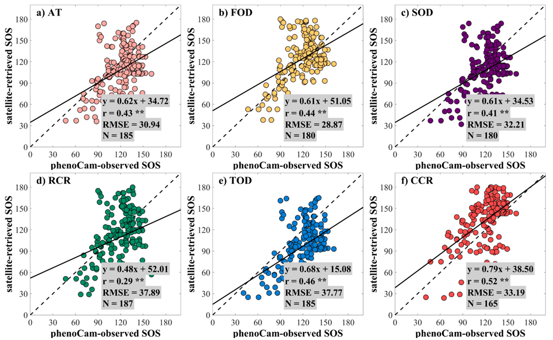
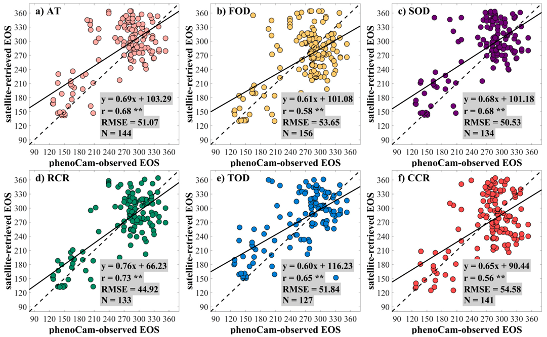
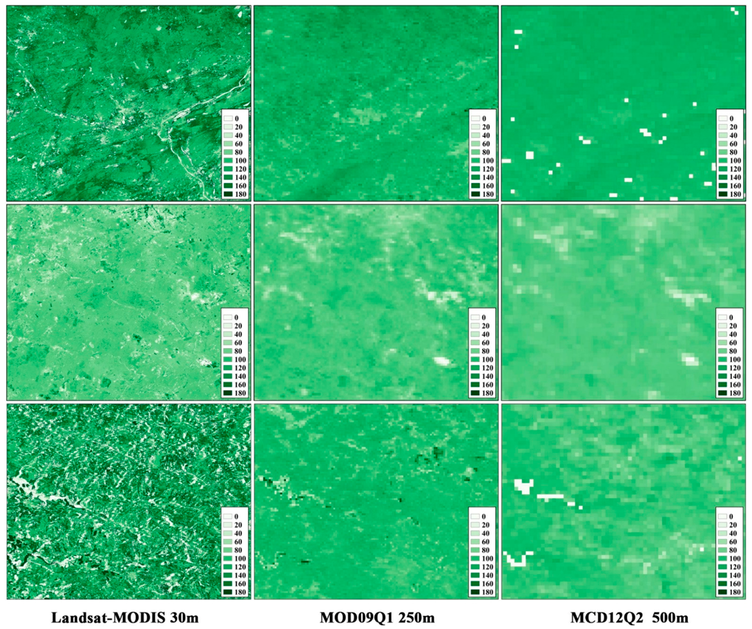
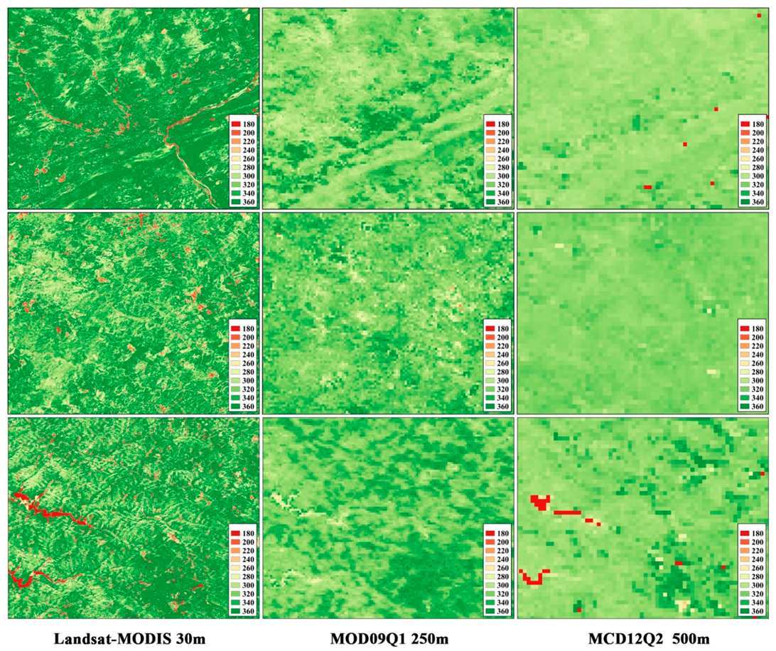
3.2. The Performance of Extracting LSP from the Fused EVI2 Time Series

Once the EVI2 time series from fused dataset was obtained, we used six methods (AT, FOD, SOD, RCR, TOD and CCR) to retrieve the 30 m spatial resolution LSP from 2003 to 2018 (in the year of 2013 to 2016, we only extracted the LSP from the PhenoCam locations), and evaluated the retrieved LSP using PhenoCam-observed phenology. Figure 7 shows the scatterplots for the regression analysis between the PhenoCam-observed SOS and the satellite-retrieved SOS using the methods of AT, FOD, SOD, RCR, TOD and CCR. In Figure 7, most points are around the 1:1 line, demonstrating that SOS derived from two independent datasets are consistent. Compared with PhenoCam-observed SOS, the SOS derived from the fused EVI2 by the six methods of AT, FOD, SOD, RCR, TOD and CCR, obtained r values of 0.43, 0.44, 0.41, 0.29, 0.46 and 0.52, and RMSE values of 30.94, 28.87, 32.21, 37.89, 37.77 and 33.19, respectively. Overall, the CCR method obtained the worst SOS and the other methods had a similar performance.

Figure 8 shows the scatterplots for the regression analysis between the PhenoCam-observed EOS and the satellite-retrieved EOS using the methods of AT, FOD, SOD, RCR, TOD and CCR. Most points in Figure 8 are around the 1:1 line, but they are more discrete than the SOS scatter points, as shown in Figure 7. Compared with the PhenoCam-observed EOS, the EOS derived from the fused EVI2 by the six methods of AT, FOD, SOD, RCR, TOD and CCR obtained r values of 0.68, 0.58, 0.68, 0.73, 0.65 and 0.56, and RMSE values of 51.07, 53.65, 50.53, 44.92, 51.84 and 54.58, respectively. Overall, the CCR method obtained the worst EOS and the other methods had a similar performance. For these methods, accuracy of the SOS was slightly better than that of the EOS.

Figure 9 shows the spatial distribution characteristics for the SOS over the conterminous United States, including MCD12Q2 SOS and MOD09Q1 SOS retrieved by the AT method, and SOS retrieved by six methods (AT, FOD, SOD, RCR, TOD and CCR) using the fused EVI2 time series. In Figure 9, the SOS values obtained from the fused EVI2 (Figure 9c–h) are close to the existing MODIS phenology products (Figure 9a,b) at a regional scale, while the SOS of the former is generally slightly more advanced than the SOS of the latter, especially in Western United States. Figure 9c–h contain a few of data gaps, which are mainly caused by the serious cloud contamination and lack of high-quality images available for spatiotemporal fusion. From Figure 9c to Figure 9h, a tiny variability among different adjacent titles in the Central United States is noted. A possible explanation for this may be related to the quality of the primary data. In the experiment, we adopted a reference image selection rule to select high quality images (Landsat and MODIS) for fusion. However, the data quality varies with the acquisition date due to cloud contamination. As a result, the selected images for the adjacent tiles may be acquired on different dates. The variability between some adjacent titles in the large-scale mapping of Landsat data is also reflected in Google Earth. The difference in reference images will result in the inconsistent values between fused images, which may cause the phenology mapping to produce a variability of adjacent tiles.

Figure 10 shows the spatial distribution characteristics for the EOS over the conterminous United States, including MCD12Q2 EOS and MOD09Q1 EOS retrieved by the AT method, and EOS retrieved by six methods (AT, FOD, SOD, RCR, TOD and CCR) using the fused EVI2 time series. For the same reason as the SOS, there exist some variabilities between the tiles in the EOS results. The EOS values obtained from fused EVI2 (Figure 10c–h) are close to the existing MODIS phenology products (Figure 10a,b) at a regional scale, while the EOS of the former is generally slightly more delayed than the EOS of the latter, especially in the Central and Southern United States. Although the fused EOS products contain a few of data gaps, the proportion of missing pixels in these products are much lower than that in MCD12Q2 EOS product (Figure 10a). Overall, the proposed framework yields reasonable results in retrieving fine-resolution SOS and EOS data at a regional scale.

In order to investigate the performance of the 30 m fine-resolution LSP at the local scale, we selected the regions around the urban area and the forest area for analysis. Figure 11 shows the spatial distribution mapping of the SOS for three urban areas with different resolutions in 2017. The first column of Figure 11 is the SOS with 30 m spatial resolution extracted using the AT method based on the fused dataset; the second column of Figure 11 is the SOS with a 250 m spatial resolution extracted using the AT method based on the MOD09Q1 data; and the third column of Figure 11 is the SOS with a 500 m spatial resolution obtained from MCD12Q2 products. Figure 11 shows that the 30 m fine-resolution SOS indicates similar spatial distribution characteristics with the MOD09Q1 250 m SOS and MCD12Q2 500 m SOS, especially in the first row and third row. Moreover, the SOS maps obtained from fused dataset can provide more spatial details than the MOD09Q1 250 m and MCD12Q2 500 m resolution SOS. We can see more clearly the roads, water distribution and the approximate clustering of vegetation from the fine-resolution LSP than in the others.

Figure 12 is the spatial distribution mapping of the EOS for three urban areas with different resolutions in 2017. It can be seen that the 30 m fine-resolution EOS estimated by the fused dataset is slightly more delayed than the MOD09Q1 250 m EOS and MCD12Q2 500 m EOS. Moreover, the fine-resolution EOS maps contain significantly more spatial details than the MOD09Q1 250 m and MCD12Q2 500 m resolution EOS. Figure 12 is similar to Figure 11, with fine-resolution LSP, we obtain more clearly the water distribution, roads and the approximate clustering of vegetation.

Figure 13 shows the spatial distribution characteristics of the SOS for three forest areas with different resolutions in 2017. The central coordinates of the forest areas from the first row to the third row in Figure 13 are (Lat 41.147°, Lon −75.012°), (Lat 34.614°, Lon −81.648°) and (Lat 40.327°, Lon −81.071°), respectively. It can be seen from Figure 13 that the 30 m fine-resolution SOS, MOD09Q1 250 m resolution SOS and MCD12Q2 500 m resolution SOS have similar spatial distribution characteristics in the forest area, especially in the second column. The 30 m fine-resolution SOS provides more information on the land surface, such as rivers, ridges, valleys and the approximate clustering of vegetation, which is valuable for phenology-related studies, which cannot be reflected in the MOD09Q1 250 m SOS and MCD12Q2 500 m SOS.

Figure 14 shows the spatial distribution characteristics of the EOS for the three forest areas with different resolutions in 2017. The 30 m fine-resolution EOS estimated by the fused dataset is slightly more delayed than MOD09Q1 250 m EOS and MCD12Q2 500 m EOS. Figure 14 is similar to Figure 13, the fine-resolution LSP can obtain more clearly rivers, ridges, valleys and the approximate clustering of vegetation. Combining Figure 11, Figure 12, Figure 13 and Figure 14, we find that the 30 m fine-resolution phenology mapping can obtain more information on the land surface, which is valuable for phenology-related studies.

Figure 15 shows the profile of the phenophases obtained from the fused dataset, MCD12Q2 and MOD09Q1 in 2017. Compared with the MCD12Q2 SOS and MOD09Q1 SOS, the average SOS estimated by the 6 methods from the fused dataset is overestimated at a latitude below 33° N, and it is reasonable at a latitude above 33° N (Figure 14a). Whereas the average EOS estimated by the 6 methods from the fused dataset is similar with the MCD12Q2 SOS and MOD09Q1 SOS at a latitude below 35° N, and is underestimated at a latitude above 35° N. Near latitude 40° N to 41° N, both the SOS or EOS estimated from the Landsat-MODIS EVI2 time series data have missing values. This is due to the data gaps in the phenology mapping, and it can be seen in Figure 9 and Figure 10. In general, the phenophases estimated by the proposed framework are in line with the phenophases of MCD12Q2 and MOD09Q1, and the performance is reliable.

4. Discussion

In this paper, we proposed a framework to extract the fine-resolution LSP across the conterminous United States from 2017 to 2018 using the supercomputer Tianhe-2. A key step of the proposed framework was to generate a dense EVI2 time series with a fine resolution via the spatiotemporal fusion of MODIS and Landsat images. We developed an effective rule to select the appropriate reference images for the spatiotemporal fusion, and the fusion accuracy could meet the need of the fine-resolution LSP extraction. Compared with other published works on fine-resolution LSP mapping, Elmore, Nelson, Guinn and Paulman [17] and Li, Zhou, Meng, Asrar, Lu and Wu [36], our proposed method can better overcome the cloud contamination problem and significantly reduce the demands on data quality. The existing studies mainly focused on extracting fine-resolution LSP at a small scale due to the limitation of data availability and computing resources. For example, Elmore, Nelson, Guinn and Paulman [17] mapped the LSP in some forest areas in Canada and the United States; Li, Zhou, Meng, Asrar, Lu and Wu [36] monitored the LSP in some urban areas in the United States. By contrast, we retrieved the LSP at a regional scale with fine-resolution. The retrieved phenophases are in line with PhenoCam Dataset v2.0 and existing satellite phenology products, demonstrating that the proposed framework is effective and reliable.

In this research, the LSP extraction by the proposed framework regression analyses with the PhenoCam-observed phenology, obtains an RMSE range of about 30–55 days. It is consistent with the studies of Xin, et al. [44] who employed satellite-based vegetation phenology and compared it with US National Phenology Network data (RMSE ~25–55 days), and Li, et al. [36] who employed a 30 m fine-resolution satellite-based vegetation phenology and compared it with the PhenoCam-observed phenology (RMSE about 25 days, r value of the SOS is 0.66, and r value of the EOS is 0.43). The potential reasons of the relatively large RMSEs in this research mainly come from: (1) The data quality of spatiotemporal fusion data from ESTARFM, which may be affected by the quality of remote sensing data and the accuracy of the algorithm; (2) the quality of the PhenoCam-observed records; (3) the region of the satellite observations might be inconsistent with ground observations; (4) the spectral difference between the satellite observations and digital camera observations. Six methods (AT, FOD, SOD, RCR, TOD and CCR) of retrieving the LSP were used in this research, and their performance was slightly different. This may be due to the different focus of the different algorithms on the change nodes in the time series vegetation index. The performance of AT and FOD algorithms are the most stable, that we prefer to use them in retrieving satellite-based LSP.

In Figure 4, the performance of the ESTARFM for predicting fine spatiotemporal resolution data may be slightly different in different regions. It may be caused by the algorithm’s processing of different mixed pixels. Similarly, In Figure 15, we found that the SOS and the EOS retrieval by the proposed framework showed a latitude-dependent overestimation or underestimation. This may be caused by the data quality of Landsat 8, and it effected the ESTARFM algorithm for generating the time series fusion data.

In Figure 6, we investigated the performance of the EVI2 time series calculated by the fused dataset in the forest areas, and we did not investigate its performance in shrubs, grasslands and other areas. According to Nietupski, et al.’s [45] research, the application of the ESTARFM algorithm in forests and agricultural areas are more uncertain than that in grassland and shrubland areas, due to a greater spatial heterogeneity in forests and agricultural areas. To investigate the performance of the 30 m fine-resolution LSP at the local scale, we selected three urban regions and three forest regions for analysis. If our readers are interested in the performance of other regions of fine-resolution LSP, they can investigate it using our shared dataset.

Several limitations are noted in this research. We retrieved only two common critical phenology metrics (i.e., SOS and EOS), because of the increase in retrieving phenological metrics (such as peak of the season) at a large-scale, it would increase the amount of calculation and storage. Therefore, we will provide key codes of fine-resolution LSP dataset processing, if users need to retrieve other phenology metrics or add more algorithms that can modify the source code. The fine-resolution LSP can be helpful for reducing the uncertainties caused by the mixed pixels, while in the pure pixel area, the advantages of fine-resolution LSP will be weakened compared with coarse-resolution LSP. In our experiment, we did not use the LULC map when retrieving the LSP, nor did we use it as a mask layer for the LSP post-process. If researchers use our data, we suggest using land use/land cover data to process the LSP information according to their needs. Furthermore, we recommend users prioritize the use of fine-resolution LSP generated by the proposed framework with a cloud cover of less than 10% of the input reference Landsat 8 image. We provide the code for viewing the Landsat 8 cloud amount on the GEE platform in the Data Availability Statement.

Future studies regarding the proposed method should proceed in the following directions. First, the proposed method is based on the spatiotemporal fusion of MODIS and Landsat images, and hence it cannot be used to map the LSP before 2001 due to the lack of MODIS archives. One possible solution is to use AVHRR instead of MODIS, while the large difference between AVHRR and Landsat spatial resolutions poses challenges for spatiotemporal fusion. Recent advances in deep learning have shown promise in spatiotemporal fusion, which can be explored to further extend the usability of the proposed method. Second, the data quality has a significant impact on the retrieved phenophases. The spatiotemporal fusion requires the selection of high quality images as the reference. Due to cloud contamination, the optimal images for adjacent tiles may be those taken on different dates, which results in the variabilities among adjacent images. In areas with frequent rainfall, there are no images available for spatiotemporal fusion. As a result, the mapped LSP contains a number of gaps. Hence, it is quite necessary to develop methods that can eliminate cloud contamination and improve the data quality.

5. Conclusions

In this paper, we proposed a framework to extract fine-resolution LSP from the spatiotemporal fusion of MODIS and Landsat data across the conterminous United States, using the supercomputer Tianhe-2, and characterized the dynamics of LSP across the conterminous United States from 2017 to 2018. We obtained six methods (i.e., AT, FOD, SOD, RCR, TOD and CCR) of fine-resolution LSP with the proposed framework, and evaluated their performance at both the site and regional scales using PhenoCam-observed phenophases and existing MODIS phenology products. Comparing with PhenoCam-observed phenology, the start of season (SOS) derived from Landsat and MODIS images through six methods of AT, FOD, SOD, RCR, TOD and CCR obtained r values of 0.43, 0.44, 0.41, 0.29, 0.46 and 0.52, and RMSE values of 30.9, 28.9, 32.2, 37.9, 37.8 and 33.2, respectively. The satellite-retrieved end of season (EOS) through six methods of AT, FOD, SOD, RCR, TOD and CCR and obtained r values of 0.68, 0.58, 0.68, 0.73, 0.65 and 0.56, and RMSE values of 51.1, 53.6, 50.5, 44.9, 51.8 and 54.6, respectively. Comparing with the MCD12Q2 phenology, the satellite-retrieved 30 m fine-resolution LSP of the proposed framework can obtain more information on the land surface, such as rivers, ridges and valleys, which is valuable for phenology-related studies. In general, the proposed framework can yield robust LSP and has great potential for application in investigating and addressing problems of the ecological environment at a large scale.

References

1. Hufkens, K.; Basler, D.; Milliman, T.; Melaas, E.K.; Richardson, A.D. An integrated phenology modelling framework in R. Methods Ecol. Evol. 2018, 9, 1276–1285. [Google Scholar] [CrossRef]
2. Foley, J.A.; Prentice, I.C.; Ramankutty, N.; Levis, S.; Pollard, D.; Sitch, S.; Haxeltine, A. An integrated biosphere model of land surface processes, terrestrial carbon balance, and vegetation dynamics. Glob. Biogeochem. Cycles 1996, 10, 603–628. [Google Scholar] [CrossRef]
3. Zhang, X.; Wang, J.; Henebry, G.M.; Gao, F. Development and evaluation of a new algorithm for detecting 30 m land surface phenology from VIIRS and HLS time series. J. Photogramm. Remote Sens. 2020, 161, 37–51. [Google Scholar] [CrossRef]
4. Ganguly, S.; Friedl, M.A.; Tan, B.; Zhang, X.; Verma, M. Land surface phenology from MODIS: Characterization of the Collection 5 global land cover dynamics product. Remote Sens. Environ. 2010, 114, 1805–1816. [Google Scholar] [CrossRef]
5. Elmore, A.J.; Guinn, S.M.; Minsley, B.J.; Richardson, A.D. Landscape controls on the timing of spring, autumn, and growing season length in mid-Atlantic forests. Glob. Change Biol. 2012, 18, 656–674. [Google Scholar] [CrossRef]
6. Gao, X.; Gray, J.M.; Reich, B.J. Long-term, medium spatial resolution annual land surface phenology with a Bayesian hierarchical model. Remote Sens. Environ. 2021, 261, 112484. [Google Scholar] [CrossRef]
7. Shen, Y.; Zhang, X.; Wang, W.; Nemani, R.; Ye, Y.; Wang, J. Fusing Geostationary Satellite Observations with Harmonized Landsat-8 and Sentinel-2 Time Series for Monitoring Field-Scale Land Surface Phenology. Remote Sens. 2021, 13, 4465. [Google Scholar] [CrossRef]
8. DeFries, R.S.; Field, C.B.; Fung, I.; Justice, C.O.; Los, S.; Matson, P.A.; Matthews, E.; Mooney, H.A.; Potter, C.S.; Prentice, K.; et al. Mapping the land surface for global atmosphere-biosphere models: Toward continuous distributions of vegetation’s functional properties. J. Geophys. Res. Atmos. 1995, 100, 20867–20882. [Google Scholar] [CrossRef]
9. Peters, G.P. Beyond carbon budgets. Nat. Geosci. 2018, 11, 378–380. [Google Scholar] [CrossRef]
10. Caparros-Santiago, J.A.; Rodriguez-Galiano, V.; Dash, J. Land surface phenology as indicator of global terrestrial ecosystem dynamics: A systematic review. J. Photogramm. Remote Sens. 2021, 171, 330–347. [Google Scholar] [CrossRef]
11. Peng, D.; Zhang, X.; Wu, C.; Huang, W.; Gonsamo, A.; Huete, A.R.; Didan, K.; Tan, B.; Liu, X.; Zhang, B. Intercomparison and evaluation of spring phenology products using National Phenology Network and AmeriFlux observations in the contiguous United States. Agric. For. Meteorol. 2017, 242, 33–46. [Google Scholar] [CrossRef]
12. Kollert, A.; Bremer, M.; Löw, M.; Rutzinger, M. Exploring the potential of land surface phenology and seasonal cloud free composites of one year of Sentinel-2 imagery for tree species mapping in a mountainous region. Int. J. Appl. Earth Obs. Geoinf. 2021, 94, 102208. [Google Scholar] [CrossRef]
13. Peng, D.; Wang, Y.; Xian, G.; Huete, A.R.; Huang, W.; Shen, M.; Wang, F.; Yu, L.; Liu, L.; Xie, Q.; et al. Investigation of land surface phenology detections in shrublands using multiple scale satellite data. Remote Sens. Environ. 2021, 252, 112133. [Google Scholar] [CrossRef]
14. Ao, Z.; Sun, Y.; Xin, Q. Constructing 10-m NDVI Time Series From Landsat 8 and Sentinel 2 Images Using Convolutional Neural Networks. IEEE Geosci. Remote Sens. Lett. 2020, 18, 1461–1465. [Google Scholar] [CrossRef]
15. De Beurs, K.M.; Henebry, G.M. Northern Annular Mode Effects on the Land Surface Phenologies of Northern Eurasia. J. Clim. 2008, 21, 4257–4279. [Google Scholar] [CrossRef]
16. Zhang, X.; Liu, L.; Liu, Y.; Jayavelu, S.; Wang, J.; Moon, M.; Henebry, G.M.; Friedl, M.A.; Schaaf, C.B. Generation and evaluation of the VIIRS land surface phenology product. Remote Sens. Environ. 2018, 216, 212–229. [Google Scholar] [CrossRef]
17. Elmore, A.J.; Nelson, D.; Guinn, S.M.; Paulman, R. Landsat-based Phenology and Tree Ring Characterization, Eastern US Forests, 1984–2013; ORNL Distributed Active Archive Center: Oak Ridge, TN, USA, 2017. [Google Scholar] [CrossRef]
18. Melaas, E.K.; Sulla-Menashe, D.; Friedl, M.A. Multidecadal Changes and Interannual Variation in Springtime Phenology of North American Temperate and Boreal Deciduous Forests. Geophys. Res. Lett. 2018, 45, 2679–2687. [Google Scholar] [CrossRef]
19. Walker, J.J.; de Beurs, K.M.; Wynne, R.H.; Gao, F. Evaluation of Landsat and MODIS data fusion products for analysis of dryland forest phenology. Remote Sens. Environ. 2012, 117, 381–393. [Google Scholar] [CrossRef]
20. Bolton, D.K.; Gray, J.M.; Melaas, E.K.; Moon, M.; Eklundh, L.; Friedl, M.A. Continental-scale land surface phenology from harmonized Landsat 8 and Sentinel-2 imagery. Remote Sens. Environ. 2020, 240, 111685. [Google Scholar] [CrossRef]
21. Gao, F.; Anderson, M.C.; Johnson, D.M.; Seffrin, R.; Wardlow, B.; Suyker, A.; Diao, C.; Browning, D.M. Towards Routine Mapping of Crop Emergence within the Season Using the Harmonized Landsat and Sentinel-2 Dataset. Remote Sens. 2021, 13, 5074. [Google Scholar] [CrossRef]
22. Li, L.; Li, X.; Asrar, G.; Zhou, Y.; Chen, M.; Zeng, Y.; Li, X.; Li, F.; Luo, M.; Sapkota, A.; et al. Detection and attribution of long-term and fine-scale changes in spring phenology over urban areas: A case study in New York State. Int. J. Appl. Earth Obs. Geoinf. 2022, 110, 102815. [Google Scholar] [CrossRef]
23. Fischer, A. A model for the seasonal variations of vegetation indices in coarse resolution data and its inversion to extract crop parameters. Remote Sens. Environ. 1994, 48, 220–230. [Google Scholar] [CrossRef]
24. Zhou, D.; Zhao, S.; Zhang, L.; Liu, S. Remotely sensed assessment of urbanization effects on vegetation phenology in China’s 32 major cities. Remote Sens. Environ. 2016, 176, 272–281. [Google Scholar] [CrossRef]
25. Yu, F.; Price, K.P.; Ellis, J.; Shi, P. Response of seasonal vegetation development to climatic variations in eastern central Asia. Remote Sens. Environ. 2003, 87, 42–54. [Google Scholar] [CrossRef]
26. Sakamoto, T.; Yokozawa, M.; Toritani, H.; Shibayama, M.; Ishitsuka, N.; Ohno, H. A crop phenology detection method using time-series MODIS data. Remote Sens. Environ. 2005, 96, 366–374. [Google Scholar] [CrossRef]
27. Tan, B.; Morisette, J.T.; Wolfe, R.E.; Gao, F.; Ederer, G.A.; Nightingale, J.; Pedelty, J.A. An Enhanced TIMESAT Algorithm for Estimating Vegetation Phenology Metrics From MODIS Data. IEEE J. Sel. Top. Appl. Earth Obs. Remote Sens. 2011, 4, 361–371. [Google Scholar] [CrossRef]
28. Piao, S.; Fang, J.; Zhou, L.; Ciais, P.; Zhu, B. Variations in satellite-derived phenology in China’s temperate vegetation. Glob. Change Biol. 2006, 12, 672–685. [Google Scholar] [CrossRef]
29. Zhang, X.; Friedl, M.A.; Schaaf, C.B.; Strahler, A.H.; Hodges, J.C.F.; Gao, F.; Reed, B.C.; Huete, A. Monitoring vegetation phenology using MODIS. Remote Sens. Environ. 2003, 84, 471–475. [Google Scholar] [CrossRef]
30. Jiang, Z.Y.; Huete, A.R.; Didan, K.; Miura, T. Development of a two-band enhanced vegetation index without a blue band. Remote Sens. Environ. 2008, 112, 3833–3845. [Google Scholar] [CrossRef]
31. Ruan, Y.; Zhang, X.; Xin, Q.; Ao, Z.; Sun, Y. Enhanced Vegetation Growth in the Urban Environment Across 32 Cities in the Northern Hemisphere. J. Geophys. Res. Biogeosciences 2019, 124, 3831–3846. [Google Scholar] [CrossRef]
32. Chen, X.; Wang, D.; Chen, J.; Wang, C.; Shen, M. The mixed pixel effect in land surface phenology: A simulation study. Remote Sens. Environ. 2018, 211, 338–344. [Google Scholar] [CrossRef]
33. Fisher, J.I.; Mustard, J.F.; Vadeboncoeur, M.A. Green leaf phenology at Landsat resolution: Scaling from the field to the satellite. Remote Sens. Environ. 2006, 100, 265–279. [Google Scholar] [CrossRef]
34. Melaas, E.K.; Friedl, M.A.; Zhu, Z. Detecting interannual variation in deciduous broadleaf forest phenology using Landsat TM/ETM+ data. Remote Sens. Environ. 2013, 132, 176–185. [Google Scholar] [CrossRef]
35. Melaas, E.K.; Sulla-Menashe, D.; Gray, J.M.; Black, T.A.; Morin, T.H.; Richardson, A.D.; Friedl, M.A. Multisite analysis of land surface phenology in North American temperate and boreal deciduous forests from Landsat. Remote Sens. Environ. 2016, 186, 452–464. [Google Scholar] [CrossRef]
36. Li, X.; Zhou, Y.; Meng, L.; Asrar, G.R.; Lu, C.; Wu, Q. A dataset of 30 m annual vegetation phenology indicators (1985–2015) in urban areas of the conterminous United States. Earth Syst. Sci. Data 2019, 11, 881–894. [Google Scholar] [CrossRef]
37. Feng, G.; Masek, J.; Schwaller, M.; Hall, F. On the blending of the Landsat and MODIS surface reflectance: Predicting daily Landsat surface reflectance. IEEE Trans. Geosci. Remote Sens. 2006, 44, 2207–2218. [Google Scholar] [CrossRef]
38. Zhu, X.; Chen, J.; Gao, F.; Chen, X.; Masek, J.G. An enhanced spatial and temporal adaptive reflectance fusion model for complex heterogeneous regions. Remote Sens. Environ. 2010, 114, 2610–2623. [Google Scholar] [CrossRef]
39. Vermote, E. MOD09Q1 V006 MODIS/Terra Surface Reflectance 8-Day L3 Global 250m SIN Grid; NASA EOSDIS Land Processes DAAC: Sioux Falls, SD, USA, 2015. [Google Scholar] [CrossRef]
40. Friedl, M.; Gray, J.; Sulla-Menashe, D. MCD12Q2 V006 MODIS/Terra+Aqua Land Cover Dynamics Yearly L3 Global 500m SIN Grid; NASA EOSDIS Land Processes DAAC: Sioux Falls, SD, USA, 2019. [Google Scholar] [CrossRef]
41. Richardson, A.D.; Hufkens, K.; Milliman, T.; Aubrecht, D.M.; Chen, M.; Gray, J.M.; Johnston, M.R.; Keenan, T.F.; Klosterman, S.T.; Kosmala, M.; et al. PhenoCam Dataset v2.0: Vegetation Phenology from Digital Camera Imagery, 2000–2018; ORNL Distributed Active Archive Center: Oak Ridge, TN, USA, 2019. [Google Scholar] [CrossRef]
42. Ruan, Y.; Zhang, X.; Xin, Q.; Sun, Y.; Ao, Z.; Jiang, X. A method for quality management of vegetation phenophases derived from satellite remote sensing data. Int. J. Remote Sens. 2021, 42, 5811–5830. [Google Scholar] [CrossRef]
43. Savitzky, A.; Golay, M.J.E. Smoothing and Differentiation of Data by Simplified Least Squares Procedures. Anal. Chem. 1964, 36, 1627–1639. [Google Scholar] [CrossRef]
44. Xin, Q.; Li, J.; Li, Z.; Li, Y.; Zhou, X. Evaluations and comparisons of rule-based and machine-learning-based methods to retrieve satellite-based vegetation phenology using MODIS and USA National Phenology Network data. Int. J. Appl. Earth Obs. Geoinf. 2020, 93, 102189. [Google Scholar] [CrossRef]
45. Nietupski, T.C.; Kennedy, R.E.; Temesgen, H.; Kerns, B.K. Spatiotemporal image fusion in Google Earth Engine for annual estimates of land surface phenology in a heterogenous landscape. Int. J. Appl. Earth Obs. Geoinf. 2021, 99, 102323. [Google Scholar] [CrossRef]
Figure 1. The orbit tracks of the selected Landsat images over the conterminous United States.
Sustainability 15 03365 g001
Figure 2. Locations of the selected deciduous broadleaf forest (DBF), shrubland (SHR) and grassland (GRA) PhenoCam sites.
Sustainability 15 03365 g002
Figure 3. The framework for extracting the fine-resolution land surface phenology (LSP).
Sustainability 15 03365 g003
Figure 4. The performance of the red bands and near-infrared (NIR) bands predicted by the ESTARFM and the EVI2 calculated by the simulated red bands and NIR bands.
Sustainability 15 03365 g004
Figure 5. Scatterplots indicating the regression analysis between the observed Landsat images and the images fused by ESTARFM. (a,d,g) are red bands, (b,e,h) are near-infrared (NIR) bands and (c,f,i) are EVI2.
Sustainability 15 03365 g005
Figure 6. The performance of the EVI2 time series calculated from the fused dataset is shown for the forest areas and the suburban areas.
Sustainability 15 03365 g006
Figure 7. Scatterplots for the regression analysis between the PhenoCam-observed SOS and the satellite-retrieved SOS using the methods of: (a) amplitude threshold (AT); (b) first-order derivative (FOD); (c) second-order derivative (SOD); (d) relative change rate (RCR); (e) third-order derivative (TOD); (f) curvature change rate (CCR). ** denotes a p-value of a two-tailed Student’s t-test of <0.01. N denotes the number of PhenoCam observation sites.
Sustainability 15 03365 g007
Figure 8. Scatterplots for the regression analysis between the PhenoCam-observed EOS and the satellite-retrieved EOS using the methods of: (a) amplitude threshold (AT); (b) first-order derivative (FOD); (c) second-order derivative (SOD); (d) relative change rate (RCR); (e) third-order derivative (TOD); (f) curvature change rate (CCR). ** denotes a p-value of a two-tailed Student’s t-test of <0.01. N denotes the number of PhenoCam observation sites.
Sustainability 15 03365 g008
Figure 9. Spatial distribution for the start of season (SOS) in 2017 (a) SOS obtained from MCD12Q2; (b) the SOS derived from the MOD09Q1 EVI2 time series by the amplitude threshold (AT); (c) the SOS derived from the Landsat-MOD09Q1 EVI2 time series by the amplitude threshold (AT); (d) the SOS derived from the Landsat-MOD09Q1 EVI2 time series by the first-order derivative (FOD); (e) the SOS derived from the Landsat-MOD09Q1 EVI2 time series by the second-order derivative (SOD); (f) the SOS derived from the Landsat-MOD09Q1 EVI2 time series by the relative change rate (RCR); (g) the SOS derived from the Landsat-MOD09Q1 EVI2 time series by the third-order derivative (TOD); (h) the SOS derived from the Landsat-MOD09Q1 EVI2 time series by the curvature change rate (CCR).
Sustainability 15 03365 g009
Figure 10. Spatial distribution for the end of season (EOS) in 2017 (a) EOS obtained from MCD12Q2; (b) the EOS derived from the MOD09Q1 EVI2 time series by the amplitude threshold (AT); (c) the EOS derived from the Landsat-MOD09Q1 EVI2 time series by the amplitude threshold (AT); (d) the EOS derived from the Landsat-MOD09Q1 EVI2 time series by the first-order derivative (FOD); (e) the EOS derived from the Landsat-MOD09Q1 EVI2 time series by the second-order derivative (SOD); (f) the EOS derived from the Landsat-MOD09Q1 EVI2 time series by the relative change rate (RCR); (g) the EOS derived from the Landsat-MOD09Q1 EVI2 time series by the third-order derivative (TOD); (h) the EOS derived from the Landsat-MOD09Q1 EVI2 time series by the curvature change rate (CCR).
Sustainability 15 03365 g010
Figure 11. Spatial distribution for the start of season (SOS) in the three urban areas with different resolutions (2017). The first column is the SOS with a 30 m spatial resolution extracted using the threshold method (AT) based on the Landsat-MOD09Q1 data; the second column is the SOS with the 250 m spatial resolution extracted using the threshold method (AT) based on the MOD09Q1 data; the third column is the SOS with the 500 m spatial resolution obtained from MCD12Q2 products. The purple color in the figure is the urban area.
Sustainability 15 03365 g011
Figure 12. Spatial distribution for the end of season (EOS) in the three urban areas and their surroundings with different resolutions (2017). The first column is the EOS with a 30 m spatial resolution extracted using the threshold method (AT) based on the Landsat-MOD09Q1 data; the second column is the EOS with the 250 m spatial resolution extracted using the threshold method (AT) based on the MOD09Q1 data; the third column is the EOS with a 500 m spatial resolution from MCD12Q2 products. The purple color in the figure is the urban area.
Sustainability 15 03365 g012
Figure 13. Spatial distribution for the start of season (SOS) in the three forest areas with different resolutions (2017). The first column is the SOS with a 30 m spatial resolution extracted using the threshold method (AT) based on the Landsat-MOD09Q1 data; the second column is the SOS with the 250 m spatial resolution extracted using the threshold method (AT) based on the MOD09Q1 data; the third column is the SOS with a 500 m spatial resolution from MCD12Q2 products.
Sustainability 15 03365 g013
Figure 14. Spatial distribution for the end of season (EOS) in the three forest areas with different resolutions (2017). The first column is the EOS with a 30 m spatial resolution extracted using the threshold method (AT) based on the Landsat-MOD09Q1 data; the second column is the EOS with the 250 m spatial resolution extracted using the threshold method (AT) based on the MOD09Q1 data; the third column is the EOS with a 500 m spatial resolution from MCD12Q2 products.
Sustainability 15 03365 g014
Figure 15. Profile of the start of season (SOS) and the end of season (EOS) in 2017 derived from three different data sources. (a) Profile of the SOS; (b) Profile of the EOS; (c) Location of the profile. The average value of the phenophases were calculated every 0.05 degrees along the profile. MCD12Q2 denotes the phenophases obtained from the MCD12Q2 product, MOD09Q1 denotes the phenophases estimated from the MOD09Q1 EVI2 time series using the 20% threshold method, and the mean denotes the value is the average of the phenophases estimated from the fused EVI2 time series by 6 methods.
Sustainability 15 03365 g015