
A Novel Adaptive Generation Method for Initial Guess Values of Component-Level Aero-Engine Start-Up Models

1
Jiangsu Province Key Laboratory of Aerospace Power System, College of Energy and Power Engineering, Nanjing University of Aeronautics and Astronautics, Nanjing 210016, China
2
AECC Aero Engine Control System Institute, Wuxi 214063, China
3
AECC Hunan Power Machinery Research Institute, Zhuzhou 412002, China
*
Author to whom correspondence should be addressed.
Sustainability 2023, 15(4), 3468; https://doi.org/10.3390/su15043468
Submission received: 21 November 2022
/
Revised: 30 December 2022
/
Accepted: 10 February 2023
/
Published: 14 February 2023
(This article belongs to the Special Issue Sustainable Development and Application of Aerospace Engineering)
Abstract
:To solve the difficult problem of selecting initial guess values for component-level aero-engine start-up models, a novel method based on the flow-based back-calculation algorithm (FBBCA) is investigated. By exploiting the monotonic feature of low-speed aero-engine component characteristics and the principle of flow balance abided by components in the start-up process, this method traverses all the flows in each component characteristic at a given engine rotor speed. This method also limits the pressure ratios and flow rates of each component, along with the surplus power of the high-pressure rotor. Finally, a set of “fake initial values” for iterative calculation of the aero-engine start-up model can be generated and approximate true initial guess values that meet the accuracy requirement according to the Newton–Raphson iteration method. Extensive simulation verifies the low computational cost and high computational accuracy of this method as a solver for the initial guess values of the aero-engine start-up model.
1. Introduction
Aero-engine start-up is a complex aerothermodynamic process with strong nonlinearity. Unstable operating conditions and transient characteristics lead to serious difficulties in the field of aero-engine start-up. Engine designers are faced with various challenges in satisfying growing aero-engine start-up requirements concerning performance, effectiveness, and reliability. To avoid blind engine tests, a reliable aero-engine start-up mathematic model is the top priority to quantitatively study the influences of atmospheric conditions [1,2], various parameters in the start-up process [3,4], different control laws [5,6,7], and fault diagnosis [8,9,10] on start-up performance. This greatly reduces the number and cost of engine start-up tests and shortens the development cycle of aero-engines [11,12].
The goal mentioned above motivated researchers to carry out aero-engine start-up model establishment [13,14,15]. Agrawal [16] developed a generalized mathematical model to estimate gas turbine starting characteristics early in the 1980s. The models made use of the feature that small differences exist between component characteristics in the starting region, and used generalized maps to study engine start-up performance, with the purpose of reducing the number of engine tests. In 1983, to reduce the cost and improve the efficiency of the testing procedure, Davis used a modular test program to optimize the ground-start and air-start process [17]. In 1993, Chappell developed a generalized turbine engine start model called ATEST-V3 [18]. The model can simulate the entire engine start-up process, including windmill starting, spool-down starting, and starter-assisted starting. This model was used to predict the boundary in the starting envelope between windmill starting and starter-assisted starting. In 1999, Braig used a performance synthesis program to run comparative analyses of the windmill performance of many kinds of turbojet and turbofan engines and investigate their relight capability [19]. In the same year, Owen carried out research on the calibration of the established start-up model of a gas turbine engine and comprehensively studied the factors influencing its accuracy [20,21]. The purpose of the above work was to improve the simulating accuracy of the model and thereby enable better research on engine start-up performance. In 2002, Kim grouped compressor stages into three categories (front, middle, and rear) and used a modified stage-stacking method to establish a compressor model [22]. This facilitated research on an aero-engine model based on the compressor model to research the start-up process of the GE 7F under different control laws. The phenomenon of rear-stage choking at a low speed under an idle speed state was studied at the same time. In 2003, Riegler established a full thermodynamic engine performance model for a two-spool, low-bypass-ratio, mixed-flow afterburner turbofan engine by extending a model validated in the high-power range to this low state [23]. Further study on the windmill performance and dry crank of the engine was performed with this model. In 2006, Sridhar studied the in-depth factors influencing the uncertainty of engine relight altitude predictions [24]. Research on measures to improve the accuracy of the component model simulating the windmill and start-up process was performed at the same time. This work aimed to solve the difficult problem of predicting the envelope of altitude and airspeed within which an engine can start. In 2016, Bretschneider concentrated on the ground start-up process in which one turbofan engine starts from zero-speed and performed deep simulations on static friction in the engine-off condition and reverse flow in the bypass duct during the initial phase of engine acceleration [25]. This research identified critical, previously unknown parameters that could promote the development of the aero-engine. Furthermore, a data-driven-based method based on a nonlinear autoregressive network with exogenous inputs (NARX) [26,27,28] is widely applied to the modeling and simulation in the start-up procedure and obtains an excellent effect.
One of the difficult problems faced in the simulation of engine-starting performance is the selection of initial guess values of the component-level aero-engine model, and this directly determines whether the aero-engine model can work well. The selection of initial guess values is a common problem in engine simulation, but this is more difficult for the start-up process than for engine operation above idle speed.
For the dynamic simulation of an aero-engine above idle speed, the engine can maintain itself with a given fuel flow, which means the initial guess values of the dynamic simulation above idle speed are essentially a steady-state operating point. There are many methods to calculate a steady-state point. For example, by guessing a set of values as the input variables, a set of error terms can be calculated from the model equations. Error terms with a zero value indicate that one steady-state operating point has been acquired. Mathioudakis illustrated that if the error terms have non-zero values, the guesses must be repeated until the error terms are zeroed [29]. However, the method above requires a large amount of numerical simulation to find a set of initial guess values that make the model converge. Flack proposed a scientific method to select the steady-state point of the engine model [30]. The method takes advantage of the flow balance and power balance between components and adapts the mode from the inner gas generator to the outer aero-engine to calculate the initial guess values. The method first gives the guess values of the inner layer. It iterates on the guess values until the inner layer converges, then takes the parameters calculated from the inner layer and the guess values of the outer layer as the input of the outer layer, iterating the guess values until the outer layer converges. If the solution does not converge, the above process must be repeated until the inner layer and outer layer both converge, which means the steady-state point of the model has been solved. For initial guess values, Zhou claimed that a table can be formulated by selecting typical sample points in the flight envelope from the idle state to the maximum state [31]. Such a table can be used to interpolate the initial guess values according to the fuel flow. Therefore, it is easier to calculate the initial guess values of the dynamic simulation for the aero-engine above idle speed.
If there is no particular need to perform research on the engine’s static state, the simulation for the ground start-up process usually starts from a speed that is nearly zero but not zero, so the initial guess values table is not necessary. However, it is difficult to select the initial pressure ratio values. Until now, there has been no scientific algorithm to obtain the initial guess values of the aero-engine ground start-up model. In fact, the initial guess values are usually chosen based on experience. Researchers have run a large number of numerical simulations to find a set of ground initial guess values making the model satisfy flow continuity, and this method to select initial guess values is the so-called “cut-and-trail method,” which is similar to the method to select a steady-state point. Riegler proposed a method to select the initial guess values of the ground start-up process [23]. The method calculates the initial guess values by iterating via a sequence of steady-state calculations with a decreasing ram pressure ratio, which can solve the guess values from the steady-state point at the high-level work state, step by step. Although the two methods above are able to find a set of initial guess values to make the first point calculation converge quickly, the method does not have universality. When the type of engine is changed, the previously selected initial guess values may not be workable, possibly requiring a large amount of repeated work to find a new set of initial guess values.
To address this dilemma, the main contribution of this paper proposes a novel adaptive generation method to calculate the initial guess values of component-level aero-engine start-up models based on a flow-based back-calculation algorithm (FBBCA). The algorithm is designed based on the idea of the manual experience of selecting initial guess values. Balance equations are converted to simplify the solutions of initial guess values. According to the solution existence theorem, a set of “fake initial values” for iterative calculation is generated and approximates true initial guess values that meet the accuracy requirement. The advantages of this method are that it can quickly and accurately solve the initial guess values of the aero-engine start-up model at a given corrected speed. Moreover, this method has versatility and can be made available for arbitrary types of aero-engines.
2. Establishment of Start-Up Model
Though different kinds of aero-engines have different numbers and types of components, selecting initial guess values employs the same idea. The work presented here takes a turboshaft engine as an example, to introduce the principle of the method of selecting initial guess values in the following article.
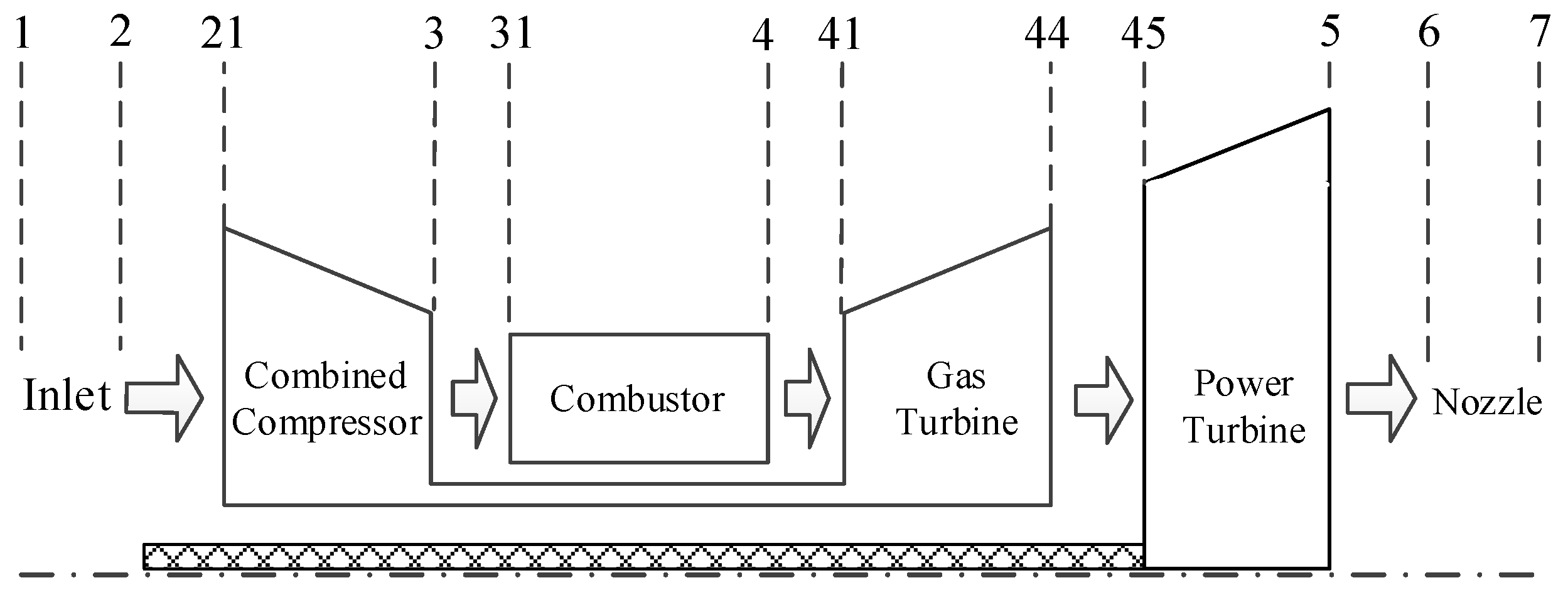
A turboshaft engine can be divided into six typical components, containing an inlet, a combined compressor, a combustor, a gas turbine, a power turbine, and a nozzle. The configuration of the engine is shown in Figure 1, and the definition of each engine section number is listed in Table 1. It is mentioned that the section number is just a label that represents the information of the engine section. Among these components, the rotary components such as the combined compressor, gas turbine, and power turbine must have their own component characteristics. The model for each component is established.
Since the characteristics of aero-engine components at a low-speed state are very difficult to obtain, and the component characteristics provided by R&D departments typically only contain characteristics above idle speed, we must extrapolate the component characteristics to the low-speed state. Currently, a widely used method is to extrapolate the characteristics at low speed from those above idle speed. There are many such extrapolating methods, and here we use the exponential extrapolation method given by Zhou [32]. The results are shown in Figure 2, Figure 3 and Figure 4.
3. Selection of Start-Up Initial Guess Values
3.1. The Manual Method to Select Initial Guess Values
For the ground start-up process of the turboshaft engine, simulations of the initial rotor speed values of its gas turbine rotor and power turbine rotor are both definitely zero. However, to facilitate the calculation and solution process when using one engine model to model the start-up process, small values such as 0.5% or 1% of the designed rotor speed are always chosen as the simulation initial rotor speed values, and generally, the power turbine rotor speed initial value is usually smaller than the power turbine rotor speed initial value . After determining the initial rotor speed values, the problem of selecting initial guess values for the ground start-up simulation of the turboshaft engine has been determining how to find a better set of initial pressure ratio values at the given initial rotor speed values. These initial values should make the engine model converge quickly at the first calculating point while solving the balance equations and ensure the model satisfies the flow balance between each component while ensuring the surplus power of the high-pressure rotor is greater than zero.
At the beginning of the start-up process, the engine inlet air flow rate is very small. If the nozzle exit area is fixed, then the engine inlet air flow rate will be proportional to its total pressure ratio, which is closely related to the pressure ratio or expansion ratio of the rotary components and the total pressure recovery coefficient of each component in the flow channel. Because the engine air flow is very small at the beginning of the start-up process, the wall friction loss is almost negligible when air flows through the flow channel, so a value close to 1 can be taken as the total pressure recovery coefficient of each component when selecting initial guess values. After determining the total pressure recovery coefficient, the total engine air flow rate will be directly determined by the compressor pressure ratio and turbine expansion ratios ,:
The following principles should be followed when choosing the pressure ratio or expansion ratio of rotary components:
- The total pressure ratio of the engine should be above 1.
- The total pressure ratio should be kept constant while adjusting the pressure ratio or expansion ratio of rotary components.
- Selected pressure ratios should ensure interpolation calculation of component characteristics at the given speed line.
- The surplus power of the gas turbine rotor spool calculated by the selected initial pressure values should be greater than zero.
- The rotary components’ inlet flow rate calculated by the selected pressure ratios using component characteristics should meet the flow continuity equations.
- The point interpolated by the selected pressure ratio in the compressor characteristic map should be far from the surge and block boundary.
It is very difficult to simultaneously satisfy the above conditions in the actual debugging process of selecting initial guess values; repeated debugging is needed to obtain a set of initial guess values meeting the equilibrium equation. In some situations, inaccuracy of the component characteristics may lead to the repeated selection of initial guess values such that no point meeting the flow balance can be found, in which case the characteristics must be modified.
The above manual method to select initial guess values, the widely used “cut-and-trail method,” requires a large number of numerical simulations to find a set of initial guess values that push the model to converge quickly. When the type of engine or the environmental conditions of the starting simulation change, the initial guess values usually must be re-selected, which may lead to exhausting repeated work.
3.2. The Flow-Based Back-Calculation Algorithm
3.2.1. Conversion of the Balance Equation
Taking a certain type of turboshaft engine as the modeling object, we will introduce how we use the flow-based back-calculation algorithm to obtain the simulation’s initial guess values. The initial guess values of the turboshaft engine are chosen as follows: Gas turbine rotor speed , power turbine rotor speed , combined compressor pressure ratio, gas turbine expansion ratio, and power turbine expansion ratio.
The balance equations are selected as follows:
(1) Flow rate balance between the combustor outlet section and the gas turbine inlet section:
where represents the flow rate of the combustor outlet section and represents the flow rate of the gas turbine inlet section.
(2) Flow rate balance between the gas turbine outlet section and the power turbine inlet section:
where represents the flow rate of the gas turbine outlet section and represents the flow rate of the power turbine inlet section.
(3) Flow rate balance between the nozzle inlet section and the nozzle outlet section:
where represents the flow rate of the nozzle inlet section and represents the flow rate of the nozzle outlet section.
As can be seen from Formulas (2) to (4), the rotary components and exhaust nozzle of the turboshaft engine are restricted by the principle of flow balance, that is, there are several flow rate balances between them. In the formula above, the flow rates of the gas turbine and power turbine inlet sections can be interpolated and calculated using turbine characteristic maps. For the combustor, the flow rate of its outlet section is determined by the combined compressor, whose flow rate is determined by the compressor characteristic map. As a result, the flow rates of the three rotary components of the turboshaft engine are determined by their corrected speed and pressure ratio.
For the nozzle, its inlet section flow rate is determined by the power turbine outlet section flow rate, while the nozzle outlet section flow rate is determined by its inlet parameters, such as the total pressure , total temperature , environmental static pressure , nozzle outlet area , and air–fuel ratio . At the initial step of the ground start-up process, there is no fuel supply in the combustor, and at the same time, the outlet area of the nozzle and the environmental pressure remain unchanged. Therefore, in the process of calculating initial guess values of the ground start-up process, the calculated flow of the nozzle outlet section is only determined by its inlet parameters and , which can be calculated from the upstream components.
As a result, Formulas (2) to (4) can be converted into the following equation when calculating initial guess values of the ground start-up model:
The initial gas turbine rotor speed and power turbine rotor speed should be given before calculating the initial pressure ratio values. Considering that huge differences in the corrected speed may exist in the rotary component characteristics of different types of aero-engines, and to ensure that each component’s corrected initial-guess speed is larger than the minimum corrected speed characteristics, the initial speed values can be selected by multiplying a given coefficient by the minimum corrected speed of the component characteristic. For the turboshaft engine, the initial high-pressure rotor speed and low-pressure rotor speed can be selected as follows:
where and represent the given proportionality coefficients of the minimum corrected speed lines.
After selecting the initial guess speed values, the problem of selecting initial guess values is converted to an easier problem, which is to find appropriate values of the combined compressor pressure ratio , gas turbine expansion ratio , and power turbine expansion ratio to satisfy the following equation:
3.2.2. Solution Existence Theorem
Figure 2, Figure 3 and Figure 4 show that the rotary component characteristics of one aero-engine have the monotonic feature in the low-speed lines of the start-up process. As can be seen from the monotonic variation of the compressor flow characteristics, in one speed line, the minimum corrected flow of the compressor corresponds to the maximum pressure ratio of the compressor, while the maximum corrected flow of the compressor corresponds to the minimum pressure ratio of the compressor.
Assuming that the initial gas turbine rotor speed corresponds to the corrected speed in the compressor characteristics, in that corrected speed line, we define the maximum corrected flow rate as and the minimum corrected flow rate as . The pressure ratios corresponding to them are defined as and , as shown in Figure 5.
When the compressor corrected flow rate changes from to continuously, the pressure ratio corresponding to it increases from to monotonically and continuously. To satisfy the flow balance, the corrected flow of the gas turbine and the power turbine, which are in the downstream area of the combined compressor, will change from large values and to smaller values and continuously in its corresponding corrected speed line. At the same time, the expansion ratios of the two turbines will also change from large values and to smaller values and continuously in its corresponding corrected speed line. As seen from Figure 3 and Figure 4, the corrected flow of the gas turbine and power turbine has a large span in low corrected speed lines. That means while the corrected flow of the combined compressor changes between the maximum and minimum values, the corrected flow rate of the gas turbine and power turbine only change in an interval, as shown in Figure 6 and Figure 7.
The above analysis has shown that the calculated flow of the nozzle outlet section is only determined by its inlet parameters and . The nozzle inlet total pressure can be determined by the pressure ratio of each rotary component and the total pressure recovery coefficient of each component; since the rotating speed of the start-up process is very low, the total pressure recovery coefficient of each component can be selected as 1, so that can be approximated by the following formula:
When the compressor-corrected flow changes from to continuously, the corresponding pressure ratio increases from to monotonically and continuously. To satisfy the flow balance, the expansion ratios of the gas turbine and power turbine change from large values and to smaller values and continuously in its corresponding corrected speed line. This variation trend of the pressure ratios of the rotary components causes the value of to change from minimum to maximum, which means the inlet total pressure of the nozzle changes from its minimum to its maximum. Because the inlet total pressure of the nozzle determines the calculated flow of the nozzle outlet section, the larger the inlet total pressure, the larger the calculated flow.
From the above analysis, we can draw the following conclusion: In the given corrected speed lines, when the compressor corrected flow changes from its maximum to its minimum continuously and monotonically, the calculated flow of the nozzle outlet section increases from its minimum to its maximum. For the low-speed condition of the ground start-up process, a larger compressor-corrected flow means a larger actual compressor air flow.
In Formulas (2) to (4), there are flow balance relationships between each component and its adjacent components, and therefore, implicit flow balance relationships exist between each pair of adjacent components of the aero-engine. An important implicit relationship is that flow balance exists between the flow of the compressor outlet section and that of the nozzle outlet section.
Thus, one important conclusion is the following: With the given initial guess speed values, if the compressor flow range calculated by the compressor flow characteristic intersects with the range of the calculated flow of the nozzle outlet section, then a set of initial guess pressure ratios making each component satisfy flow balance can certainly be solved with the given initial guess speed values. If no intersection exists, then no set of initial guess pressure ratios making each component satisfy flow balance can be solved with the given initial guess speed values, which means the component characteristics must be amended.
3.2.3. Solution of Initial Guess Values
The sections below will clarify the specific process of solving the initial pressure ratios with the existence of a solution.
Figure 8 shows six cases in which there is an intersection between the compressor-corrected flow range and the range of the calculated flow of the nozzle outlet section. The calculated flow of the nozzle outlet section has been corrected, and the span of the intersection is determined by the rotary component characteristics in Figure 8.
The corrected flow of the compressor must be in the intersection of the two flows in Figure 8 when each component satisfies the flow balance. The lower and upper limits of the intersection can be obtained by the following formula:
where the maximum and minimum values of the corrected flow and pressure ratio of the compressor can be calculated by the following formula:
The calculating process of the maximum and minimum values of the nozzle flow is as follows. We take the result of the minimum compressor pressure ratio and the maximum compressor pressure ratio as the initial values of the compressor pressure ratio and perform the regular flow path calculations. Then, the mass flow of the downstream gas turbine inlet section will be solved, converting the mass flow to corrected flow and using the inverse interpolation function to interpolate the expansion ratio of the gas turbine:
We take the result of the expansion ratio as the initial value of the gas turbine expansion ratio and perform the flow path calculation of the gas turbine. Then, the mass flow of the downstream power turbine inlet section can be solved, converting it to a corrected flow and using it to interpolate the expansion ratio of the power turbine:
We take the result of the expansion ratio as the initial value of the power turbine expansion ratio and perform the flow path calculation of the gas turbine. Then, the inlet parameters of the downstream nozzle can be solved and used to solve the calculated flow of the nozzle outlet section:
Through the process above, using the minimum compressor pressure ratio calculated by Formula (10) can solve the minimum calculated flow of the nozzle outlet section while using the maximum compressor pressure ratio calculated by Formula (10) can solve the maximum calculated flow of the nozzle outlet section.
In the calculation process above, the flow balance between the combustor and the gas turbine and between the power turbine and the gas turbine are both guaranteed, which means the balance Equations (2) and (3) are already established. Because the expansion ratios of the gas turbine and the power turbine can be solved by inverse interpolation, one nozzle flow can be solved with one compressor pressure ratio, so the balance equation represented by Formula (7) can be converted into the following formula:
The difficult problem of selecting the initial guess values is now simplified to the problem of searching for an initial compressor pressure ratio to enable us to use Formula (14) to represent the balance equation.
For the situation shown in Figure 8b,f, the minimum calculated flow of the nozzle is negative, indicating that the total pressure ratio of the aero-engine is less than 1 when the compressor flow changes from its maximum to its minimum, which will result in nozzle inverse flow. This situation must be restricted to improve the degree of closeness between the real initial guess values and the “fake initial values” calculated.
According to the above process of solving the nozzle flow, the expansion ratio of the gas turbine and the expansion ratio of the power turbine can be solved through inverse interpolation by the pressure ratio of the compressor based on flow balance. When the compressor flow changes from its maximum to its minimum, the pressure ratio of the compressor gradually increases; however, the expansion ratios of the gas turbine and the power turbine gradually decrease based on the analysis above. The total pressure ratio of the aero-engine is approximately , so the total pressure ratio of the aero-engine gradually increases when the compressor flow changes from its maximum to its minimum. Thus, the situation in which the minimum calculated flow of the nozzle is negative, as shown in Figure 8b,f, only occurs when the compressor flow is near its maximum. The interval between the maximum and minimum flow of the compressor can be divided into equal parts and changes according to the requirement of precision. is 100 in this article. By gradually decreasing the compressor flow from the maximum flow and making use of the inverse interpolation function, the compressor pressure ratio corresponding to the flow can be solved, and then the expansion ratios of the gas turbine and power turbine can be calculated using Formulas (11) and (12). We perform the above calculation process until the total pressure ratio of the aero-engine is greater than 1, and we replace the flow with the compressor flow in Formula (9) to solve a new upper limit flow .
We take the flow midway between the lower and upper limits of the intersection of the compressor flow and the nozzle flow as :
In the compressor characteristics, the pressure ratio of the compressor can be solved with the inverse interpolation of . With the help of Formulas (11) and (12), the expansion ratio of the gas turbine and the expansion ratio of the power turbine can both be solved. , , and are the so-called “fake initial values.”
For the situation shown in Figure 8e, the upper and lower limits of the intersection solved are the maximum and minimum compressor flows at the given corrected speed line, which to some extent affects the accuracy of the “fake initial values” and conflicts with the later iterative solution of the real initial guess values.
According to the above analysis, when the compressor flow changes from its maximum to its minimum, the pressure ratio of the compressor increases gradually, and the total pressure ratio of the aero-engine also increases gradually, which finally contributes to the gradual increase in the calculated flow of the nozzle outlet section. The interval between the maximum and minimum compressor pressure ratios can be divided into equal parts and changes according to the requirement of precision. In this article, is selected as 100. We gradually increase the compressor pressure ratio from the minimum to the maximum and calculate the nozzle flow using Formulas (11) to (13) until the calculated flow of the nozzle is larger than the minimum compressor flow. Defining the compressor pressure ratio previously as , its corresponding flow is . Replacing the flow with in Formula (9), we can solve the new upper limit flow . Then, we can solve a new set of “fake initial values”, which include , , and , using Formulas (15), (11), and (12). The narrowing of the intersection of the flow brings the “fake initial values” closer to the real initial guess values.
Similarly, the new lower limit flow can be calculated by way of calculating the maximum compressor pressure ratio and can further improve the accuracy of the “fake initial values.”
The Newton iteration method is a powerful mathematical method for the equation approximation solution in fields of real numbers and complex numbers. It has been widely applied to diverse fields, such as the simulation of industrial equipment [33], the parameter identification of transfer functions [34], and the design of basic science [35]. In addition, the improvement of the Newton iteration method constitutes challenging and meaningful research to enhance the global convergence capability [36,37,38]. When the Jacobian matrix is positively definite and the initial values are close to the real initial guess values, the Newton iterative method has second-order convergence. Taking advantage of the convergence of the Newton iterative method, the real initial guess values can be solved by taking the “fake initial values” obtained above as the initial point of the iterative solution. The above traversal calculation of the flow has narrowed the intersection of the compressor flow and the nozzle flow, which makes the “fake initial values” much closer to the real initial guess values and ensures the true values of the initial guess values can be solved by iteration.
In the process of iteratively solving for the true initial guess values, we have added the restriction that the surplus power of the gas turbine is greater than zero. So, the pressure ratios , , and can finally be solved. , , , and the speeds and defined by Formula (6) are called the ground initial guess values that can make the model converge.
3.3. Expansion of the Flow-Based Back-Calculation Algorithm
The idea of our proposed FBBCA can also be applied to other types of component-level aero-engine models to select the initial guess values.
The following will take the twin-shaft mixed exhaust turbofan engine as an example to show how the FBBCA can be expanded to other types of component-level aero-engine models.
Figure 9 is the functional block diagram of a twin-shaft mixed exhaust turbofan engine.
3.3.1. Conversion of the Balance Equation
The initial guess values of the twin-shaft mixed exhaust turbofan engine are chosen as follows: High-pressure rotor speed , low-pressure rotor speed , fan blade tip pressure ratio , compressor pressure ratio , high-pressure turbine expansion ratio , and low-pressure turbine expansion ratio .
The balance equations are selected as follows:
(1) Flow balance between the combustor outlet section and the high-pressure turbine inlet section:
where represents the flow of the combustor outlet section and represents the flow of the high-pressure turbine inlet section.
(2) Flow balance between the high-pressure turbine outlet section and the low-pressure turbine inlet section:
where represents the flow of the high-pressure turbine outlet section and represents the flow of the low-pressure turbine inlet section.
(3) Flow balance between the nozzle inlet section and the nozzle outlet section:
where represents the flow of the nozzle inlet section and represents the flow of the nozzle outlet section.
(4) Static pressure balance between the low-pressure turbine outlet section and the bypass outlet section:
where represents the static pressure of the low-pressure turbine outlet section and represents the static pressure of the bypass outlet section.
Formula (19) ensures the flow balance between the fan blade root outlet section and the compressor inlet section. From the above analysis of Formulas (2) to (4), we can convert Formulas (16) to (19) to the following equation when calculating initial guess values of a ground start:
According to the analysis of the turboshaft engine, the expansion ratio of the high-pressure turbine and low-pressure turbine downstream of the compressor can be calculated by the compressor ratio through the flow balance. Because Formula (19) ensures the flow balance between the fan and the compressor, the fan blade root ratio can also be calculated by the compressor ratio. An important implicit relationship can be achieved from Formulas (16) to (19), which is that flow balance exists between the flow of the fan outlet section and the flow of the nozzle outlet section.
Thus, one important conclusion is the following: With the given initial-guess speed values, if the fan flow range calculated by the fan flow characteristic intersects with the range of the calculated flow of the nozzle outlet section, then a set of initial-guess pressure ratios that causes each component to satisfy the flow balance can certainly be solved with the given initial guess speed values. If no intersection exists, then no set of initial-guess pressure ratios making each component satisfy the flow balance can be solved with the given initial-guess speed values, which means the component characteristics must be amended.
3.3.2. Solution of Initial Guess Values
For the condition of existing solutions, the process of solving the initial guess values is as follows:
As with the turboshaft engine, we can select the high-pressure rotor speed and low-pressure rotor speed according to Formula (6). There are two compression components in the twin-shaft mixed exhaust turbofan engine—the fan and the compressor—and the compressor is more likely to enter the surge and blocking state. Therefore, it is wise to take the compressor as the center to calculate the initial pressure ratios of the twin-shaft mixed exhaust turbofan engine.
To solve the corrected speed corresponding to the initial speed value of the compressor and the maximum corrected flow, the minimum corrected flow, the maximum pressure ratio, and the minimum pressure ratio in this corrected speed line, we must determine the inlet parameters of the compressor. However, the outlet parameters of the upstream fan are unknown, which makes the inlet parameters of the compressor unsolvable. Considering that the pressure ratios of compression components are very close to 1, the fan may encounter static in the initial stage of start-up, which means the fan is doing no work to the air flowing through it. So, it is reasonable to assume the pressure ratio of the fan is 1 to calculate the inlet parameters of the downstream compressor. With the parameters solved, the corrected speed can be solved, and then we can use Formula (10) to solve the maximum corrected flow, minimum corrected flow, maximum pressure ratio, and minimum pressure ratio in this corrected speed line.
By taking the result of the minimum compressor pressure ratio and the maximum compressor pressure ratio , respectively, as the initial value of the compressor pressure ratio, we can solve the outlet parameters and the expansion ratio of the low-pressure turbine by using Formulas (11) and (12). The compressor inlet flow can be solved by interpolation, and due to the flow balance between the fan blade root outlet and the compressor inlet, the fan blade root outlet flow equals . Because there is no bleed air in the fan, the fan blade root inlet flow is . Using the inverse interpolation function, the fan blade root pressure ratio can be solved. Then, using Formula (21), the pressure ratio and flow of the fan blade tip can be solved:
After solving the flow of the fan blade root and fan blade tip, the outlet flow of the fan can be solved. According to the flow balance between the fan blade root and the compressor, it is clear that by using the minimum pressure ratio as the initial pressure ratio of the compressor, we can solve the maximum flow of the fan, and we can use the maximum pressure ratio as the initial pressure ratio to solve the minimum flow of the fan. Using the parameters obtained by Formula (21), the outlet parameters of the fan can all be solved, and these can be used to calculate the inlet parameters of the bypass. Performing the flow path calculation of the bypass, the outlet parameters of the bypass can also be solved.
Knowing the outlet parameters of the bypass and the low-pressure turbine, the flow path calculation of the mixer can be performed to solve the inlet parameters of the downstream nozzle, as Formula (13) shows. From the above analysis of the turboshaft engine, we know that by using the minimum pressure ratio of the compressor, the minimum fan pressure ratio, the maximum high-pressure turbine expansion ratio, and the maximum high-pressure turbine expansion ratio can be solved, so the nozzle flow that is solved is the minimum. In a word, the minimum compressor ratio represents the maximum fan flow and the minimum nozzle flow , while the maximum compressor ratio represents the minimum fan flow and the maximum nozzle flow .
In the calculation process above, the flow balance between the fan blade root and the compressor, the flow balance between the high-pressure turbine and the combustor, and the flow balance between the low-pressure turbine and the high-pressure turbine are all guaranteed. The fan pressure ratio, the high-pressure turbine expansion ratio, and the low-pressure turbine expansion ratio all can be solved by inverse interpolation of the flow. So, using one compressor pressure ratio can solve one nozzle flow, and we can convert Formula (20) to the form of Formula (14).
The subsequent calculation process is the same as Formula (15). After solving the middle flow and using the inverse interpolation function to solve the compressor pressure ratio , we can solve the fan blade tip pressure ratio , the high-pressure turbine expansion ratio , and the low-pressure turbine expansion ratio with the help of Formulas (21), (11), and (12). , , , and are the so-called “fake initial values.” Then, using Newton’s method, we can obtain the true initial guess values.
For the twin-shaft turbojet engine similar to the twin-shaft mixed-exhaust turbofan engine, the initial guess values can be solved by the same theory used to solve the pressure ratio of the low-pressure compressor. For the single-shaft aero-engine, the initial guess values can be solved by the FBBCA by simplifying the calculating process of the turboshaft engine. So, the method proposed by this article can be applied to other types of component-level aero-engine models to select initial guess values. An illustration of the selection of start-up initial guess values is presented in Figure 10.
4. Simulation
4.1. Simulation under Different Speeds
Taking a certain type of turboshaft engine as an example, we select different proportionality coefficients according to Formula (6). Using different initial guess speed values to calculate the start-up initial guess values with the iteration tolerance set to 0.001, the ambient pressure set to 101,325 Pa, and the ambient temperature set to 288.15°K, the input of the given initial guess speed values and the corresponding simulation results are shown in Figure 11 and Figure 12, respectively.
With the same initial-guess speed and environmental parameters, the simulation results with the iteration tolerance set to 0.005 are shown in Figure 13.
Figure 11, Figure 12 and Figure 13 show that, even when the variation range of the given initial speed values is very large, initial guess values that make the model converge can still be solved with the algorithm presented in this article. By comparing the solved pressure ratios in Figure 12 and Figure 13, we can obtain the following conclusions. Reducing the iteration tolerance appropriately can significantly reduce the NR iteration number while the solved pressure ratios only change slightly, as shown by the fact that the error between the solved pressure ratios in Figure 12 and Figure 13 at the same speed is less than 1‰. Such a tiny error also shows that tiny variations of pressure ratios can contribute to large variations of flow error at low speed, and if using the artificial method to select initial guess values, the difficulty and workload will be enormous.
4.2. Simulation under Different Environmental Conditions
China’s vast territory and large latitude and longitude values lead to a large span of temperatures. The maximum temperature in China can be as high as 320.15°K, while the minimum temperature can be as low as 221.15°K. The lowest altitude of major cities is near sea level, with atmospheric pressure close to standard atmospheric pressure, and the highest altitude is up to 4 km, with atmospheric pressure as low as 64,000 Pa. Accordingly, aircraft engines in China can face a variety of starting environmental conditions, including plateaus, alpine conditions, high temperatures, and other extreme conditions. This section will select typical sample points in the range of environmental parameters in China to verify the adaptability of the FBBCA.
Taking a turboshaft engine as an example and changing the environmental parameters at the same initial guess speed ( and ), the input of the environmental parameters and the corresponding simulation results are shown in Figure 14 and Figure 15, respectively.
At the given initial guess speed, the convergence of 441 points of initial guess values calculated by the FBBCA in this turboshaft engine’s environmental envelope is shown in Figure 16.
Figure 15 shows that the atmospheric temperature has a large impact on the initial guess values, while the atmospheric pressure has negligible impacts. Figure 16 shows that the algorithm presented in this article can always solve suitable initial guess values, making the model converge in response to the changing environmental parameters. The algorithm has self-adaptability.
Furthermore, turboshaft engine performance comparisons at complete start-up conditions between a real engine and the component-level model are shown in Figure 17. The experiment was measured in a rig test. As shown in Figure 17, the simulation curves are essentially consistent with the experimental curves.
4.3. Simulation with Different Types of Aero-Engines
This section will take two types of single-shaft turbojet engines and a twin-shaft turbofan engine as examples to verify the universality of the FBBCA proposed by this paper.
The simulation results of type A and type B single-shaft turbojet engines using the FBBCA under different environmental conditions are shown in Table 2.
Table 2 shows that the FBBCA proposed by this article can be applied to different types of aero-engines and solve their relevant initial guess values. At the same time, the algorithm can adjust the initial guess speed automatically according to the component characteristics and solve the corresponding initial guess pressure ratios. In addition to this, the algorithm can adjust the solved initial guess values automatically according to the variation of the environment to ensure the model always converges.
Taking the twin-shaft turbofan engine as an example to verify the universality of the FBBCA, the input of the environmental parameters and the corresponding simulation results are shown in Figure 18 and Figure 19, respectively.
Figure 19 shows that for the twin-shaft turbofan engine, the algorithm can solve its ground initial guess values quickly and accurately. As can be seen in Figure 19, when the low-pressure rotor initial guess value is very small, the fan pressure ratio solved is below 1, which is consistent with the theoretical analysis. When the fan speed is very low, the work performed on the airflow by the fan is nearly zero. However, when air flows through the fan, a total pressure loss will be generated, which will make the pressure ratio of the fan less than 1, which is why fan pressure ratios less than 1 can be observed in Figure 19. The literature also mentions that at a very low-speed state, the pressure of the fan tip outlet or bypass inlet might be lower than the environmental pressure, which will contribute to the backward flow of the bypass nozzle [25]. This also verifies the rationality of the FBBCA proposed in this article. When the fan speed increases, the power provided by the fan increases and the total power is greater than the loss, which will make the pressure ratio of the fan greater than 1, as shown in the fourth group in Figure 19.
4.4. Comparison of the Manual Method and the Flow-Based Back-Calculation Algorithm
Compared with the manual method, the FBBCA proposed by this paper has the following advantages:
1. The FBBCA can quickly calculate the initial guess values of a component-level aero-engine start-up model in only a few seconds, while the traditional manual method usually takes several hours or even several days to select an appropriate set of initial guess values that can make the model converge. For example, for the type of turboshaft engine discussed above, the manual “cut-and-trail method” took half a day to select a set of initial guess values that made the model converge. When the structure of the engine is more complex, such as the twin-shaft mixed-exhaust turbofan engine, the manual “cut-and-trail method” will consume much more time. A survey in research institutions indicates that the traditional manual “cut-and-trail method” for the selection of initial guess values of a twin-shaft engine could take one or two days. It is extremely dependent on the designers’ experience and the reliability of the low-speed component characteristics. The manual method for zero-based researchers could consume over a week. To avoid such a circumstance, for the same engine configuration, some researchers could copy low-speed component characteristics and corresponding initial guess values from one designed engine to another undesigned engine. However, this approach can obviously reduce the confidence of the aero-engine at start-up conditions.
2. The FBBCA can quickly judge whether the initial guess values have a solution and show the scope of the solution based on the component characteristics.
Extrapolating the component characteristics in a low-speed state from its characteristics above idle speed cannot ensure the accuracy of the extrapolated characteristics. This extrapolation might sometimes even cause a mismatch problem between the components’ characteristics, leading to no solution for the initial guess values. However, the selection of initial guess values assumes that the model has a solution, and no one knows whether the model does have a solution. In the case where no solution exists, the manual “cut-and-trail method” attributes the divergence of the start-up model to the wrong selection of the initial guess values, and more time will be taken to repeatedly select new initial guess values until the mismatching problem of component characteristics has been identified. However, much time and energy have already been wasted.
The FBBCA proposed by this paper can quickly judge whether the initial guess values have a solution, show the scope of the solution based on the component characteristics, and avoid the case of no solution that can be encountered by the manual “cut-and-trail method.” Figure 20 shows the solution scope in the combined compressor flow characteristic of the type of turboshaft engine discussed above.
As can be seen from Figure 20, the solution scope only accounts for a small part of the overall flow characteristics, which also reflects the difficulty of using the manual “cut-and-trail method” to select the initial guess values. Figure 21 shows that the final convergent point of the model is strictly in the solution scope, which proves the reliability and rationality of the FBBCA. If no solution scope can be solved by the FBBCA, the component characteristics have a mismatching problem that must be corrected. Due to this, the large amount of time and energy wasted by the manual method can be avoided.
3. The FBBCA has good generality and self-adaptability. The initial guess values obtained by the traditional manual method are only for a certain type of aero-engine. A change in either the engine type or version will result in the initial guess values being no longer applicable, and then the initial guess values must be re-selected. In addition, if the initial guess speeds change, the corresponding initial guess pressure ratios obtained by the manual method might make it difficult for the model to converge, and even might result in the divergence of the model. Table 3 shows the variation of the NR iteration number of the initial guess values obtained by both the manual method and the FBBCA for the type of turboshaft engine discussed above. The iteration tolerance is set to 0.001, the ambient pressure is set to 101,325 Pa, and the ambient temperature is set to 288.15°K. For the manual “cut-and-trail method,” the initial guesses of the gas turbine rotor speed and power turbine rotor speed are 30 rpm and 20 rpm, respectively.
It can be seen from Table 3 that the initial guess values selected by the manual “cut-and-trail method” can only make the model converge quickly at the corresponding initial-guess speeds. When the initial-guess speeds change, the NR iteration number greatly increases. However, the FBBCA proposed by this paper can make the model converge quickly at any given initial-guess speed. In addition, the initial guesses of the pressure ratios of the turboshaft engine, in this case, are only 3; when the engine type becomes more complex, the initial guesses of pressure ratios might increase to 4, or even 5. By that time, it is difficult for the initial guess values obtained by the manual method to guarantee that the model still converges when the initial-guess speeds change greatly.
In summary, the FBBCA proposed by this article can solve the initial guess values of a component-level aero-engine model quickly and accurately and can be adapted to the variation of environmental parameters and multiple types of engine models.
5. Conclusions
In this paper, a novel generation method for initial guess values was introduced that aimed to adaptively achieve initial guess values of the aero-engine component-level models at the start-up condition. The relevant verifications are as follows:
(1) The FBBCA proposed by this article has good universality and can be applied to solve the initial guess values of ground start-up models for the main types of aero-engines, such as turbojet, turboshaft, and turbofan engines.
(2) The FBBCA can solve the initial guess values at a given corrected speed quickly and accurately. This algorithm can adapt to changes in environmental parameters automatically to ensure the initial guess values always result in convergence.
(3) The FBBCA can simplify the work of selecting initial guess values and save a large amount of numerical simulation work required by the “cut-and-trail method”, so this method has practical significance.
Author Contributions
Conceptualization, W.Z.; methodology, W.K. and S.L.; software, W.K. and S.L.; validation, W.Z. and F.L.; formal analysis, S.L.; investigation, W.Z. and F.L.; resources, J.W. and C.Z.; data curation, S.L.; writing—original draft preparation, S.L. and W.K.; writing—review and editing, W.Z. and F.L.; visualization, W.Z.; supervision, J.W. and C.Z.; project administration, W.Z. and C.Z.; funding acquisition, W.Z. and J.W. All authors have read and agreed to the published version of the manuscript.
Funding
This research was co-funded by the National Science and Technology Major Project (No. J2019-I-0010-0010).
Institutional Review Board Statement
Not applicable.
Informed Consent Statement
Not applicable.
Data Availability Statement
Data are contained within the article.
Acknowledgments
The authors gratefully acknowledge the financial support for this project from the National Science and Technology Major Project (No. J2019-I-0010-0010).
Conflicts of Interest
The authors declare that they have no known competing financial interests or personal relationships that could have appeared to influence the work reported in this paper.
Nomenclature
| engine flow | |
| expansion ratio | |
| flow-based back-calculation algorithm | |
| rotor speed, rpm | |
| pressure, Pa | |
| environmental pressure | |
| pressure ratio | |
| temperature, K | |
| total pressure | |
| mass flow rate | |
| pressure ratio/expansion ratio | |
| Subscripts | |
| air | |
| corrected parameter | |
| compressor | |
| fan | |
| fan blade tip | |
| fan blade root | |
| gas | |
| gas turbine rotor | |
| gas turbine | |
| high-pressure rotor | |
| high-pressure turbine | |
| low-pressure rotor | |
| low-pressure turbine | |
| nozzle | |
| power turbine rotor | |
| power turbine | |
| static | |
| total | |
| 1–9 | engine interface symbols |
References
- Topel, M.; Nilsson, Å.; Jöcker, M.; Laumert, B. Investigation into the thermal limitations of steam turbines during start-up operation. J. Eng. Gas Turbines Power 2018, 140, 012603. [Google Scholar] [CrossRef]
- Guan, J.; Lv, X.; Spataru, C.; Weng, Y. Experimental and numerical study on self-sustaining performance of a 30-kW micro gas turbine generator system during startup process. Energy 2021, 236, 121468. [Google Scholar] [CrossRef]
- Sheng, H.; Chen, Q.; Li, J.; Jiang, W.; Wang, Z.; Liu, Z.; Zhang, T.; Liu, Y. Research on dynamic modeling and performance analysis of helicopter turboshaft engine’s start-up process. Aerosp. Sci. Technol. 2020, 106, 106097. [Google Scholar] [CrossRef]
- Rossi, I.; Sorce, A.; Traverso, A. Gas turbine combined cycle start-up and stress evaluation: A simplified dynamic approach. Appl. Energy 2017, 190, 880–890. [Google Scholar] [CrossRef]
- Nannarone, A.; Klein, S.A. Start-Up Optimization of a CCGT Power Station Using Model-Based Gas Turbine Control. J. Eng. Gas Turbines Power 2019, 141, 041018. [Google Scholar] [CrossRef]
- Jafari, S.; Miran Fashandi, S.A.; Nikolaidis, T. Modeling and control of the starter motor and start-up phase for gas turbines. Electronics 2019, 8, 363. [Google Scholar] [CrossRef]
- Qin, H.; Zhao, J.; Ren, L.; Li, B.; Li, Z. Performance Degradation Evaluation of Low Bypass Ratio Turbofan Engine Based on Flight Data. Sustainability 2022, 14, 8052. [Google Scholar] [CrossRef]
- Ren, L.; Qin, H.; Xie, Z.; Xie, J.; Li, B. A Thermodynamics-Oriented and Neural Network-Based Hybrid Model for Military Turbofan Engines. Sustainability 2022, 14, 6373. [Google Scholar] [CrossRef]
- Ying, Y.; Cao, Y.; Li, S.; Li, J. Nonlinear steady-state model based gas turbine health status estimation approach with improved particle swarm optimization algorithm. Math. Probl. Eng. 2015, 2015, 940757. [Google Scholar] [CrossRef]
- Park, Y.; Choi, M.; Choi, G. Fault detection of industrial large-scale gas turbine for fuel distribution characteristics in start-up procedure using artificial neural network method. Energy 2022, 251, 123877. [Google Scholar] [CrossRef]
- Fentaye, A.D.; Gilani, S.I.U.H.; Baheta, A.T. Gas turbine gas path diagnostics: A review. MATEC Web Conf. 2016, 74, 00005. [Google Scholar] [CrossRef]
- Erario, M.L.; De Giorgi, M.G.; Przysowa, R. Model-Based Dynamic Performance Simulation of a Microturbine Using Flight Test Data. Aerospace 2022, 9, 60. [Google Scholar] [CrossRef]
- Qian, Y.; Ye, Z.; Zhang, H. Impact of Modeling Simplifications on Lightning Strike Simulation for Aeroengine. Math. Probl. Eng. 2019, 2019, 5176560. [Google Scholar] [CrossRef]
- Asgari, H.; Chen, X.Q.; Morini, M.; Pinelli, M.; Sainudiin, R.; Spina, P.R.; Venturini, M. NARX models for simulation of the start-up operation of a single-shaft gas turbine. Appl. Therm. Eng. 2016, 93, 368–376. [Google Scholar] [CrossRef]
- Ghaffari, A.; Akhgari, R.; Abbasi, E. Modeling and Simulation of MGT-70 Gas Turbine start-up procedure. Amirkabir J. Mech. Eng. 2017, 49, 363–370. [Google Scholar]
- Agrawal, R.K. A Generalized Mathematical Model to Estimate Gas Turbine Starting Characteristics ASME Paper. In Turbo Expo: Power for Land, Sea, and Air; American Society of Mechanical Engineers: New York, NY, USA, 1980; No. 81-GT-202. [Google Scholar]
- Davis, J.B.; Pollak, R.R. Criteria for Optimizing Starting Cycles for High Performance Fighter Engines. In Proceedings of the 19th Joint Propulsion Conference, Seattle, WA, USA, 27–29 June 1983. AIAA-83-1127. [Google Scholar]
- Chappell, M.A.; McLaughlin, P.W. Approach to Modeling Continuous Turbine Engine Operation from Startup to Shutdown. J. Propuls. Power 1993, 9, 466–471. [Google Scholar] [CrossRef]
- Braig, W.; Schulte, H.; Riegler, C. Comparative Analysis of the Windmilling Performance of Turbojet and Turbofan Engines. J. Propuls. Power 1999, 15, 326–333. [Google Scholar] [CrossRef]
- Owen, A.K.; Daugherty, A.; Garrard, D.; Reynolds, H.C.; Wright, R.D. A Parametric Starting Study of an Axial-Centrifugal Gas Turbine Engine Using a One-Dimensional Dynamic Engine Model and Comparisons to Experimental Results: Part I—Model Development and Facility Description. J. Eng. Gas Turbines Power 1999, 121, 377–383. [Google Scholar] [CrossRef]
- Owen, A.K.; Daugherty, A.; Garrard, D.; Reynolds, H.C.; Wright, R.D. A Parametric Starting Study of an Axial-Centrifugal Gas Turbine Engine Using a One-Dimensional Dynamic Engine Model and Comparisons to Experimental Results: Part II—Simulation Calibration and Trade-Off Study. J. Eng. Gas Turbines Power 1999, 121, 384–393. [Google Scholar] [CrossRef]
- Kim, J.H.; Song, T.W. Dynamic Simulation of Full Startup Procedure of Heavy-Duty Gas Turbines. J. Eng. Gas Turbines Power 2002, 124, 510–516. [Google Scholar] [CrossRef]
- Riegler, C.; Bauer, M.; Schulte, H. Validation of a Mixed Flow Turbofan Performance Model in the Sub-Idle Operating Range. In Turbo Expo: Power for Land, Sea, and Air; American Society of Mechanical Engineers: New York, NY, USA, 2003; GT2003-38223. [Google Scholar]
- Pakanati, S.; Sampath, R.; Irani, R.; Plybon, R.; Anderson, B. High Fidelity Engine Performance Models for Windmill Relight Predictions. In Proceedings of the Joint Propulsion Conference & Exhibit, Sacramento, CA, USA, 9–12 July 2006. AIAA 2006-4970. [Google Scholar]
- Bretschneider, S.; Reed, J. Modeling of Start-Up from Engine-Off Conditions Using High Fidelity Turbofan Engine Simulations. J. Eng. Gas Turbines Power 2016, 138, 051201-1–051201-6. [Google Scholar] [CrossRef]
- Asgari, H.; Chen, X.; Sainudiin, R.; Morini, M.; Pinelli, M.; Spina, P.R.; Venturini, M. Modeling and simulation of the start-up operation of a heavy-duty gas turbine by using NARX models. In Turbo Expo: Power for Land, Sea, and Air; American Society of Mechanical Engineers: New York, NY, USA, 2014; Volume 45653, p. V03AT21A003. [Google Scholar]
- Mehrpanahi, A.; Hamidavi, A.; Ghorbanifar, A. A novel dynamic modeling of an industrial gas turbine using condition monitoring data. Appl. Therm. Eng. 2018, 143, 507–520. [Google Scholar] [CrossRef]
- Bahlawan, H.; Morini, M.; Pinelli, M.; Spina, P.R.; Venturini, M. Development of reliable narx models of gas turbine cold, warm and hot start-up. In Turbo Expo: Power for Land, Sea, and Air; American Society of Mechanical Engineers: New York, NY, USA; Charlotte, NC, USA, 2017; Volume 50961, p. V009T27A007. [Google Scholar]
- Mathioudakis, K.; Politis, E.; Stamatis, A. A computer model as an educational tool for gas turbine performance. Int. J. Mech. Eng. Educ. 1999, 27, 114–125. [Google Scholar] [CrossRef]
- Flack, R.D. Analysis and Matching of Gas Turbine Components. Int. J. Turbo Jet Engines 1990, 7, 217–226. [Google Scholar] [CrossRef]
- Zhou, W.X. Research on Object-Oriented Modeling and Simulation for Aeroengine and Control System. Ph.D. Thesis, Nanjing University of Aeronautics and Astronautics, Nanjing, China, 2006. (In Chinese). [Google Scholar]
- Zhou, W.X.; Huang, J.Q. Development of Component-Level Startup Model for a Turbofan Engine. J. Aerosp. Power 2006, 21, 248–253. (In Chinese) [Google Scholar]
- Wu, Y.; Liu, B.; Zhang, H.; Zhu, K.; Kong, B.; Guo, J.; Li, F. Accuracy and efficient solution of helical coiled once-through steam generator model using JFNK method. Ann. Nucl. Energy 2021, 159, 108290. [Google Scholar] [CrossRef]
- Wang, C.; Yu, H.; Wang, J.; Liu, T. Bias analysis of parameter estimator based on Gauss-Newton method applied to ultra-wideband positioning. Appl. Sci. 2019, 10, 273. [Google Scholar] [CrossRef]
- Failer, L.; Richter, T. A parallel Newton multigrid framework for monolithic fluid-structure interactions. J. Sci. Comput. 2020, 82, 28. [Google Scholar] [CrossRef]
- Klemetsdal, Ø.; Moncorgé, A.; Møyner, O.; Lie, K.A. A numerical study of the additive Schwarz preconditioned exact Newton method (ASPEN) as a nonlinear preconditioner for immiscible and compositional porous media flow. Comput. Geosci. 2022, 26, 1045–1063. [Google Scholar] [CrossRef]
- Xu, P.; Roosta, F.; Mahoney, M.W. Newton-type methods for non-convex optimization under inexact Hessian information. Math. Program. 2020, 184, 35–70. [Google Scholar] [CrossRef]
- Yuan, G.; Sheng, Z.; Wang, B.; Hu, W.; Li, C. The global convergence of a modified BFGS method for nonconvex functions. J. Comput. Appl. Math. 2018, 327, 274–294. [Google Scholar] [CrossRef]
Figure 1.
Functional block diagram of turboshaft engine.

Figure 2.
Functional block diagram of turboshaft engine.

Figure 3.
Gas turbine inlet gas flow rate characteristics.

Figure 4.
Power turbine inlet gas flow rate characteristics.

Figure 5.
Single speed line of compressor flow rate characteristic.

Figure 6.
Single speed line of gas turbine flow characteristic.

Figure 7.
Single speed line of power turbine flow characteristic.

Figure 8.
Intersection situations of compressor and nozzle.

Figure 9.
Functional block diagram of twin-shaft mixed exhaust turbofan engine.

Figure 10.
Illustration of the selection of start-up initial guess values.

Figure 11.
Input of given initial guess speed values with iteration tolerance set to 0.001.

Figure 12.
Simulation of start-up initial guess values with iteration tolerance set to 0.001.

Figure 13.
Simulation of start-up initial guess values with iteration tolerance set to 0.005.

Figure 14.
Input of different environmental conditions.

Figure 15.
Simulation under different environmental conditions with iteration tolerance set to 0.001.
Figure 15.
Simulation under different environmental conditions with iteration tolerance set to 0.001.

Figure 16.
Convergence of initial guess values in the environmental envelope.

Figure 17.
Comparisons between experimental data and model simulation data.

Figure 18.
Input of the environmental parameters of a twin-shaft turbofan aero-engine.

Figure 19.
Simulation results of a twin-shaft turbofan aero-engine with iteration tolerance set to 0.001.
Figure 19.
Simulation results of a twin-shaft turbofan aero-engine with iteration tolerance set to 0.001.

Figure 20.
Solution scope in compressor flow characteristic of the turboshaft engine.

Figure 21.
Zoom of the solution scope.


Table 1.
Definition of engine section numbers.
| Section Number | Definition | Section Number | Definition |
|---|---|---|---|
| 1 | Inlet inlet | 41 | Gas turbine inlet |
| 2 | Inlet outlet | 44 | Gas turbine outlet |
| 21 | Combined compressor inlet | 45 | Power turbine inlet |
| 3 | Combined compressor outlet | 5 | Power turbine outlet |
| 31 | Combustor inlet | 6 | Nozzle inlet |
| 4 | Combustor outlet | 7 | Nozzle outlet |
Table 2.
Simulation results of two types of single-shaft turbojet aero-engines with iteration tolerance set to 0.001.
Table 2.
Simulation results of two types of single-shaft turbojet aero-engines with iteration tolerance set to 0.001.
| Type A | Type B | |||||
|---|---|---|---|---|---|---|
| 101,325 Pa, 288.15°K | 190.7 | 1.006376 | 1.006231 | 202.8 | 1.004524 | 1.003424 |
| 101,325 Pa, 313.15°K | 190.7 | 1.006227 | 1.006087 | 202.8 | 1.004415 | 1.003365 |
| 80,000 Pa, 285.15°K | 190.7 | 1.006395 | 1.006249 | 202.8 | 1.004536 | 1.003431 |
| 80,000 Pa, 263.15°K | 190.7 | 1.006532 | 1.006379 | 202.8 | 1.004638 | 1.003486 |
Table 3.
Comparison of NR iteration time between the manual method and the FBBCA at different initial guess speeds.
Table 3.
Comparison of NR iteration time between the manual method and the FBBCA at different initial guess speeds.
| NR Iteration Number of the Manual “Cut-And-Trail Method” | NR Iteration Number of the FBBCA | |||
|---|---|---|---|---|
| 1 | 30 | 20 | 11 | 10 |
| 2 | 80 | 20 | 34 | 11 |
| 3 | 80 | 50 | 35 | 10 |
| 4 | 150 | 20 | 37 | 13 |
| 5 | 150 | 50 | 37 | 12 |
| 6 | 300 | 100 | 39 | 12 |
| 7 | 300 | 200 | 39 | 14 |
Disclaimer/Publisher’s Note: The statements, opinions and data contained in all publications are solely those of the individual author(s) and contributor(s) and not of MDPI and/or the editor(s). MDPI and/or the editor(s) disclaim responsibility for any injury to people or property resulting from any ideas, methods, instructions or products referred to in the content. |
© 2023 by the authors. Licensee MDPI, Basel, Switzerland. This article is an open access article distributed under the terms and conditions of the Creative Commons Attribution (CC BY) license (https://creativecommons.org/licenses/by/4.0/).
Share and Cite
MDPI and ACS Style
Zhou, W.; Lu, S.; Kai, W.; Wu, J.; Zhang, C.; Lu, F. A Novel Adaptive Generation Method for Initial Guess Values of Component-Level Aero-Engine Start-Up Models. Sustainability 2023, 15, 3468. https://doi.org/10.3390/su15043468
AMA Style
Zhou W, Lu S, Kai W, Wu J, Zhang C, Lu F. A Novel Adaptive Generation Method for Initial Guess Values of Component-Level Aero-Engine Start-Up Models. Sustainability. 2023; 15(4):3468. https://doi.org/10.3390/su15043468
Chicago/Turabian StyleZhou, Wenxiang, Sangwei Lu, Wenjie Kai, Jichang Wu, Chenyang Zhang, and Feng Lu. 2023. "A Novel Adaptive Generation Method for Initial Guess Values of Component-Level Aero-Engine Start-Up Models" Sustainability 15, no. 4: 3468. https://doi.org/10.3390/su15043468
Note that from the first issue of 2016, this journal uses article numbers instead of page numbers. See further details here.