Response Surface Methodology: The Improvement of Tropical Residual Soil Mechanical Properties Utilizing Calcined Seashell Powder and Treated Coir Fibre

Abstract

Calcined seashell (CSS) powder and treated coir fibre (CF) are well-established additives for reinforcing poor soils. However, the absence of specific mix designs to optimize the mix additives makes it difficult to predict their combined effect on improving the mechanical behaviour of poor soils. This research explores the use of response surface methods to find the optimal proportions of CSS and CF for enhancing the mechanical properties of a tropical residual soil. This study uses a combination of Analysis of Variance (ANOVA) and regression models to examine how the independent variables of the CSS content, CF content, and curing duration influence the responses of the Unconfined Compressive Strength (UCS), Flexural Strength (FS), and Indirect Tensile Strength (ITS). The findings show that the optimal mix of 9.06% CSS, 0.30% CF, and 12 days of curing significantly improved the UCS, FS, and ITS by roughly six, four, and three times, respectively. Microstructural analysis revealed that the formation of calcium-aluminate-hydrate and calcium-silicate-hydrate are the primary components responsible for the enhanced mechanical properties of the treated soil.

1. Introduction

A growing body of recent literature has focused on improving the sustainability of soil stabilization and reinforcement applications due to the depletion of the natural materials used in the production of traditional stabilizers (e.g., Portland cement and lime), as well as the environmental impact arising from the utilization of these traditional stabilizers [1,2,3]. Although the utilization of cement as a major admixture in improving and increasing the mechanical properties of soils is beneficial, the production of cement emits a significant amount of greenhouse gases, particularly carbon dioxide, into the atmosphere, which can have serious environmental consequences. Aside from CO₂ emissions, another by-product of cement production, nitrogen oxides (NOx), are responsible for causing greenhouse effects and acid rain [4,5]. Per this interpretation, there is a need for an exchangeable or replacement for traditional stabilizers (e.g., cement and lime) consisting of more sustainable and environmentally friendly materials. Evidently, the experts have advocated for utilizing recycled waste materials originating from different sources as sustainable material substitutes for traditional stabilizers [3,6,7,8,9,10,11,12,13]. Recycled/waste materials are economically profitable because they are typically less expensive than new materials, and their reutilization in soil reinforcement reduces the need for landfilling/disposal. In fact, different geographical regions produce large volumes of such potential wastes that have the potential to be re-used in large-scale soil stabilization and reinforcement. These alternative soil additives can largely moderate the issue of the excessive utilization of traditional stabilizers and minimize the generation of waste. Discarded seashells are one such abundant waste material, which have been preferred by various researchers as a substitute for traditional cementing materials owing to their high calcium oxide content [14,15,16,17,18].

The geographical context and the food preferences of the South-East Asian region produce an abundant supply of waste seashells, but at the expense of little or no commercial value. The majority of them end up being dumped illegally into public waters and reclaimed land. The adverse environmental effects they bring, if left untreated for an extended period, can span from ground and surface water pollution to air pollution, thereby degrading the quality of community living standards [19]. Despite some efforts to use these seashells as fertilizers [20], for heavy metal removal [21] and as a partial replacement for traditional materials in concrete and other related cement-based products [15,16,18], they are still currently being treated as waste. Hence, there is a need to explore alternative uses for these waste seashells to bring more benefits to society, economically and environmentally.

Despite the potential of seashells to be used as cementing material, limited studies have made effort to investigate their usability as a stabilizer for problematic soils. Seashell production is estimated to be around sixteen million metric tonnes, which accounts for nearly 22% of global aquaculture production [22,23]. Another study estimated that 10–20 million metric tonnes of shell waste are discarded annually as a result of seashell processing [22,24]. Due to water leakage and landfill maintenance difficulties, seashell disposal causes environmental harm and pollution. Furthermore, the foul odours and eyesores they create have a negative impact on the environment [22,25]. Many studies have found that seashell waste has a chemical composition similar to that of limestone, which is used in the production of Portland limestone cement (PLC) [22,26]. Once it is burned to a powdery form, it contains more than 90% CaCO₃ and is known as a calcium oxide source. As a result, seashells have the potential to be used as a replacement for limestone in cement production [22,24,26,27].

By sharing an analogous chemical composition to the high-calcium lime used for soil stabilization, seashells may be associated with various shortcomings, such as brittle behaviour, low durability strength, as well as low tensile strength and flexural strength, identified in calcium-based stabilized soils [28,29]. Considering that tensile materials, such as fibres can potentially strengthen calcium-based stabilized soils [30,31], utilizing the same method with waste seashells could potentially increase the brittleness of the soil. Furthermore, fibre inclusion improves ductility, energy absorption capacity, cohesion, impact resistance, and peak friction angle while reducing and/or eliminating the probable failure plane [32,33,34]. Among all of the natural fibres engaged for inclusion as a stabilizer, coir fibre (CF) is commonly used due to its low biodegradation potential, durability, high initial strength, rigidity, and improved robust response [30,31,35]. Many previous studies concluded that using a fibre soil reinforcement resulted in an increase in soil strength with increases in the aspect ratio, fibre content, and friction between the fibre and soil [36,37,38,39]. The soil reinforcement also resulted in improvements in the stiffness and strength of the soil with the fibre reinforcement in the soil [10,11,26], as evidenced by an increase in the maximum deviatoric stress in the reinforced soil compared with the untreated soil [36,40,41,42]. However, CF possesses a high water-absorption potential, which causes its strength to deteriorate within a short period. Hence, CF should be treated via a suitable method to improve its hydrophobicity, thereby increasing its life span when introduced to soils. Among several methods for fibre treatment, alkali treatment constitutes a widely used technique due to the potential of fibre to retain its tensile strength after treatment [31]. The ability of treated natural fibres to be used as a soil reinforcement and to withstand exacting environmental conditions is an appealing property for reinforced materials [4,43], such as coir fibres coated with varnish, kerosene, and bitumen to modify the surfaces of the fibres for use in reinforced soils. It has been demonstrated that treating reinforced fibres with cement or lime could increase the strength of soil.

The optimization of additive contents is a crucial factor in enhancing the engineering properties of soils in soil stabilization and reinforcement; however, it is difficult to create analytical procedures for estimating the ideal factor combinations. Likewise, the optimization of additive contents by the traditional approach is mainly achieved by trial and error, where a few additive levels are predefined by intuition and then evaluated experimentally to determine the level(s) that optimizes the response(s). This approach involving no systematic way of predefining the factor levels most often leads to a local optimum, but not necessarily a global optimum, as the optimum must always be determined from the predefined levels. Additionally, it is tedious and involves the generation of more data to identify the optimum levels, which may be unreliable [44,45]. In the statistical design of experiments, a wide variety of experimental conditions are tested, and mathematical models are used to generate predictions for responses outside the scope of the original experiment. The results can then be subjected to statistical and numerical analyses that yield useful information for potential real-world applications [44,45,46,47].

Response surface methodology (RSM) is one such optimization method that can be utilized to investigate the effects of several variables on the responses by simultaneously varying them [48,49,50]. As a result, RSM offers sufficient data with fewer experimental runs. RSM thereby provides more information in a comparatively shorter amount of time than the conventional one-variable-at-a-time technique [48]. Lately, RSM has been increasingly applied in geotechnical engineering and other related disciplines [48,49,50,51,52,53,54,55,56].

According to the authors’ best knowledge, little to no research has been conducted on improving the mechanical behaviour of residual soils using calcined seashell (CSS) powder and treated CF. Further, no study has attempted to optimize the controlling variables (CF content, CSS content, and curing time) for residual soil stabilization using CSS powder and treated CF. Consequently, the proper combination of control factors for optimizing the improvement in residual soil stabilization using CSS powder and treated CF is not clear. The available information regarding the mechanisms that control the changes in the mechanical properties of the stabilized soil through microstructural investigation is even more limited. Based on this, the overall purpose of this study is to apply RSM for the first time to optimize the contents of CSS powder and treated CF for improving the mechanical behaviour of a tropical residual soil. Furthermore, microstructural investigations were conducted on the untreated and treated soil samples to elucidate the mechanism responsible for the improvement in the mechanical behaviour of the treated soil. The findings of this study will shed light on transforming seashells and coir fibre, usually considered as wastes, into value-added products as binding materials for sustainable soil stabilization projects in Malaysia and other countries with huge volumes of these wastes.

2. Materials and Methods

2.1. Materials

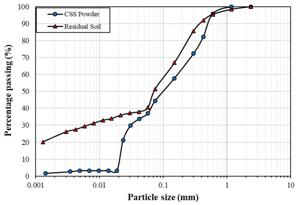
2.1.1. Tropical Residual Soil

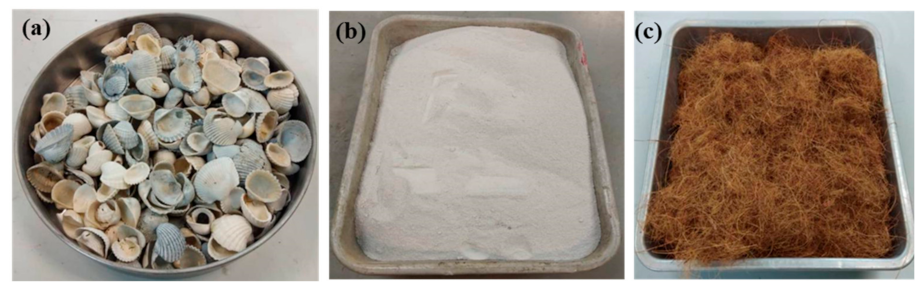
A typical Malaysian lateritic residual soil collected from a hillside located at Bandar Pinggiran Subang, Malaysia, was utilized in this study. Disturbed samples were manually collected from trial pits approximately 3 m below the ground’s surface using a shovel and a pickaxe. Bagged and labelled soil samples were then transported to the soil laboratory for testing. The basic engineering properties of the soil are listed in

Table 1. Basic engineering properties of the residual soil.

Property	Value
Sand (%)	48.56
Clay (%)	20.22
Gravel (%)	-
Silt (%)	31.22
D50 (mm)	0.07
Plastic limit (%)	21.80
Liquid limit (%)	50.10
Plasticity index (%)	28.30
Fines content	51.44
Activity	1.40
Linear shrinkage (%)	8.57
MDD (g/cm3) 1	1.82
OMC (%) 2	18.50
UCS (kPa) 3	153.11
FS (kPa) 4	125.15
ITS (kPa) 5	137.98
pH	9.31
Specific gravity	2.62

¹ MDD = maximum dry density; ² OMC = optimum moisture content; ³ UCS = unconfined compressive strength; ⁴ FS = flexural strength; ⁵ ITS = indirect tensile strength.

, while

Table 2. Significant oxides in the residual soil.

Significant Oxides	Concentration (wt.%)
SiO2	55.35
Al2O3	28.68
Fe2O3	5.93
TiO2	1.10
CaO	0.01
Na2O	0.03
K2O	0.32
MgO	0.16
P2O5	0.07
SO3	0.15
LOI	8.20

presents the significant oxides in the soil determined via X-ray fluorescence (XRF) analysis. Detailed discussion and test procedures on the XRF technique are outlined in [41]. Figure 1 shows the grain size distribution of the soil.

2.1.2. Seashells

The seashells (Figure 2a) used in this study were hand-picked from Pantai Remis beach, Selangor, Malaysia. The collected seashells were rinsed multiple times using deionized water to remove any interfering materials and were later oven-dried at 100 °C for 24 h. The cleaned–dried seashells were mechanically crushed to pass through a 2 mm sieve to obtain a homogeneous particle size distribution. The sieved samples were then subjected to calcination in a furnace. The heating process was performed at 900 °C for 120 min to activate quicklime from the calcite in the seashells. The physico-chemical properties of the CSS (see Figure 2b) are presented in

Table 3. Physico-chemical properties of the CSS.

Significant Oxides	Concentration (wt.%)
CaO	99.24
Fe2O3	0.16
SrO	0.40
Cr2O3	0.20
D50 (mm)	0.1
CC	0.25
CU	9.0
Sand (%)	55.52
Silt (%)	42.75
Clay (%)	1.73
Specific gravity	2.74

. The major oxides were also determined via XRF analysis. The grading curve of the CSS powder is shown in Figure 1.

2.1.3. Coir Fibre

The lightweight natural brown mature coir fibres (Figure 2c) used in the study were procured from a factory in Batu Pahat District, Johor, Malaysia. The coir fibres were cut to an average length of 12–25 mm. The physico-chemical properties of the coir fibres provided by the supplier are shown in

Table 4. Physico-chemical properties of the coir fibres.

Properties	Values
Chemical composition
Ash (%)	3
Cellulose (%)	41
Lignin (%)	46
Water soluble (%)	6
Chemical composition
Unit weight (g/cm3)	1.35
Breaking elongation (%)	28
Tensile strength (MPa)	65–140

.

2.2. Methods

2.2.1. Modification of Coir Fibre by Alkali Treatment

Based on a review of several studies [57,58,59,60,61,62], the following steps were employed for the alkali treatment of the coir fibres to impart hydrophobicity to the fibres, thereby increasing their life span, as well as to improve the interfacial bond strength. In order to remove the dust and debris, the fibres were washed twice with deionized water. The washed filaments were then dried at room temperature for two days. The dried coir fibres with known weights were soaked in 5% weight. After 24 h in a NaOH solution, the fibres were removed from the beaker and rinsed eight times with distilled water to remove any remaining alkali from the fibres’ surfaces. Next, the washed fibres were dried at room temperature for four days. The dried fibres were then preserved in airtight plastic containers to prevent contamination.

2.2.2. Soil Sample Preparation

To achieve a constant mass, the soil samples were oven-dried for three days at 105 °C. After that, the dried samples were manually crushed into smaller sizes. Before testing, the pulverized soil samples were mixed with the desired amounts of CSS and CF (see

Table 5. Experimental ranges and levels of the independent variables coded for the RCCD.

Independent Variable	Symbol	Values
	Chemical composition	−α −1.682	Low −1	Medium −1	High −1	+α +1.682
Calcined seashell content (wt.%)	A	0.61	3	6.5	10	12.39
Coir fibre content (wt.%)	B	0.005	0.08	0.19	0.3	0.38
Curing duration (days)	C	1	4	8	12	15

) by the mass of the dry soil. To facilitate the presentation of the results, a characterized sample designation scheme was used. For instance, 3% CSS + 0.08% CF represented 3% calcined seashell + 0.08% coir fibre-treated soil.

2.2.3. Testing Methods: Geotechnical Tests

The grain size distributions of the soil and the CSS powder were determined using both wet sieving and hydrometer analysis following the standard specification presented in [42]. The plasticity characteristics and particle density were determined using the standard specifications in [63,64]. The compaction characteristics of the untreated and treated soil samples were determined using the British Standard Light Compaction method. The tests were conducted following the standard procedures outlined in [64].

An unconfined compressive strength (UCS) test was conducted on the untreated and treated soil samples as per the standard specification in [64]. The UCS test was conducted by curing the samples in sealed vinyl bags for the specified time (see

Table 6. Experimental design matrix with three independent variables expressed in actual and coded units and experimental responses.

	Independent Variables in Coded Form			Independent Variables in Actual Form			Dependent Variables
Standard Run No.	A	B	C	A (%)	B (%)	C (Days)	UCS kPa	FS kPa	ITS kPa
1	−1	−1	−1	3	0.08	4	528.11	233.66	277.49
2	+1	−1	−1	10	0.08	4	771.19	249.78	392.88
3	−1	+1	−1	3	0.3	4	584.41	300.50	284.30
4	+1	+1	−1	10	0.3	4	876.37	327.83	442.45
5	−1	−1	+1	3	0.08	12	699.64	291.53	362.60
6	+1	−1	+1	10	0.08	12	944.03	306.76	518.57
7	−1	+1	+1	3	0.3	12	777.01	381.46	406.15
8	+1	+1	+1	10	0.3	12	969.42	502.40	536.26
9	−α	0	0	0.61	0.19	8	305.88	290.72	157.13
10	+α	0	0	12.39	0.19	8	1074.01	447.39	571.61
11	0	−α	0	6.5	0.005	8	837.46	278.88	418.06
12	0	+α	0	6.5	0.38	8	890.48	659.10	464.76
13	0	0	−α	6.5	0.19	1	411.92	287.85	188.80
14	0	0	+α	6.5	0.19	15	1043.11	582.10	547.34
15	0	0	0	6.5	0.19	8	912.29	536.50	507.52
16	0	0	0	6.5	0.19	8	912.37	536.62	507.63
17	0	0	0	6.5	0.19	8	912.25	536.45	507.47
18	0	0	0	6.5	0.19	8	912.32	536.55	507.56
19	0	0	0	6.5	0.19	8	912.30	536.53	507.60
20	0	0	0	6.5	0.19	8	912.20	536.40	507.43

) in a controlled room with a humidity of 98% and a temperature of ~20 ± 1 °C. An Instron automated loading machine was used to test cylindrical samples with a diameter of 50 mm and a length of 100 mm. The vertical load rate remained constant until the sample failed at 1 mm/min. For each combination, samples were prepared in triplicate, and the mean value was reported to guarantee the results‘ reliability. The variation in the UCS from the average strength should be less than ±8%, which was deemed acceptable and mirrored the effectiveness of the sample preparation method technique, as the singular strength did not deviate by more than ±10%, as suggested by [65].

A flexural strength (FS) test was conducted following the guidelines provided in [66]. The same procedures used for the UCS samples were used to prepare and cure the soil samples. The FS tests were carried out on an automated Instron machine at a monotonic load speed and support span of 1 mm/min and 140 mm, respectively, until the samples failed. Three duplicate samples of each combination were examined to guarantee the outcome’s consistency using Equation (1).

$$\mathrm{FS}=\frac{\mathrm{PL}}{{\mathsf{\pi }\mathrm{r}}^3}$$

(1)

where FS is the flexural strength, P is the maximum applied load, L is the span length, and r is the radius of the sample.

An indirect tensile strength (ITS) test was carried out by applying load along the cylindrical samples between two plates with reference to the indirect Brazilian test, as described by [67,68], using an automated Instron loading machine. The test was conducted on cylindrical samples with diameters and lengths of 50 mm and 100 mm, respectively. A loading rate of 1 mm/min was applied to the samples until failure. The ITS was determined by Equation (2). Triplicate samples of each combination were prepared and tested in order to guarantee the reliability of the result.

$$\mathrm{ITS}=\frac{2\mathrm{P}}{\mathsf{\pi }\mathrm{LD}}$$

(2)

where ITS is the indirect tensile strength, P is the maximum applied load, and L and D are the length and diameter of the sample, respectively.

2.2.4. Testing Methods: Microstructural Tests

To assess the mechanisms through which the soil was stabilized, as well as to observe the microstructural changes in the soil treated with both CSS and CF, X-ray diffraction (XRD) and Field Emission–Scanning Electron Microscopy (FESEM) tests were performed.

An XRD test was conducted on the untreated and treated samples using a Bruker D8-Focus diffractometer with a nickel-filtered Cu-Kα tube. X-rays with a wavelength of 1.5418 Å were adopted with a continuous mode Gonio scan between 2-theta positions of 5° and 91° with a scan step size of 0.03°. A current and voltage of 40 mA and 40 kV, respectively, were set in the generator.

FESEM analysis was performed using a dispersive X-ray spectrometer fixed with a Horiba X-Max detector. Both treated and untreated soil samples were mounted on aluminium sample holders with adhesive carbon tape and vacuum-coated with platinum for 40 s using a Quorum/Q150RS Sputter Coater (Monash University Malaysia NAP iLab, Bandar Sunway, Malaysia) before testing. The samples were then examined under a SU8010 FESEM operating at a current and voltage of 9400 nA and 5000 volts, respectively.

2.3. Response Surface Methodology (RSM)

RSM is a statistical technique aimed at developing regression models and optimizing various responses based on several independent variables through the analysis of quantitative data obtained from an experimental design [53,69,70]. Relative to other statistical techniques of experimental design, RSM assesses multiple parameters and their interactions by performing a reduced number of experimental trials. Optimization by RSM constitutes three major stages. First, statistically designed experiments are performed for the tolerable and dependable measurement of the response of interest. Next, a best-fit numerical model of the response surface is constructed. This is followed by determining the optimum experimental variables that yield a maximum or minimum response value, and, lastly, predicting the response through two- and three-dimensional plots and checking the model’s adequacy [49,54].

2.3.1. Experimental Design

In the current study, the experiments were designed by employing the rotatable central composite design (RCCD) with three independent variables (CSS content, CF content, and curing time) and five levels (±α, ±1, 0) (where α = 2^(3/4) = 1.682), as seen in Table 5. The response variables were UCS, FS, and ITS. Six replicates with standard run numbers ranging from 15 to 20 located at the centre of the design were employed to estimate the error sum of squares. The complete experimental design matrix developed utilizing the Design-Expert Version 11 software package, along with the responses, are summarised in Table 6.

In general, the total number of tests for a RCCD is 2n + 2n + nc, including the standard 2n factorial points with the origin at the centre, 2n points fixed axially at a distance, such as α (α = 2^(n/4)), from the centre to generate the quadratic terms, and the replicate runs at the centre (nc), where n is the number of independent variables. For the three independent variables considered in the current study, eight factorial points, six axial points, and six replicates at the central point were utilized for the RCCD. Thus, the total number of tests (N) required for the three independent variables is 20, as depicted in Equation (3) below [53].

$$\mathrm{N}=2^{\mathrm{n}}+2\mathrm{n}+{\mathrm{n}}_{\mathrm{c}}=2^3+\left(2\times 3\right)+6=20$$

(3)

2.3.2. Model Development and Optimization

RSM requires an empirical model to establish the relationship between the independent variables and the responses. A first-order linear model that fits the independent variables and responses, as given in Equation (4) [52], is often used.

$$\mathrm{Y}={\mathsf{\beta }}_0+{\mathsf{\beta }}_1{\mathrm{X}}_1+{\mathsf{\beta }}_2{\mathrm{X}}_2+\cdots +{\mathsf{\beta }}_{\mathrm{n}}{\mathrm{X}}_{\mathrm{n}}+\mathrm{e}$$

(4)

where ${\mathrm{X}}_1$, ${\mathrm{X}}_2$,… ${\mathrm{X}}_{\mathrm{n}}$ are the independent variables, ${\mathsf{\beta }}_0$ is the constant coefficient, ${\mathsf{\beta }}_1$, ${\mathsf{\beta }}_2$,… ${\mathsf{\beta }}_{\mathrm{n}}$ are the unknown regression coefficients, and e is the error observed in the response Y.

However, if the developed first-order linear model insufficiently estimates the curvature at the response surface, then a second-order or higher-level polynomial model containing quadratic terms must be used, as shown in Equation (5) [71].

$$\mathrm{Y}={\mathsf{\beta }}_{\mathrm{O}}+{\displaystyle \sum }_{\mathrm{i}=1}^{\mathrm{n}}{\mathsf{\beta }}_{\mathrm{i}}{\mathrm{X}}_{\mathrm{i}}+{\displaystyle \sum }_{\mathrm{i}=1}^{\mathrm{n}}{\mathsf{\beta }}_{\mathrm{ii}}{\mathrm{X}}_{\mathrm{i}}^2+{\displaystyle \sum }_{\mathrm{i}=1}^{\mathrm{n}}{\displaystyle \sum }_{\mathrm{j}=1}^{\mathrm{n}}{\mathsf{\beta }}_{\mathrm{ij}}{\mathrm{X}}_{\mathrm{i}}{\mathrm{X}}_{\mathrm{j}}+\mathrm{e}$$

(5)

where Y is the anticipated response, n is the total number of factors investigated, i and j are the index numbers of the factors, ${\mathsf{\beta }}_{\mathrm{O}}$ is the offset term known as the intercept term, ${\mathsf{\beta }}_{\mathrm{ij}}$ (i = 1, 2,…, n; j = 1, 2,…, n) are the interaction coefficients, ${\mathsf{\beta }}_{\mathrm{i}}$ (i = 1, 2,…, n) are the linear coefficients, ${\mathsf{\beta }}_{\mathrm{ii}}$ (i = 1, 2,…, n) are the quadratic coefficients, ${\mathrm{X}}_{\mathrm{i}}$ and ${\mathrm{X}}_{\mathrm{j}}$ are the coded independent variables, and e is the residual error between the predicted and the real experimental values. The second-order quadratic model was used for this study as an excellent model to evaluate the real response surface.

The optimization of the multiple responses was carried out using the desirability function (D) [72], as shown in Equation (6).

$$D={\left(d_1\times d_2\times \dots d_m\right)}^{1/m}={\left({{\displaystyle \prod }}_{i=1}^m{d}_i\right)}^{1/m}$$

(6)

where m represents the total number of responses used in the optimization research and d_i represents the response’s desirability. D is a function that measures how desirable (well-matched) the dependent variables are with the independent variables at a particular level. D can have a value between 0 and 1. All the variables that are being simultaneously optimised can be thought of as having a desired value if D reaches a value that is not zero. On the other hand, D will be zero if one or more responses are outside of the desired bounds, d_i = 0.

2.3.3. Statistical Analysis

Design-Expert software was utilized for the determination of the regression coefficients of the quadratic models for the experimental data and for evaluating the model’s adequacy and statistical significance. Analysis of variance (ANOVA) was employed to define the interaction between the independent variables and the responses. The statistical significance was determined by the F-test using the same program. To evaluate different interactions of any two independent variables while keeping the value of the third variable fixed at the central (0) level, response surface and contour plots were developed.

3. Results and Discussion

3.1. Effect of CSS Powder and Treated CF on Geotechnical Properties

3.1.1. Atterberg Limits

Table 7. Experimental range and levels of the independent variables coded for the RCCD.

Soil Mixture	LL (%)	PL (%)	PI (%)	Soil Mixture	LL (%)	PL (%)
0% CSS + 0% CF (control)	50.10	21.80	28.30	0% CSS + 0% CF (control)	50.10	21.80
3% CSS + 0.08% CF	39.80	16.84	22.96	3% CSS + 0.08% CF	39.80	16.84
10% CSS + 0.08% CF	36.0	15.04	20.96	10% CSS + 0.08% CF	36.0	15.04
3% CSS + 0.3% CF	35.20	15.31	19.89	3% CSS + 0.3% CF	35.20	15.31
10% CSS + 0.3% CF	30.40	13.31	17.09	10% CSS + 0.3% CF	30.40	13.31
0.61% CSS + 0.19% CF	45.71	19.01	26.70	0.61% CSS + 0.19% CF	45.71	19.01
12.39% CSS + 0.19% CF	30.70	16.37	14.33	12.39% CSS + 0.19% CF	30.70	16.37
6.5% CSS + 0.005% CF	35.30	16.22	19.08	6.5% CSS + 0.005% CF	35.30	16.22
6.5% CSS + 0.19% CF	35.70	17.66	18.04	6.5% CSS + 0.19% CF	35.70	17.66
6.5% CSS + 0.37% CF	35.60	17.72	17.88	6.5% CSS + 0.37% CF	35.60	17.72

presents the results of the Atterberg limits of the stabilized soil under different additive contents. As observed from Table 7, the liquid limit (LL) decreased with increasing CSS and CF contents from 0% to 12.38% and 0% to 0.37%, respectively. The maximum reduction in the LL (30.40%) was obtained with the addition of 10% CSS and 0.3% CF. The plastic limit (PL) and plasticity index (PI) of the soil presented a similar variation tendency upon the addition of CSS and CF. The PL decreased from 21.80% to 13.31% upon the addition of 10% CSS and 0.3% CF. An analogous reduction in the PI from 28.30% to 14.33% was noted upon the addition of 12.39% CSS and 0.19% CF. The percentage reductions in the LL, PL, and PI of the stabilized soil were about 39%, 39%, and 49%, respectively, over the untreated soil.

The chemical reaction (ion exchange) between the CSS-CF and soil decreased the plasticity characteristics of the treated soil samples. The electrolyte concentration of the pore fluid increased when Ca²⁺ ions from the CSS dissolved into it, causing a decrease in the thickness of the soil’s diffuse double layer (DDL). A thinner DDL makes the soil less active and plastic, lowering the LL. Additionally, this behaviour may be brought on by CSS powder dissociation into Ca²⁺ and OH after water dissolution. The clay particles in the treated soil may undergo an ion exchange (such as Na⁺) for Ca²⁺ as a result of this dissociation. Consequently, the ion exchange could promote mineral particle agglomeration and PI reduction [73,74]. Alkali treatment can also reduce the water absorption capacity of fibres, which can result in lower plasticity characteristics for the treated soil. A decreasing PI in CSS powder-CF treated soil samples indicates an increase in workability, as it limits the range of moisture content, where soil is susceptible to compaction. Moreover, a lower PI indicates a lower shrink–swell behaviour for treated soil [75].

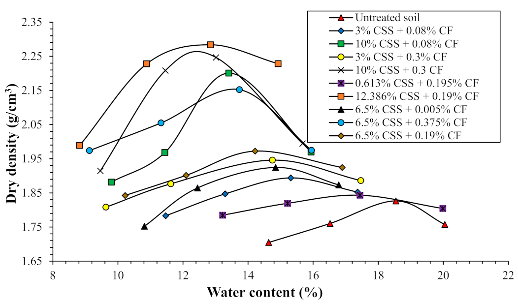
3.1.2. Compaction Characteristics

Figure 3 presents the compaction characteristics of the untreated and treated soil samples. Evidently, increasing the CSS and CF contents led to an increase in the MDD and a decrease in the OMC. When the CSS and CF contents increased from 0% to 12.39% and 0% to 0.19%, respectively, the MDD reached the highest value of 2.28 g/cm³ with a corresponding OMC of 12.8%. In contrast, the MDD reached the lowest value of 1.82 g/cm³ with a corresponding OMC of 18.5% for the untreated soil. The decrease in OMC may have been a result of two main factors: the low water affinity of CSS powder relative to the soil, and the decrease in the number of voids in the soil–fibre matrix. The decrease in the plasticity characteristics of the treated soil supports the first factor. In addition to the reduction in the number of voids, the low water absorption capacity of the fibre due to the alkali treatment would have also reduced the OMC [76].

Both the particle density and grain size of the CSS powder and soil might have increased the MDD. In particular, the MDD may have been increased by the high particle density of the CSS powder (2.74) compared with the soil (2.62), which thus increased the average unit weight of the compacted soil solids in the mixture. A better interaction of the CF with the soil decreased the pore size between the soil matrix by filling the gaps between the soil particles [77]. This enhanced the MDD of the treated soil and strengthened the bonding between soil particles. As increasing the MDD indicated improvements in the soil strength (e.g., [78,79]) the treated soil had the potential to be utilized as a construction material.

3.1.3. Unconfined Compressive Strength

Table 6 presents the results of the UCS tests conducted on various combinations of soil–CSS–CF mixtures for different curing periods. It is evident that the addition of CSS powder and CF resulted in an increase in the soil’s UCS when the results of the UCS test are compared with those of the untreated soil (153.11 kPa) for various curing periods.

There are four main reasons why the UCS of the treated soil could have increased its strength: (1) Cation exchange between the monovalent ions (such as Na⁺) on the surface of the soil particles and the Ca²⁺ ions in the CSS powder. The soil particles may agglomerate and flocculate as a result of this process, becoming more rigid, brittle, and coarse, which may increase the soil matrix’s ability to resist friction [76]. This confirms the marginal improvement in the UCS at the early stage of curing. (2) Pozzolanic reactions that warrant long-term strength development. The soil’s silica or alumina and Ca²⁺ in the CSS powder may undergo a time-dependent reaction known as the pozzolanic reaction, which would result in the development of cementitious calcium aluminate hydrate (C-A-H) and calcium silicate hydrate (C-S-H) phases that bind the soil’s particles together (Equations (7)–(10)).

$$\mathrm{CaO}+{\mathrm{H}}_2\mathrm{O}\to \mathrm{Ca}{\left(\mathrm{OH}\right)}_2$$

(7)

$$\mathrm{Ca}{\left(\mathrm{OH}\right)}_{2 }\to {\mathrm{Ca}}^{2+}+2\left({\mathrm{OH}}^{-}\right)$$

(8)

$${ \mathrm{Ca}}^{2+}+2\left({\mathrm{OH}}^{-}\right)+{\mathrm{SiO}}_2\left(\mathrm{soluble} \mathrm{clay} \mathrm{silica}\right)\to \mathrm{Calcium} \mathrm{silicate} \mathrm{hydrate}$$

(9)

$${\mathrm{Ca}}^{2+}+2\left({\mathrm{OH}}^{-}\right)+{\mathrm{Al}}_2{\mathrm{O}}_3\left(\mathrm{soluble} \mathrm{clay} \mathrm{alumina}\right)\to \mathrm{Calcium} \mathrm{aluminate} \mathrm{hydrate}$$

(10)

(3) The enhancement in the UCS may also have been a result of the interlocking force created by a spatial network of distributed CF in the cemented soil matrix. This interlocking force would increase the friction between the fibres and soil matrix, increase the bonding strength, and prevent the movement of the fibre–soil matrix [80,81,82]. (4) The improvement in the UCS could also be explained by the excellent adhesion between the soil matrix and the CF [83].

3.1.4. Flexural Strength

The results of the FS for the soil samples treated with CSS powder and CF for a variety of curing periods are shown in Table 6. The UCS results are in line with the results of the FS test. It is evident that the addition of CSS powder and CF increased the soil’s FS when comparing the FS values of the treated and untreated samples (125.15 kPa). The fibre’s soil-interlocking ability would improve the FS. Consequently, this would restrict the relative displacement of the particles and increase the bond strength and friction between the fibres and soil [82,84,85,86]. Additionally, the inclusion of the treated fibre in the soil would lead to adequate bonds in the CSS powder-treated soil’s interaction zone, resulting in an increment in FS [30]. When the samples were loaded, loads could be transferred through shear.

3.1.5. Indirect Tensile Strength

The ITS results of the treated soil samples for various curing periods compared with the untreated soil (137.98 kPa) show that, with the addition of CSS powder and CF, the ITS of the soil was improved (Table 6). The pozzolanic reaction between the CSS powder and the soil formed C-A-H and C-S-H phases in the soil, increasing the ITS of the treated soil. These cementitious compounds are characterized by high strength. Additionally, the rough surface area of the treated soil, as observed in Figure 14e, supported the effective contact area between the fibre and the soil. This increased the interfacial friction between the two materials, possibly improving the ITS [57,78]. Li et al. [85] linked the increment in the ITS to increasing dry density. They postulated that a high dry density enhanced the contact between soil particles by improving the bonding force of soil particles. Additionally, the increased dry density also increased the fibre/soil interfacial contact area, which enhanced the interfacial shear strength. Collectively, these characteristics yielded a higher tensile strength.

Li et al. [87] further showed that decreasing water content increased the ITS through the following two aspects: (1) Cohesion and suction increase with decreasing water content, thus strengthening the bonds between soil particles. (2) The decrease in water content could strengthen the interfacial mechanical interactions between the fibre and soil matrix and increase the capability of the fibre to bear the tensile load. Hence, the corresponding increase and decrease in the MDD and OMC, respectively, were key factors in improving the ITS of the treated soil. Moreover, the CSS powder and treated CF significantly improved the mechanical characteristics of the soil in terms of its UCS, ITS, and FS.

3.2. Regression Model and Statistical Assessment

3.2.1. Regression Model Development

The reduced quadratic model was thought to be the best fit for independent variables and responses when multiple regression analysis is applied to a design matrix and responses. Equations (11)–(13) present the coded factor-based final regression models for the UCS, FS, and ITS, respectively.

$$\mathrm{UCS}=810.06+165.75\mathrm{A}+25.88\mathrm{B}+123.86\mathrm{C}-12.28\mathrm{AC}-1.06{\mathrm{B}}^2$$

(11)

$$\mathrm{FS}=539.52+32.45\mathrm{A}+78.34\mathrm{B}+63.36\mathrm{C}+11.59\mathrm{AC}-78.89{\mathrm{A}}^2-43.56{\mathrm{B}}^2-55.59{\mathrm{C}}^2$$

(12)

$$\mathrm{ITS}=438.31+92.02\mathrm{A}+14.36\mathrm{B}+75.38\mathrm{C}+1.57\mathrm{AC}-11.18{\mathrm{B}}^2$$

(13)

where the independent variables of the CSS content, CF content, and curing time are represented by the coded terms A, B, and C, respectively. Equations (14)–(16) present the final regression models for the UCS, FS, and ITS in terms of actual factors, respectively.

$$\begin{array}{c}\mathrm{UCS}=161.05041+54.37537\times \mathrm{CSS} \mathrm{content}+268.40757\times \mathrm{CF} \mathrm{content}+\\ 36.66666\times \mathrm{curing} \mathrm{time}-0.877143\times \mathrm{CSS} \mathrm{content}\times \mathrm{curing} \mathrm{time}-\\ 87.25080\times {\mathrm{CF} \mathrm{content}}^2\end{array}$$

(14)

$$\begin{array}{cc}\hfill \mathrm{FS}=-364.11058& +86.36880\times \mathrm{CSS} \mathrm{content}+2080.17273\times \mathrm{CF} \mathrm{content}\hfill \\ & +66.04312\times \mathrm{curring} \mathrm{time}\hfill \\ & +0.827857\times \mathrm{CSS} \mathrm{content}\times \mathrm{curing} \mathrm{time}\hfill \\ & -6.44011{ \mathrm{CSS} \mathrm{content}}^2-3599.91774{ \mathrm{CF} \mathrm{conetnt}}^2\hfill \\ & -3.47407\times {\mathrm{curing} \mathrm{time}}^2\hfill \end{array}$$

(15)

$$\begin{array}{cc}\hfill \mathrm{ITS}=64.32212& +25.39542\times \mathrm{CSS} \mathrm{content}+481.65803\times \mathrm{CF} \mathrm{content}\hfill \\ & +18.11716\times \mathrm{curing} \mathrm{time}\hfill \\ & +0.111964\times \mathrm{CSS} \mathrm{content}\times \mathrm{curing} \mathrm{time}\hfill \\ & -923.89760\times {\mathrm{CF} \mathrm{content}}^2\hfill \end{array}$$

(16)

In terms of coded and actual factors, the aforementioned models are useful for determining the relative impact of the factors by comparing the factor coefficients, as well as for predicting the responses at specific levels of each factor.

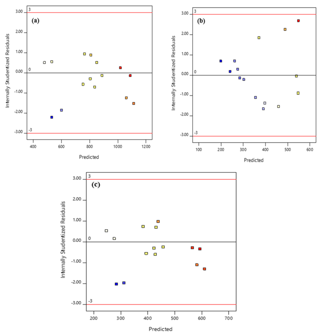
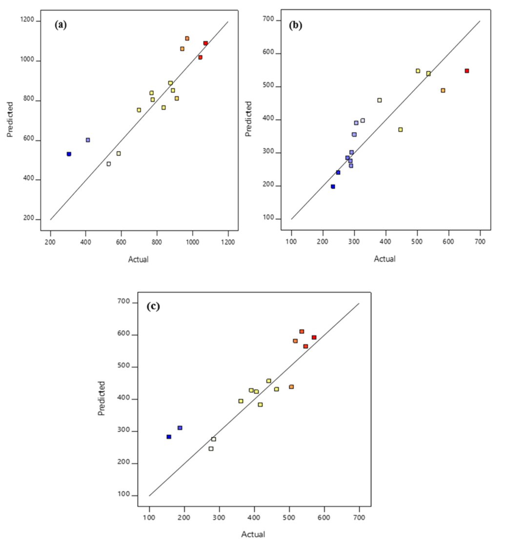
3.2.2. Statistical Assessment of Experimental Results

The simplified quadratic model was determined to be the model with the best fit for the independent variables and responses by conducting multiple regression analyses on the design matrix and the responses. Equations (11)–(13) present the final regression models for the UCS, FS, and ITS in terms of coded factors, respectively.

Statistical analysis for the response surface reduced quadratic model for UCS.

The corresponding coefficient becomes more significant at larger F-values (smaller p-values) [48]. The model had an F-value of 8.15 and a very low p-value (0.0009), indicating that it was significant (

Table 8. ANOVA for response surface reduced quadratic model for UCS.

Source	Sum of Squares	DF	Mean Square	F-Value	p-Value	Remarks
Model	5.951 × 105	5	1.190 × 105	8.15	0.0009	Significant
A—CSS content	3.752 × 105	1	3.752 × 105	25.69	0.0002	Significant
B—CF content	9145.42	1	9145.42	0.6262	0.4419
C—Curing time	2.095 × 105	1	2.095 × 105	14.35	0.0020	Significant
AC	1206.39	1	1206.39	0.0826	0.778
B2	16.36	1	16.36	0.0011	0.9738
Residual	2.045 × 105	14	14,604.32
Lack of fit	2.045 × 105	9	22,717.82
Pure error	0.0000	5	0.0000
Correlation total	7.996 × 105	19	R2	0.7443
Mean	809.34		Adjusted R2	0.6530
C.V. (%)	14.93		Predicted R2	0.4780 response surface reduced quadratic model
PRESS	4.173 × 105		Adequate precision	9.5327

DF = Degrees of freedom; PRESS = Predicted residual sum of squares; C.V. = Coefficient of variation.

). There was only a 0.09% probability that this large of an F-value would be seen due to noise. Only when the p-values are less than 0.05 do the model terms become significant. The major model terms in this instance were the main effects of the CSS content (A) and curing time (C). The p-values greater than 0.05 for other model terms denoted a lower level of significance. The percentage contribution of each term to the UCS is displayed in Figure 4a.

A comparison of the range of predicted values at the design space indicates the average prediction error, which is an adequate precision measure of the signal-to-noise ratio. The ideal ratio is greater than 4. The ratio of 9.5327 in this situation denotes a strong signal. The model can, therefore, be used to explore the design space. The determination coefficient (R²) shows how accurate a model is. According to the computed R² value for the UCS (0.7443), the independent variables were responsible for 74.43% of the sample variation in the UCS, leaving the model to account for just roughly 25.57% of the overall variation. This shows that the regression model had good overall capability and precision. With a difference of less than 0.2 and a decent agreement between the anticipated R² of 0.4780 and the adjusted R² of 0.6530, there was a strong correlation between the observed and predicted values. These findings imply that the regression model explained the relationship between the independent variables and the response quite well (UCS).

Statistical analysis of the response surface reduced quadratic model for FS.

Table 9. ANOVA for the response surface reduced quadratic model for FS.

Source	Sum of Squares	DF	Mean Square	F-Value	p-Value	Remarks
Model	2.915 × 105	7	41,635.93	9.56	0.0004	Significant
A—CSS content	14,376.91	1	14,376.91	3.30	0.0943
B—CF content	83,819.46	1	83,819.46	19.24	0.0009	Significant
C—Curing time	54,818.87	1	54,818.87	12.58	0.004	Significant
AC	1074.62	1	1074.62	0.2467	0.6284
A2	89,693.67	1	89,693.67	20.59	0.0007	Significant
B2	27,343.79	1	27,343.79	6.28	0.0276	Significant
C2	44,526.65	1	44,526.65	10.22	0.0077	Significant
Residual	52,272.80	12	4356.07
Lack of fit	52,272.77	7	7467.54	1.249 × 106	<0.0001	significant
Pure error	0.0299	5	0.0060
Correlation total	3.437 × 105	19	R2	0.8479
Mean	417.95		Adjusted R2	0.7592
C.V. (%)	15.79		Predicted R2	0.2635
PRESS	2.532 × 105		Adequate precision	8.3642

presents the results of the reduced quadratic model in the form of an ANOVA test for the FS. As shown in the table, the model had an F-value of 9.56 and a p-value of 0.0004, indicating that the model was significant. Hence, there was only a 0.04% probability that such a large F-value could occur due to noise. The main effects of the CF content (B) and curing time (C), as well as the quadratic effects of the CSS content (A2), CF content (B2), and curing time (C2) were found to be the significant model terms. Other model terms with p-values of >0.05 were considered insignificant. Based on the obtained F-values, the ranking of the significant model terms was as follows: A2 > B > C > C2 > B2. Figure 4b shows the percentage contribution of each model term to the FS. The lack of fit F-value of 1,249,448.63 indicates that the lack of fit was significant. Hence, there was only a 0.01% probability that such a large lack of fit F-value could occur due to noise. The R² value of 0.8479 demonstrated that the sample variation of 84.79% was due to the independent variables, and only about 15.21% of the entire variation could not be elucidated by the model. The predicted R² of 0.2635 was not as close to the adjusted R² of 0.7592 as one might normally expect, i.e., the difference was >0.2. This may have been due to a large block effect or outliers. Nonetheless, an adequate precision of 8.3642 was recorded, which was well above 4, thus indicating an adequate signal. Hence, the developed model could be employed to navigate the design space.

Statistical analysis for the response surface reduced quadratic model for ITS.

Similar results of the simplified quadratic model for the ITS are shown in

Table 10. ANOVA for the response surface reduced quadratic model for ITS.

Source	Sum of Squares	DF	Mean Square	F-Value	p-Value	Remark
Model	1.979 × 105	5	39,582.01	7.27	0.0015	Significant
A—CSS content	1.156 × 105	1	1.156 × 105	21.24	0.0004	Significant
B—CF content	2817.53	1	2817.53	0.5175	0.4838
C—Curing time	77,599.66	1	77,599.66	14.25	0.002	Significant
AC	19.66	1	19.66	0.0036	0.9529
B2	1833.93	1	1833.93	0.3368	0.5709
Residual	76,227.25	14	5444.80
Lack of fit	76,227.22	9	8469.69	1.443 × 105	<0.0001	Significant
Pure error	0.0294	5	0.0059
Correlation total	2.741 × 105	19	R2	0.7219
Mean	430.68		Adjusted R2	0.6226
C.V. (%)	17.13		Predicted R2	0.4634
PRESS	1.471 × 105		Adequate precision	8.9946

as an ANOVA. The model was implied to be significant by the model’s F-value of 7.27 and the associated p-value of 0.0015. The likelihood that noise would cause an F-value this high was 0.15% at most. The model terms are considered significant when the p-value is less than 0.05. The major model terms in this instance were the main effects of the CSS content (A) and cure time (C). The p-values greater than 0.05 for the other model terms indicate that the model terms were not significant. The percentage contribution of each term to the ITS is shown in Figure 4c. The lack of fit F-value of 1,442,877.62 implied that the lack of fit was significant. Noise was only 0.01% likely to have caused a lack of fit F-value of this magnitude. The ITS sample variation of 72.19% could be attributed to the independent variables and only about 27.81% of the total variation could not be explained by the model, as indicated by the R² value of 0.7219. The adjusted R² of 0.6226 and the predicted R² of 0.4634 were in reasonable agreement; i.e., the difference was less than 0.2, indicating that the observed and predicted values were highly correlated. This suggests that the relationship between the response and the independent variables was well explained by the regression model (ITS). The signal-to-noise ratio was measured with sufficient precision. The ideal ratio is greater than 4. For this situation, the proportion of 8.9946 was satisfactory. As a result, the model could be used to move around the design space.

In order to evaluate the model fitness, the residual plots were investigated, as shown in Figure 5, Figure 6 and Figure 7. The data distribution pattern was identified using the normal % probability versus the studentized residual plot. As shown in Figure 5, the internally studentized residuals were roughly plotted along the diagonal line, indicating that the model response had a normal distribution. Thus, the models accurately explained the relationship between the responses and the independent variables. Moreover, it also indicated that the errors were distributed normally; hence, the normality assumption was satisfied and no response transformation was needed. Figure 6 shows the random distribution of the residuals between ±3.0. There was no evidence to support any possible violations of the independence or constant variance assumptions, indicating that the fitted models’ approximations of the answers were generally valid [52]. The random distribution of the residuals also suggested that the variance of the original observations was constant for all values of the response, so the transformation of the response variable was not required [86]. Hence, the constant variance assumption of the least-squares was satisfied. Figure 7 demonstrates that the predicted response values are in good agreement with the actual ones in the range of the operating variables, as most of the values lie along the diagonal line. It is obvious from the pattern seen in Figure 5, Figure 6 and Figure 7 that the generated models are capable of accurately forecasting the experimental data.

3.3. Effects of the Independent Variables on the UCS, FS, and ITS

Three-dimensional (3D) response surface plots as a function of two variables, maintaining all other variables at constant levels, are vital in understanding the main effect, the quadratic effect, and the interactive effects of these two variables. Moreover, 3D response surfaces and their corresponding contour plots can facilitate the examination of the effects of the independent variables on the responses [83]. In this study, the RCCD and RSM were employed with three independent variables to assess their effects on the UCS, FS, and ITS. To investigate the interactive effects of two independent variables on the response values, three-dimensional surface and contour plots were developed by considering two variables at a time while keeping the other one constant at the central (0) level.

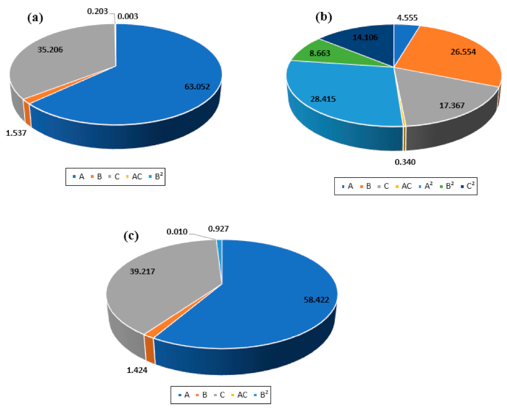
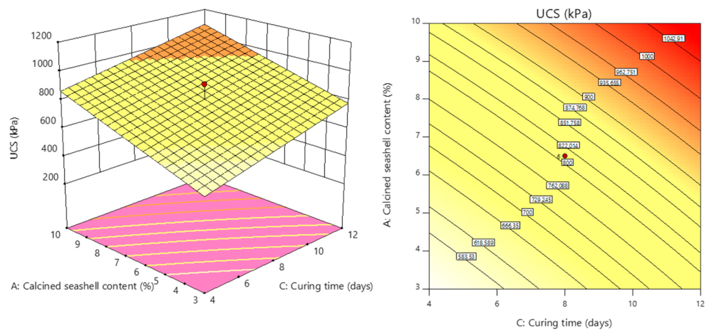
3.3.1. The Effect of Independent Variables on the UCS

In the previous section, the reduced quadratic model was developed for the effects of the three independent variables on the UCS. As there was only one interaction term in the model, the interactive effects of the CSS content (A) and curing time (C) on the UCS were studied by keeping the CF content (B) at the central level (0.19), and the result in the form of a 3D plot and its corresponding contour plot is presented in Figure 8. When the CSS content increased from 3% to 10% and the curing time increased from 4 to 12 days, the UCS increased almost linearly. Section 3.1.3 discusses the factors that led to an increase in the UCS when CSS powder was added and the curing time was extended. The findings, which were supported by the ANOVA analysis’s strong F-values, showed that, under the experimental conditions investigated, the amount of CSS and curing period had a substantial impact on the soil’s UCS in relation to the CF content. The maximum UCS of 1112.22 kPa was obtained when the CSS content was 10% and the curing time was 12 days.

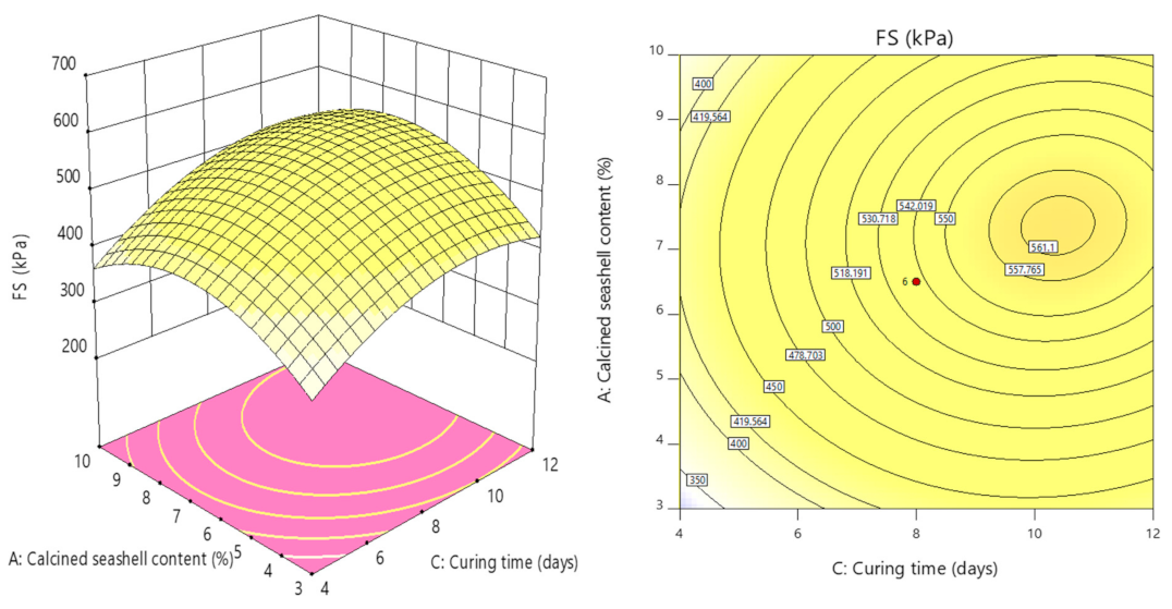
3.3.2. The Effect of Independent Variables on the FS

Similarly, Figure 9 shows a 3D surface plot and its related contour plot demonstrating how the FS is affected by the CSS content (A) and curing time (C) while maintaining the central level of the CF content (B) (0.19). As the CSS content and curing increased grew from 3% to roughly 6.5% and from 4 days to 8 days, respectively, it was found that the FS increased. The FS decreased with a further increase in the CSS content and curing time. The CSS content and curing time had a significant effect on the soil’s FS. In Section 3.1.4, it is explained why the FS increased with the addition of CSS powder and as the curing time increased. The maximum FS of 548.07 kPa was observed when the CSS content was 6.5% and the curing time was 8 days.

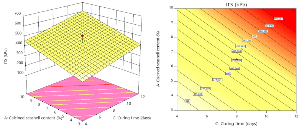
3.3.3. The Effect of Independent Variables on the ITS

Figure 10 shows the effects of the CSS content (A) and curing time (C) on the ITS while maintaining the CF content (B) at the central level (0.19). The effects of the CSS content and curing time on the ITS are similar to their effects on the UCS (Figure 8). The ITS increased consistently with increasing CSS content (3% to 10%) and curing time (4 to 12 days). Section 3.1.5 discusses the reasons why the addition of CSS powder and an increased curing period led to an increase in the ITS. The findings suggest that, under the experimental conditions investigated, the CSS content and the curing time had a significant impact on the soil’s ITS in relation to the CF content. This was supported by the ANOVA analysis’s high F-values. The maximum ITS of 610.46 kPa was obtained when the CSS content was 10% and the curing time was 12 days.

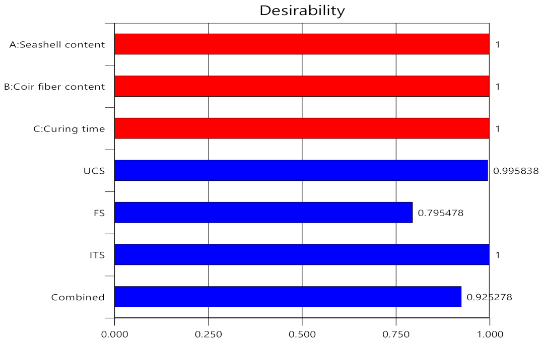
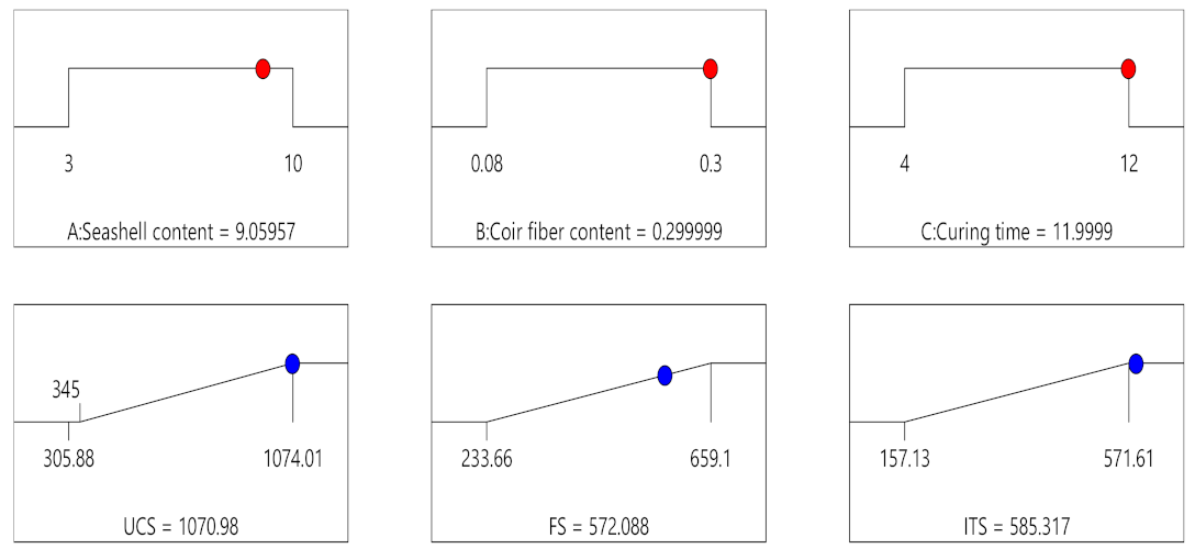
3.4. Optimization Analysis

The results of the optimization analysis are explained and discussed in detail in this section. The criteria for the optimization of all studied factors in correspondence with the responses are shown in

Table 11. Optimization of the individual responses (di) in order to obtain the overall desirability response (D).

Name	Goal	Lower Limit	Upper Limit	Lower Weight	Upper Weight	Importance
A: Seashell content	Is in range	3	10	1	1	3
B: Coir fibre content	Is in range	0.08	0.30	1	1	3
C: Curing time	Is in range	4	12	1	1	3
UCS	Maximize	345	1074.01	1	1	3
FS	Maximize	233.66	659.10	1	1	3
ITS	Maximize	157.13	571.61	1	1	3

. All independent variables’ lower and upper limit values were derived from the RCCD levels (see Table 5). The lower and upper limits of the FS and ITS responses were derived from the experimental data, whereas the lower limit for the UCS was established at 345 kPa in accordance with [84]. Figure 11 illustrates the individual desirability functions (di) for each response and the estimated geometric mean as the highest overall desirability (D = 0.925) for the first solution (see

Table 12. Optimized additive ratios and corresponding responses.

Solution Number	CSS Content	CF Content	Curing Time	UCS	FS	ITS	Desirability
1	9.06	0.30	12	1070.99	572.09	585.32	0.925
2	9.09	0.30	12	1072.15	571.54	586.04	0.925
3	9.04	0.30	12	1069.93	572.57	584.68	0.925
4	9.12	0.30	12	1073.59	570.85	586.92	0.925
5	9.01	0.30	12	1068.63	573.16	583.90	0.925
6	8.97	0.30	12	1067.12	573.83	582.97	0.925
7	9.10	0.29	12	1072.38	571.35	586.69	0.925
8	8.98	0.29	12	1067.03	573.82	583.36	0.925
9	9.07	0.30	12	1069.10	572.68	584.05	0.925
10	8.87	0.29	12	1062.30	575.85	580.33	0.925
11	8.93	0.30	12	1062.79	575.46	580.20	0.925
12	9.01	0.30	12	1065.27	574.26	581.65	0.925
13	8.71	0.29	12	1054.84	578.66	576.32	0.924
14	9.28	0.30	12	1074.01	569.29	586.75	0.924
15	9.08	0.28	12	1067.58	571.96	586.82	0.924
16	8.86	0.30	11	1049.57	579.62	571.61	0.923
17	9.32	0.24	12	1068.93	557.61	593.33	0.911
18	9.40	0.20	12	1063.75	536.62	592.63	0.889
19	6.63	0.28	12	962.33	584.09	521.12	0.849

). The desirability function for the independent variables (CSS, CF, and curing time) was equal to 1 because they were set to be in range in the optimization. The obtained desirability functions for UCS, FS, and ITS were 0.9958, 0.7955, and 1, respectively.

By employing this desirability function and setting a pre-selected goal for each factor, the optimized specific value for all responses to solution number 1 (see Table 12) was determined, and the results are shown in Figure 12. The optimal levels of the independent variables for achieving maximum UCS, FS, and ITS of 1070.98 kPa, 572.09 kPa, and 585.32 kPa, respectively, were a CSS content of 9.06%, a CF content of 0.30%, and a curing time of 12 days. In addition, Table 12 recommends 19 ideal options for achieving appropriate UCS, FS, and ITS values. Experimental runs employing the ideal conditions of solutions 1 to 10 in duplicate were used to validate the models.

Table 13. Validation of optimized model responses by experimental runs indicating the percentage errors.

Solution Number	Optimized Model Values			Experimental Run Values			Percentage Error
	UCS	FS	ITS	UCS	FS	ITS	UCS	ITS	FS
	kPa	kPa	kPa	kPa	kPa	kPa	(%)	(%)	(%)
1	1070.98	572.09	585.32	1054.21	564.05	573.96	1.59	1.43	2.44
2	1072.15	571.54	586.04	1058.41	560.22	572.06	1.30	2.02	2.44
3	1069.93	572.57	584.68	1048.32	565.38	569.77	2.06	1.27	2.62
4	1073.59	570.85	586.92	1055.09	558.79	571.05	1.75	2.16	2.78
5	1068.63	573.16	583.90	1050.02	564.98	570.43	1.77	1.45	2.36
6	1067.12	573.83	582.97	1043.56	562.11	567.32	2.26	2.09	2.76
7	1072.38	571.35	586.69	1058.02	559.32	573.85	1.36	2.15	2.24
8	1067.03	573.82	583.36	1041.78	562.78	568.64	2.42	1.96	2.59
9	1069.10	572.68	584.05	1044.21	560.34	570.77	2.38	2.20	2.33
10	1062.30	575.85	580.33	1040.98	566.21	563.99	2.05	1.70	2.90

displays the average values of the UCS, FS, and ITS, as well as the percentage inaccuracy in comparison with the model values. According to the findings, the experimental value and the optimal values predicted by the generated models agreed fairly well. The UCS, FS, and ITS for the CSS powder–CF-stabilized soil could, therefore, be predicted fairly accurately using the developed models.

3.5. Microstructural Properties

3.5.1. X-ray Diffraction

Figure 13a,b, and c show the XRD diffractograms of the CSS powder, untreated soil, and 9.06% CSS + 0.30% CF-treated soil after 12 days of curing, respectively. The analyses revealed that the dominant phases present in the CSS powder were CaO, calcite, and scheelite. The presence of CaO in the diffractogram agreed with the XRF analysis, and also confirmed the possibility of the pozzolanic reaction to occur.

The analyses also showed that goethite and quartz were the two main minerals found in both the treated and untreated soil samples. The minor phases that were observed were kaolinite and illite (Figure 13b,c). Previous reserachers [88,89] and Latifi et al. [74] reported similar mineral compositions for tropical residual soils. The existence of goethite and quartz was confirmed by the main reflections at 2θ of 21.56° (d = 4.12 Å) and 26.78° (d = 3.33 Å), respectively, for the untreated and treated soil samples. The intensity of the quartz reflection (2θ of 26.78°) appeared to be slightly lower for the treated soil, even though the diffractograms of the treated and untreated soil showed no significant differences. The impact of the CSS powder on the soil matrix may have been one cause of this decline. Owing to the stabilization process, the goethite reflection intensity (2θ = 21.56°) remained essentially unaffected. The presence of quartz in both diffractograms supported the XRF analysis’ conclusion that there was SiO₂ in the soil.

At different 2θ angles of 29.56°, 36.11°, and 47.68°, the treated soil appeared to have a number of additional reflections, as shown in Figure 13c. These reflections were linked to the development of C-S-H and C-A-H cementing phases, which filled soil pores and bound soil particles together to improve the treated soil’s mechanical performance. These reflections were absences in the untreated soil, which demonstrated that stabilization occurred due to pozzolanic process reactions.

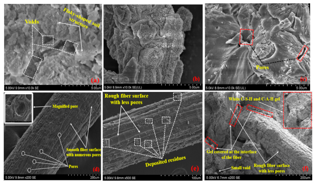
3.5.2. FESEM Analysis

The FESEM micrograph of the untreated soil is shown in Figure 14a. Due to the lack of pozzolanic products, the micrograph showed a discontinuous and somewhat loose structure with visible voids. Moreover, flaky and continuous soil structures were also seen. From the micrograph result, a degradation in the UCS, FS, and ITS values could be supported when compared with those of the treated soil samples. Figure 14b,c depict the micrographs of the uncalcined and calcined seashell samples, respectively. Before calcination, the natural seashell showed irregularly multi-angle shape particles with few or no voids. After calcination, a porous and heterogeneous structure was observed, resulting from the emission of CO₂ during the calcination process. The micrographs for the untreated and treated CF are shown in Figure 14d,e, respectively. The examination of the untreated CF micrograph showed numerous pores/voids on the surface of the fibre. On the other hand, an examination of the treated CF showed that the surface voids/pores were mitigated after treatment. It was also observed that the untreated CF had a smooth surface with little or no residue, while the treated CF had a relatively rougher surface with visible residue deposited as a result of the treatment. This finding suggests that alkali treatment produced a rougher surface by dissolving surface contaminants, such as the pectin, hemicellulose, waxes, and lignin of the fibres’ surfaces, as well as by the interruption of hydrogen bonding on the fibres’ surfaces [90,91]. Coir fibre/soil interfacial adhesion benefits from a rougher fibre surface because it increases the aspect ratio, facilitates mechanical interlocking between the fibre and the soil, and provides additional fibre anchoring points [62]. Figure 14f depicts the FESEM image of the soil treated with 9.06% CSS content and 0.30% CF content after 12 days of curing. It can be seen from the micrograph that new crystalline cementing phases (C-S-H and C-A-H) were formed. These new products were accompanied by a tendency to fill the voids in the soil structure, thereby resulting in the appearance of a continuous mass of soil particles; this trend could be observed by comparing with the micrograph of the untreated soil (Figure 14a). This change yielded a densely packed and compacted soil fabric with enhancing soil particle interlocking, which was the main reason for the improvement in the mechanical behaviour of the treated soil. The cementitious gels covered the fibre‘s interface in the treated soil micrograph (Figure 14f), demonstrating a strong connection between the fibre and the pozzolanic products. Therefore, it is reasonable to infer that cationic exchange and physical bonding were responsible for the stability of the CSS powder and treated CF.

4. Summary and Conclusions

In summary, this study aimed to enhance the mechanical behaviour of a tropical residual soil using CSS powder and treated CF based on the Response Surface Method (RSM) approach. Microstructural studies were also carried out to understand how the soil’s properties were affected by adding these materials. The results showed that treatment with CSS powder and treated CF reduced the soil’s plasticity characteristics. This reduction was attributed to the dissociation of the CSS powder in water, which resulted in the exchange of calcium ions for existing monovalent cations on the soil surface.

Furthermore, the study found that the soil’s Maximum Dry Density (MDD), Unconfined Compressive Strength (UCS), Flexural Strength (FS), and Indirect Tensile Strength (ITS) all increased as the curing time and the contents of CSS powder and CF increased. These increases in strength were attributed to the pozzolanic reactions that produced the C-S-H and C-A-H phases, as well as the effect of the coir fibres.

The ANOVA analyses revealed that the quadratic effect of the CSS content was the most influential factor that affected the FS. In contrast, the main effect of the CSS content was the most influential factor that affected both the UCS and ITS. The observed values were in good agreement with the predicted values derived from the regression models, which could be used for prediction within the range of conditions that were applied in this study.

The optimization study determined that the optimum UCS, FS, and ITS values were 1070.98 kPa, 572.09 kPa, and 585.32 kPa, respectively. These values were achieved under the following operating conditions: a CF content of 0.30%, a CSS content of 9.06%, and a 12-day curing period. Additionally, XRD and FESEM analyses were useful in assessing the compositional changes resulting from the soil’s interaction with the CSS powder and treated CF and in understanding the mechanisms responsible for improving the treated soil’s mechanical behaviour.

5. Recommendation for Future Studies

The short-term mechanical behaviour of a tropical residual soil stabilised with CSS powder and treated CF, based on the Response Surface Methodology (RSM) approach, was investigated in this study. Future studies are however, recommended, to investigate the long-term performance (e.g., 28, 56, and 90 days of curing) of CSS-CF-treated-residual soil composite and taking into account the durability of the CSS-CF-treated soil composite while employing the Analysis of Variance (ANOVA) test and regression models to assess the influential factors.

References

1. Cai, G.H.; Liu, S.Y.; Zheng, X. Influence of drying-wetting cycles on engineering properties of carbonated silt admixed with reactive MgO. Constr. Build. Mater. 2019, 204, 84–93. [Google Scholar] [CrossRef]
2. Ghadir, P.; Ranjbar, N. Clayey soil stabilization using geopolymer and portland cement. Constr. Build. Mater. 2018, 188, 361–371. [Google Scholar] [CrossRef]
3. Horpibulsuk, S.; Phetchuay, C.; Chinkulkijniwat, A.; Cholaphatsorn, A. Strength development in silty clay stabilized with calcium carbide residue and fly ash. Soils Found. 2013, 53, 477–486. [Google Scholar] [CrossRef] [Green Version]
4. Tan, T.; Huat, B.B.K.; Anggraini, V.; Shukla, S.K.; Nahazanan, H. Strength behavior of fly ash-stabilized soil reinforced with coir fibers in alkaline environment. J. Nat. Fibers 2019, 18, 1556–1569. [Google Scholar] [CrossRef]
5. Hendriks, C.A.; Worrell, E.; De Jager, D.; Blok, K.; Riemer, P. Emission reduction of greenhouse gases from the cement industry. In Proceedings of the Fourth International Conference on Green House Gas Control Technologies, Interlaken, Switzerland, 30 August–2 September 1998; pp. 939–944. [Google Scholar]
6. Abbaspour, M.; Aflaki, E.; Nejad, F.M. Reuse of waste tire textile fibers as soil reinforcement. J. Clean. Prod. 2019, 207, 1059–1071. [Google Scholar] [CrossRef]
7. Gawu, S.K.Y.; Gidigasu, S.S.R. The effect of spent carbide on the geotechnical characteristics of two lateritic soils from the Kumasi area. Int. J. Eng. 2013, 6, 311–321. [Google Scholar]
8. Hataf, N.; Ghadir, P.; Ranjbar, N. Investigation of soil stabilization using chitosan biopolymer. J. Clean. Prod. 2018, 170, 1493–1500. [Google Scholar] [CrossRef]
9. Kumar, A.; Gupta, D. Behavior of cement-stabilized fiber-reinforced pond ash, rice husk ash–soil mixtures. Geotext. Geomembr. 2016, 44, 466–474. [Google Scholar] [CrossRef]
10. Latifi, N.; Marto, A.; Eisazadeh, A. Physicochemical behavior of tropical laterite soil stabilized with non-traditional additive. Acta Geotech. 2015, 11, 433–443. [Google Scholar] [CrossRef]
11. Mounika, K.; Narayana, B.S.; Manohar, D.; Vardhan, K.S.H. Influence of sea shells powder on black cotton soil during stabilization. Int. J. Adv. Eng. Technol. 2014, 7, 1476–1482. [Google Scholar]
12. Rahgozar, M.A.; Saberian, M.; Li, J. Soil stabilization with non-conventional eco-friendly agricultural waste materials: An experimental study. Transp. Geotech. 2018, 14, 52–60. [Google Scholar] [CrossRef]
13. Shahbazi, M.; Rowshanzamir, M.; Abtahi, S.M.; Hejazi, S.M. Optimization of carpet waste fibers and steel slag particles to reinforce expansive soil using response surface methodology. Appl. Clay Sci. 2017, 142, 185–192. [Google Scholar] [CrossRef]
14. Jayaganesh, K.; Yuvaraj, S.; Yuvaraj, D.; Nithesh, C.; Karthik, G. Effect of bitumen emulsion and sea shell powder in the unconfined compressive strength of black cotton soil. Int. J. Eng. Res. Appl. 2012, 2, 242–245. [Google Scholar]
15. Martínez-García, C.; González-Fonteboa, B.; Martínez-Abella, F.; Carro-López, D. Performance of mussel shell as aggregate in plain concrete. Constr. Build. Mater. 2017, 139, 570–583. [Google Scholar] [CrossRef]
16. Mo, K.H.; Alengaram, U.J.; Jumaat, M.Z.; Lee, S.C.; Goh, W.I.; Yuen, C.W. Recycling of seashell waste in concrete: A review. Constr. Build. Mater. 2018, 162, 751–764. [Google Scholar] [CrossRef]
17. Othman, N.H.; Bakar, B.H.A.; Don, M.M.; Johari, M.A.M. Cockle shell ash replacement for cement and filler in concrete. Fundamental properties. Malays. J. Civ. Eng. 2013, 25, 200–211. [Google Scholar]
18. Yang, E.I.; Yi, S.T.; Leem, Y.M. Effect of oyster shell substituted for fine aggregate on concrete characteristics: Part I. Fundamental properties. Cem. Concr. Res. 2005, 35, 2175–2182. [Google Scholar]
19. Yoon, G.L.; Kim, B.T.; Kim, B.O.; Han, S.H. Chemical–mechanical characteristics of crushed oyster-shell. Waste Manag. 2003, 23, 825–834. [Google Scholar] [CrossRef] [PubMed]
20. Dhakane, S.F.; Moulavi, M.H. Sea shell derived CaCO3 nanorods as calcium rich fertilizer in agriculture. Int. Res. J. Sci. Eng. 2017, A1, 189–191. [Google Scholar]
21. Seco-Reigosa, N.; Peña-Rodríguez, S.; Nóvoa-Muñoz, J.C.; Arias-Estévez, M.; Fernández-Sanjurjo, M.J.; Álvarez-Rodríguez, E.; Núñez-Delgado, A. Arsenic, chromium and mercury removal using mussel shell ash or a sludge/ashes waste mixture. Environ. Sci. Pollut. Res. 2013, 20, 2670–2678. [Google Scholar] [CrossRef]
22. Bamigboye, G.O.; Nworgu, A.T.; Odetoyan, A.O.; Kareem, M.; Enabulele, D.O.; Bassey, D.E. Sustainable use of seashells as binder in concrete production: Prospect and challenges. J. Build. Eng. 2021, 34, 101864. [Google Scholar] [CrossRef]
23. Tayeh, B.A.; Hasaniyah, M.W.; Zeyad, A.M.; Awad, M.M.; Alaskar, A.; Mohamed, A.M.; Alyousef, R. Durability and mechanical properties of seashell partially-replaced cement. J. Build. Eng. 2020, 31, 101328. [Google Scholar] [CrossRef]
24. Wang, J.; Liu, E.; Li, L. Characterization on the recycling of waste seashells with Portland cement towards sustainable cementitious materials. J. Clean. Prod. 2019, 220, 235–252. [Google Scholar] [CrossRef]
25. Peow, W.C.; Ngian, S.P.; Tahir, M. Engineering properties of bio-inspired cement mortar containing seashell powder. In Proceedings of the National Seminar on Civil Engineering Research SEPKA, Skudai, Johor, 14–15 April 2014; pp. 1–14. [Google Scholar]
26. Ong, B.P.; Kassim, U. Performance of concrete incorporating of clam shell as partially replacement of ordinary Portland cement (OPC). J. Adv. Res. Appl. Mech. 2020, 55, 12–21. [Google Scholar]
27. Soltanzadeh, F.; Emam-Jomeh, M.; Edalat-Behbahani, A.; Soltan-Zadeh, Z. Development and characterization of blended cements containing seashell powder. Constr. Build. Mater. 2018, 161, 292–304. [Google Scholar] [CrossRef]
28. Correia, A.A.; Oliveira, P.J.V.; Custódio, D.G. Effect of polypropylene fibres on the compressive and tensile strength of a soft soil, artificially stabilised with binders. Geotext. Geomembr. 2015, 43, 97–106. [Google Scholar] [CrossRef] [Green Version]
29. Sukontasukkul, P.; Jamsawang, P. Use of steel and polypropylene fibers to improve flexural performance of deep soil–cement column. Constr. Build. Mater. 2012, 29, 201–205. [Google Scholar] [CrossRef]
30. Anggraini, V.; Asadi, A.; Farzadnia, N.; Jahangirian, H.; Huat, B.B.K. Effects of coir fibres modified with Ca(OH)2 and Mg(OH)2 nanoparticles on mechanical properties of lime-treated marine clay. Geosynth. Int. 2016, 23, 206–218. [Google Scholar] [CrossRef]
31. Jairaj, C.; Prathap, K.M.T.; Raghunandan, M.E. Compaction characteristics and strength of BC soil reinforced with untreated and treated coir fibers. Innov. Infrastruct. Solut. 2018, 3, 21. [Google Scholar] [CrossRef]
32. Ahmad, F.; Bateni, F.; Azmi, M. Performance evaluation of silty sand reinforced with fibres. Geotext. Geomembr. 2010, 28, 93–99. [Google Scholar] [CrossRef]
33. Mirzababaei, M.; Mohamed, M.H.; Arulrajah, A.; Horpibulsuk, S.; Anggraini, V. Practical approach to predict the shear strength of fibre-reinforced clay. Geosynth. Int. 2018, 25, 50–66. [Google Scholar] [CrossRef]
34. Onyejekwe, S.; Ghataora, G.S. Effect of fiber inclusions on flexural strength of soils treated with nontraditional additives. J. Mater. Civ. Eng. 2014, 26, 1–9. [Google Scholar] [CrossRef]
35. Tan, T.; Huat, B.B.K.; Anggraini, V.; Shukla, S.K. Improving the engineering behaviour of residual soil with fly ash and treated natural fibres in alkaline condition. Int. J. Geotech. Eng. 2021, 15, 313–326. [Google Scholar] [CrossRef]
36. Lucarelli, D.C.; Pitanga, H.N.; Marques, M.E.S.; Silva, T.O.; Ferraz, R.L.; Nunes, D.M. Study of the geotechnical behavior of soil-cement reinforced with plastic bottle fibers. Acta Sci. Technol. 2022, 44, 1–13. [Google Scholar] [CrossRef]
37. Ng, Y.C.H.; Xiao, H.; Armediaz, Y.; Pan, Y.; Lee, F.H. Effect of short fibre reinforcement on the yielding behaviour of cement-admixed clay. Soils Found. 2020, 60, 439–453. [Google Scholar] [CrossRef]
38. Tran, K.Q.; Satomi, T.; Takahashi, H. Improvement of mechanical behavior of cemented soil reinforced with waste cornsilk fibers. Constr. Build. Mater. 2018, 178, 204–210. [Google Scholar] [CrossRef]
39. Nguyen, L.; Fatahi, B.; Khabbaz, H. Predicting the behaviour of fibre reinforced cement treated clay. Procedia Eng. 2016, 143, 153–160. [Google Scholar] [CrossRef]
40. Raghavendra, T.; Rohini, B.; Divya, G.; Sharooq, S.A.; Kalyanbabu, B. Stabilization of black cotton soil using terrasil and zycobond. Int. J. Creat. Res. Thoughts 2018, 6, 300–303. [Google Scholar]
41. Botero, E.; Ossa, A.; Sherwell, G.; Ovando-Shelley, E. Stress-strain behavior of a silty soil reinforced with polyethylene terephthalate (PET). Geotext. Geomembr. 2015, 43, 363–369. [Google Scholar] [CrossRef]
42. Chen, M.; Shen, S.L.; Arulrajah, A.; Wu, H.N.; Hou, D.W.; Xu, Y.S. Laboratory evaluation on the effectiveness of polypropylene fibers on the strength of fiber-reinforced and cement-stabilized Shanghai soft clay. Geotext. Geomembr. 2015, 43, 515–523. [Google Scholar] [CrossRef]
43. Ramesh, H.K.M.; Krishna, M. Performance of coated coir fibers on the compressive strength behavior of reinforced soil. Int. J. Earth Sci. Eng. 2011, 4, 26–29. [Google Scholar]
44. Dassanayake, S.M.; Mousa, A.; Fowmes, G.J.; Susilawati, S.; Zamara, K. Forecasting the moisture dynamics of a landfill capping system comprising different geosynthetics: A NARX neural net-work approach. Geotext. Geomembr. 2023, 51, 282–292. [Google Scholar] [CrossRef]
45. Dassanayake, S.M.; Mousa, A.; Sheng, L.J.; Chian, C.C. A statistical inference of hydraulic shear and clogging in internally unstable soils. Géotech. Lett. 2020, 10, 67–72. [Google Scholar] [CrossRef]
46. Dassanayake, S.M.; Mousa, A. Flow dependent constriction-size distribution in gap-graded soils: A statistical inference. Géotech. Lett. 2022, 12, 46–54. [Google Scholar] [CrossRef]
47. Dassanayake, S.M.; Mousa, A.A.; Ilankoon, S.; Fowmes, G.J. Internal instability in soils: A critical review of the fundamentals and ramifications. Transp. Res. Rec. 2022, 2676, 1–26. [Google Scholar] [CrossRef]
48. Yi, S.; Su, Y.; Qi, B.; Su, Z.; Wan, Y. Application of response surface methodology and central composite rotatable design in optimizing the preparation conditions of vinyltriethoxysilane modified silicalite/polydimethylsiloxane hybrid pervaporation membranes. Sep. Purif. Technol. 2010, 71, 252–262. [Google Scholar] [CrossRef]
49. Sahu, J.N.; Acharya, J.; Meikap, B.C. Response surface modeling and optimization of chromium (VI) removal from aqueous solution using Tamarind wood activated carbon in batch process. J. Hazard. Mater. 2009, 172, 818–825. [Google Scholar] [CrossRef] [PubMed]
50. Alam, M.Z.; Muyibi, S.A.; Toramae, J. Statistical optimization of adsorption processes for removal of 2, 4-dichlorophenol by activated carbon derived from oil palm empty fruit bunches. J. Environ. Sci. 2007, 19, 674–677. [Google Scholar] [CrossRef]
51. Mahalik, K.; Sahu, J.N.; Patwardhan, A.V.; Meikap, B.C. Statistical modelling and optimization of hydrolysis of urea to generate ammonia for flue gas conditioning. J. Hazard. Mater. 2010, 182, 603–610. [Google Scholar] [CrossRef]
52. Babu, G.; Srivastava, A. Response Surface Methodology (RSM) in the Reliability analysis of geotechnical systems. In Proceedings of the 12th International Association for Computer Methods and Advances in Geomechanics, Goa, India, 1–6 October 2008; pp. 4147–4165. [Google Scholar]
53. Behera, S.K.; Meena, H.; Chakraborty, S.; Meikap, B.C. Application of response surface methodology (RSM) for optimization of leaching parameters for ash reduction from low-grade coal. Int. J. Min. Sci. Technol. 2018, 28, 621–629. [Google Scholar] [CrossRef]
54. Güllü, H.; Fedakar, H.İ. Response surface methodology for optimization of stabilizer dosage rates of marginal sand stabilized with Sludge Ash and fiber based on UCS performances. KSCE J. Civ. Eng. 2017, 21, 1717–1727. [Google Scholar] [CrossRef]
55. Hamrouni, A.; Dias, D.; Sbartai, B. Reliability analysis of shallow tunnels using the response surface methodology. Undergr. Space 2017, 2, 246–258. [Google Scholar] [CrossRef]
56. Lakehal, R.; Djemili, L. Studying the effect of a variation in the main parameters on stability of homogeneous earth dams using design experiment. J. Water Land Dev. 2017, 34, 173–179. [Google Scholar] [CrossRef] [Green Version]
57. Anggraini, V.; Asadi, A.; Syamsir, A.; Huat, B.B. Three point bending flexural strength of cement treated tropical marine soil reinforced by lime treated natural fiber. Measurement 2017, 111, 158–166. [Google Scholar]
58. Dutta, R.; Khatri, V.N.; Venkataraman, G. Effect of addition of treated coir fibres on the compression behaviour of clay. Jordan J. Civ. Eng. 2012, 6, 476–488. [Google Scholar]
59. Parida, C.; Dash, S.K.; Das, S.C. Effect of fiber treatment and fiber loading on mechanical properties of luffa-resorcinol composites. Indian J. Mater. Sci. 2015, 2015, 658064. [Google Scholar] [CrossRef] [Green Version]
60. Rong, M.Z.; Zhang, M.Q.; Liu, Y.; Yang, G.C.; Zeng, H.M. The effect of fiber treatment on the mechanical properties of unidirectional sisal-reinforced epoxy composites. Compos. Sci. Technol. 2001, 61, 1437–1447. [Google Scholar] [CrossRef]
61. Yadav, J.S.; Tiwari, S.K. Behaviour of cement stabilized treated coir fibre-reinforced clay-pond ash mixtures. J. Build. Eng. 2016, 8, 131–140. [Google Scholar] [CrossRef]
62. Yan, L.; Chouw, N.; Huang, L.; Kasal, B. Effect of alkali treatment on microstructure and mechanical properties of coir fibres, coir fibre reinforced-polymer composites and reinforced-cementitious composites. Constr. Build. Mater. 2016, 112, 168–182. [Google Scholar] [CrossRef]
63. Lindon, J.C.; Tranter, G.E.; Koppenaal, D. Encyclopedia of Spectroscopy and Spectrometry, 3rd ed.; Academic Press: London, UK, 2017; Volume 1. [Google Scholar]
64. BS 1377; Methods of Testing Soils for Civil Engineering Purposes, Methods of Testing Soils for Civil Engineering Purposes. British Standards Institution: London, UK, 1990.
65. Consoli, N.C.; Lopes, L.S.; Prietto, P.D.M.; Festugato, L.; Cruz, R.C. Variables controlling stiffness and strength of lime-stabilized soils. J. Geotech. Geoenviron. Eng. 2011, 137, 628–632. [Google Scholar] [CrossRef]
66. ASTM D1635/D1635M-12; Standard Test Method for Flexural Strength of Soil-Cement Using Simple Beam with Third-Point Loading. ASTM International: West Conshohocken, PA, USA, 2012.
67. ASTM D3967-16; Standard Test Method for Splitting Tensile Strength of Intact Rock Core Specimens. ASTM International: West Conshohocken, PA, USA, 2016.
68. Dexter, A.R.; Kroesbergen, B. Methodology for determination of tensile strength of soil aggregates. J. Agric. Eng. Res. 1985, 31, 139–147. [Google Scholar] [CrossRef]
69. Garg, U.K.; Kaur, M.P.; Garg, V.K.; Sud, D. Removal of nickel (II) from aqueous solution by adsorption on agricultural waste biomass using a response surface methodological approach. Bioresour. Technol. 2008, 99, 1325–1331. [Google Scholar] [CrossRef]
70. Tan, I.A.W.; Ahmad, A.L.; Hameed, B.H. Optimization of preparation conditions for activated carbons from coconut husk using response surface methodology. Chem. Eng. J. 2008, 137, 462–470. [Google Scholar] [CrossRef]
71. Can, M.Y.; Kaya, Y.; Algur, O.F. Response surface optimization of the removal of nickel from aqueous solution by cone biomass of Pinus sylvestris. Bioresour. Technol. 2006, 97, 1761–1765. [Google Scholar] [CrossRef]
72. Islam, M.A.; Sakkas, V.; Albanis, T.A. Application of statistical design of experiment with desirability function for the removal of organophosphorus pesticide from aqueous solution by low-cost material. J. Hazard. Mater. 2009, 170, 230–238. [Google Scholar] [CrossRef]
73. Consoli, N.C.; Lopes, L.L.; Heineck, K.H. Key parameters for the control of lime stabilized soils. J. Mater. Civ. Eng. 2009, 21, 210–216. [Google Scholar] [CrossRef]
74. Harichane, K.; Ghrici, M.; Kenai, S. Effect of the combination of lime and natural pozzolana on the compaction and strength of soft clayey soils: A preliminary study. Environ. Earth Sci. 2012, 66, 2197–2205. [Google Scholar] [CrossRef]
75. Saride, S.; Puppala, A.J.; Chikyala, S.R. Swell-shrink and strength behaviors of lime and cement stabilized expansive organic clays. Appl. Clay Sci. 2013, 85, 39–45. [Google Scholar] [CrossRef]
76. Khatri, V.N.; Dutta, R.K.; Venkataraman, G.; Shrivastava, R. Shear strength behaviour of clay reinforced with treated coir fibres. Period. Polytech. Civ. Eng. 2016, 60, 135–143. [Google Scholar]
77. Dutta, R.K.; Khatri, V.N.; Gayathri, V. Effect of treated coir fibres on the compaction and CBR behaviour of clay. Int. J. Geotech. Environ. 2013, 5, 19–33. [Google Scholar]
78. Basha, E.A.; Hashim, R.; Mahmud, H.B.; Muntohar, A.S. Stabilization of residual soil with rice husk ash and cement. Constr. Build. Mater. 2005, 19, 448–453. [Google Scholar] [CrossRef] [Green Version]
79. Al-Swaidani, A.; Hammound, I.; Meziab, A. Effect of adding natural pozzolana on geotechnical properties of lime-stabilized clayey soil. J. Rock Mech. Geotech. Eng. 2016, 8, 714–725. [Google Scholar] [CrossRef] [Green Version]
80. Dang, L.C.; Fatahi, B.; Khabbaz, H. Behaviour of expansive soils stabilized with hydrated lime and bagasse fibres. Procedia Eng. 2016, 143, 658–665. [Google Scholar] [CrossRef]
81. Tang, C.; Shi, B.; Gao, W.; Chen, F.; Cai, Y. Strength and mechanical behavior of short polypropylene fiber reinforced and cement stabilized clayey soil. Geotext. Geomembr. 2007, 25, 194–202. [Google Scholar] [CrossRef]
82. Tran, K.Q.; Satomi, T.; Takahashi, H. Effect of waste cornsilk fiber reinforcement on mechanical properties of soft soils. Transp. Geotech. 2018, 16, 76–84. [Google Scholar] [CrossRef]
83. Sharma, V.; Vinayak, H.K.; Marwaha, B.M. Enhancing compressive strength of soil using natural fibers. Constr. Build. Mater. 2015, 93, 943–949. [Google Scholar] [CrossRef]
84. Estabragh, A.R.; Namdar, P.; Javadi, A.A. Behavior of cement-stabilized clay reinforced with nylon fiber. Geosynth. Int. 2012, 19, 85–92. [Google Scholar] [CrossRef]
85. Li, J.; Tang, C.; Wang, D.; Pei, X.; Shi, B. Effect of discrete fibre reinforcement on soil tensile strength. J. Rock Mech. Geotech. Eng. 2014, 6, 133–137. [Google Scholar] [CrossRef] [Green Version]
86. Das, D.; Meikap, B.C. Optimization of process condition for the preparation of amine-impregnated activated carbon developed for CO2 capture and applied to methylene blue adsorption by response surface methodology. J. Environ. Sci. Health Part A 2017, 52, 1164–1172. [Google Scholar] [CrossRef]
87. Yetilmezsoy, K.; Demirel, S.; Vanderbei, R.J. Response surface modeling of Pb (II) removal from aqueous solution by Pistacia vera L.: Box–Behnken experimental design. J. Hazard. Mater. 2009, 171, 551–562. [Google Scholar] [CrossRef]
88. ASTM D4609; Standard Guide for Evaluating Effectiveness of Admixtures for Soil Stabilization. ASTM International: West Conshohocken, PA, USA, 2003.
89. Bahmani, S.H.; Huat, B.B.; Asadi, A.; Farzadnia, N. Stabilization of residual soil using SiO2 nanoparticles and cement. Constr. Build. Mater. 2014, 64, 350–359. [Google Scholar] [CrossRef]
90. Latifi, N.; Eisazadeh, A.; Marto, A.; Meehan, C.L. Tropical residual soil stabilization: A powder form material for increasing soil strength. Constr. Build. Mater. 2017, 147, 827–836. [Google Scholar] [CrossRef]
91. Mohanty, A.K.; Misra, M.; Drzal, L.T. Surface modifications of natural fibers and performance of the resulting biocomposites: An overview. Compos. Interfaces 2001, 8, 313–343. [Google Scholar] [CrossRef]
Figure 1. Grading curve of the residual soil and CSS powder.
Sustainability 15 03588 g001
Figure 2. Photographs of (a) seashells; (b) CSS powder; and (c) coir fibre.
Sustainability 15 03588 g002
Figure 3. Compaction curves of the untreated and treated soil samples.
Sustainability 15 03588 g003
Figure 4. Percentage contribution of terms for (a) UCS; (b) FS; and (c) ITS.
Sustainability 15 03588 g004
Figure 5. Studentized residuals and normal percentage probability plots for: (a) UCS; (b) FS; and (c) ITS.
Sustainability 15 03588 g005
Figure 6. Studentized residuals vs. predicted response plots for: (a) UCS; (b) FS; and (c) ITS.
Sustainability 15 03588 g006
Figure 7. Predicted response vs. actual value plots for: (a) UCS; (b) FS; (c) ITS.
Sustainability 15 03588 g007
Figure 8. 3D surface and contour plots showing the interactive effects of the CSS content and curing time on the UCS while maintaining the central level of the CF content.
Sustainability 15 03588 g008
Figure 9. 3D surface and contour plots showing the interactive effects of the CSS content and curing time on the FS while maintaining the central level of the CF content.
Sustainability 15 03588 g009
Figure 10. 3D surface and contour plots showing the interactive effects of the CSS content and curing time on the ITS while maintaining the central level of the CF content.
Sustainability 15 03588 g010
Figure 11. Bar graph representing the individual desirability of all responses (di) in correspondence with the combined desirability (D).
Sustainability 15 03588 g011
Figure 12. Desirability ramp for numerical optimization for the selected goals.
Sustainability 15 03588 g012
Figure 13. X-ray diffractograms of: (a) CSS powder, (b) untreated soil, and (c) 9.06% CSS + 0.30% CF-treated soil.
Sustainability 15 03588 g013
Figure 14. FESEM micrographs of: (a) untreated soil; (b) uncalcined seashell; (c) calcined seashell; (d) untreated coir fibre; (e) treated coir fibre; and (f) 9.06% CSS + 0.30% CF treated soil.
Sustainability 15 03588 g014