
Eco-Environmental Risk Assessment and Its Precaution Partitions Based on a Knowledge Graph: A Case Study of Shenzhen City, China


1
Key Laboratory of Urban Land Resources Monitoring and Simulation, Ministry of Natural Resources, Shenzhen 518040, China
2
Institute of Management Engineering, Qingdao University of Technology, Qingdao 266525, China
*
Author to whom correspondence should be addressed.
Sustainability 2024, 16(2), 909; https://doi.org/10.3390/su16020909
Submission received: 10 December 2023
/
Revised: 13 January 2024
/
Accepted: 19 January 2024
/
Published: 21 January 2024
(This article belongs to the Collection Risk Assessment and Management)
Abstract
:The eco-environment is under constant pressure caused by the rapid pace of urbanization and changes in land use. Shenzhen is a typical “small-land-area, high-density” megalopolis facing various dilemmas and challenges; we must understand the eco-environmental risk (ER) of rapidly urbanizing regions and promote high-quality regional development. Therefore, with the help of the Python and Neo4j platforms, this study applies the theoretical foundation of knowledge graphs (KGs) and deep learning to form the KG of an ER; with this, we sort and establish an evaluation system in two dimensions, namely social and ecological, and introduce the Monte Carlo simulation to quantify the ER in Shenzhen City and its uncertainty from 2000 to 2020 to propose sub-regional programs and targeted measures for the prevention and control of the ER. The results are as follows: The eco-environmental risk index (ERI) of the study area as a whole showed a slight increase from 2000 to 2020; at the same time, the low-risk regions were mainly located in the east and southeast, while the high-risk regions were mainly located in the west–central and northwestern parts. In addition, three sample points (points A, B, and C) were selected using the Monte Carlo method to simulate the transfer of uncertainty from the indicator weights to the assessment results. Finally, based on the quantitative results, an accurate zoning scheme for ER prevention and control was provided to the decision makers, and appropriate countermeasures were proposed.
1. Introduction
Due to the rapid advancement of land use and urbanization on a global scale over the last hundred years, frequent and complex anthropogenic disturbances have extensively and profoundly influenced regional ecosystems [1] exposing the weaknesses in “zero-risk” environmental management and resulting in serious ecological risks in many regions [2]. Furthermore, the encroachment of construction and arable land on wetlands and waters exacerbates the reduction in ecological land. Irrational land change is the main driver of ecosystem service loss [3], resulting in a dramatic increase in global and local eco-environmental risks (ERs), which seriously threaten regional ecological security [4] and human well-being [5]. Therefore, how does one determine the ecological status of a region and identify its ER? What temporal and spatial ER patterns exist? What kind of insights can such patterns provide for the use and protection of regional land resources? The answers to the above questions are not only the key to promoting studies on the interaction mechanism between regional, high-quality development and the ecological environment, but also represent important research content for the pursuit of regional sustainable development in the future.
ER assessments originated in the 1990s, and since the 21st century, they have gradually attracted great attention from scholars at home and abroad; now, they have become a research hotspot in ecology, geography, and other disciplines [6]. The early ER studies mainly focused on the evaluation of single ecological factors, such as the soil [7], pesticides [8], the atmosphere [9], etc., and the results of these studies did not fully reflect the risk status of regional ecosystems. To solve this limitation, ER assessments based on land-use change came into being. ER assessment research focuses on exploring the occurrence [3], influencing factors [10], driving mechanisms [11], and ecological effects [12] of risks; identifying and analyzing ER issues requires the effective integration of academic research, policy formulation, and eco-environmental management, which can provide a scientific basis for socio-economic and environmental decision making [13]. At present, there are two main research models: One is the evaluation of ERs based on traditional risk sources, and the basic idea is to evaluate regional ERs by applying a relative risk model (RRM) using a source receptor, exposure, and hazard analyses for risk characterization [14]; The other one is based on the theory of landscape ecology, calculating the landscape pattern index and constructing an evaluation model to evaluate the ecological risk of landscapes; this enables a more unified research paradigm to form [15]. Based on the existing research results, the construction of an assessment framework and the determination of indicator weights are the keys to improving and enhancing the ER assessment results.
The construction of an assessment framework comes first. Among the many ER assessment frameworks, the risk source–risk receptor [16] and exposure–sensitivity–adaptive capacity [17] models are common, but the boundaries between the tiers are easily confused. Therefore, to improve the scientific validity of the composite index, we must urgently clarify the logical framework and organize and classify the assessment indicators, which will help to extract and summarize valuable information. With the booming development of knowledge graphs (KGs), their powerful information integration and knowledge expression abilities undoubtedly provide a new means to solve this difficult problem [18]. A KG describes concepts, entities, and their relationships in the objective world in a structured way to organize, manage, comprehend, and express information from different sources, resembling human cognition [19]. Currently, some well-known general KGs include DBpedia [20], Wikidata [21], Neo4j [22], etc., and the KGs in finance, healthcare, business, and other areas have corresponding industry applications [23,24]. Therefore, by combining the KG of ER with the help of KG theory, we can help to establish a unified framework for the assessment of ERs. Secondly, another one of the key components is the determination of the weights of indicators. Only by assigning scientific, objective, and reasonable weights to the assessment indicators can the research object be correctly assessed and real assessment results be obtained [25]. Different methods of determining the weights lead to large differences in the assessment results, and the uncertainty of each indicator or variable can be spread and accumulated [26], which may ultimately distort the ER assessment results. At present, the main methods of uncertainty analysis are the Monte Carlo simulation, Taylor simplification, sensitivity analysis, confidence interval methods, and others [27,28]. Among them, the Monte Carlo simulation method has been applied to risk assessment, but more researchers have simulated response coefficient values in the evaluation of relative risk models, verifying that the simulated risks of each risk unit coincide with the evaluated values obtained in this study, thereby quantifying their uncertainty [29]. Therefore, this study introduces a Monte Carlo simulation model to optimize the existing research methodology based on a KG-based assessment framework.
Overall, the existing studies have made great progress in theory and methodology, but there are still some shortcomings: (1) ER evaluation has non-uniform assessment frameworks; and (2) the different weight allocation methods lead to different evaluation results, which represent uncertainty in the final results. Therefore, this study develops a KG of the ER, which helps to establish a unified ER evaluation framework; at the same time, a mature Monte Carlo simulation model is introduced to facilitate indicator weighting in the ER evaluation, and the weights of each indicator are analyzed with the corresponding uncertainty, thus increasing the accuracy of the evaluation results. Moreover, as a key region in the Guangdong–Hong Kong–Macao Greater Bay Area, the ecology and economy of Shenzhen can be developed in a coordinated manner, so that it becomes a pioneering and exemplary location [30]. Therefore, this study overcomes the shortcomings of the existing studies and also strengthens the spatial quantitative study of the ER in Shenzhen, an economically developed region, which is important for solving regional development problems and even supporting national development. The main objectives are: (1) to grasp the temporal and spatial dynamics of the ER in Shenzhen, an economically developed region, from 2000 to 2020; and (2) to implement zoning management based on the results of an ER assessment to improve the ER issues and to further promote high-quality sustainable development.
2. Study Area and Data Source
2.1. Overview of the Study Area
Shenzhen City is located in the southern part of Guangdong Province, China, with a geographical location of 113°46′~114°37′ E, 22°27′~22°52′ N, and a topography of high in the southeast and low in the northwest, with an average altitude of 70–120 m (Figure 1). The total land area of the study area is 1953 km2, and the total length of the coastline is 260.5 km, with natural ecological reserves such as the Dapeng Peninsula National Geopark and the mangrove forest in Shenzhen Bay.
2.2. Data Source and Processing
The data used in this study mainly include the administrative boundaries, the land-use data, the socio-economic statistics, and the composition of the geospatial data (Table 1). Meanwhile, the data were processed using the cropping and resampling tools of ArcGIS 10.2 and uniformly converted into raster data with an accuracy of 1 km × 1 km to ensure the consistency of the spatial accuracy of the data. The sources of the spatial and statistical data used in this study are listed in Table 1.
3. Methods
This study is divided into three parts: firstly, the KG of ER was constructed, the indicators were extracted under the “socio-ecological system” framework, and the ER assessment index system was established; secondly, the Monte Carlo simulation model was introduced to simulate the weights and carry out the evaluation of the ER in the study area; and finally, the temporal and spatial distributions of the results of the ER assessment were characterized, and precaution partitions were carried out based on the overlay analysis results (Figure 2).
3.1. Building an Evaluation Framework Based on KGs
Based on the literature (CNKI and Web of Science databases) and web resources, with the help of the Python and Neo4j platforms, we apply the theoretical foundation of KGs and deep learning to represent the entities in the objective world and their relationships with each other through a network-like structure and graphs, which ultimately contributes to the formation of a KG used to avoid ERs. Secondly, constructing the KG of the ER involves schema layer construction, corpus establishment, knowledge extraction, and storage, etc. The specific operations are as follows:
Section 1: schema layer construction for the KG. The ultimate purpose of the KG of the ER constructed in this study is to serve as a risk assessment indicator system. Alongside this, from the perspective of the hierarchical framework, the KG schema layer of the ER is divided into six levels from top to bottom according to the framework of assessment theory: the object, property, methodological modeling (risk assessment process), status (risk source, impact factors, and risk issues), activity (risk governance activities), and relationship layers. By categorizing and sorting out the keywords and relationships in the ER domain, the KG schema layer of the ER is summarized (Figure 3).
Section 2: the semantic annotation for the KG. The data selected for this part of the study were taken from Acta Ecologica Sinica, Environmental Science, the Journal of Natural Resources, Transactions of the Chinese Society of Agricultural Engineering, Science of The Total Environment, Ecological Indicators, the Journal of Environmental Management, the Journal of Cleaner Production, and other specialized publications (all obtained from the journal databases or the respective official websites) and the Baidu Encyclopedia website. Currently, there is no publicly accessible semantic annotation set related to ERs, and many types of semantic annotation software do meet the users’ expectations [31]. The semantic annotation should start at the schema layer of the KG, which contains the entity and relation annotations. Relationships are expressed as triples (E1, R, and E2), and R characterizes the relationship between entities E1 and E2 [32].
In this study, both the literature (unstructured data) and other network data (semi-structured data) are converted into a text format, and the entities and relationships are annotated using a semantic annotation software tool developed by Baidu Brain (https://console.bce.baidu.com/easydata/app/, accessed on 7 July 2023). Among them, the semantic annotation process is as follows: (1) Annotate the entities. The annotators select the entity type after selecting the text, and then click the annotation button to complete the entity annotation; (2) Annotate the relationships. First, set the head and tail entities on the entity list, and then set the relationship type and click the annotate relationship button to annotate a relationship.
Section 3: knowledge extraction for the KG. To be able to clearly and intuitively see the characteristics of the dataset, the semantically tagged file data are further transformed into JSON format data. Furthermore, this study proposes a combination of BERT with a graph model structure and Global Pointer module. The model structure consists of three main parts: the BERT model, the graph module, and the Global Pointer joint-decoding module [33]. A detailed model is shown in Figure 4. Firstly, BERT is used to obtain dynamic word vectors rich in contextual information; then, the graph model is used to obtain local and non-local information about the word vectors; and finally, the Global Pointer decoder is used to convert the ternary extraction into a quintuple extraction, which solves the problem of ternary overlapping in relational extraction to a certain extent [34].
The BERT model employs a bi-directional transformer-encoding technique to capture the contextual features of the sequence, which enables Auto Encode, i.e., extracting valid data from the pre- and post-information of a sentence and pre-processing them efficiently [35]. In Figure 4, E1, E2, …, EN are the embeddings of the bi-directional encoder representations from the transformers; each word in the sequence is obtained by token, segment, and position embedding. T1, T2, …, TN are the targets of the bi-directional encoder representations from the transformers; they are the sequence vectors with rich semantic features obtained after feature extraction by the bi-directional transformers.
The Global Pointer model [36] is used for relational extraction, which is, in principle, a three-element set of SPO extraction, but in an experiment, it is essentially a “five-element group (sh, st, p, oh, and ot)” extraction, where sh and st are the head and tail positions of the subject entity, and oh and ot are those of the object entity, respectively. The model can be constructed using a probability map by simply designing a quintuple scoring function, and then enumerating and calculating all the quintuples, where the number of quintuples is calculated as follows:
where the total number of p is m and the sentence length is n.
To accurately evaluate the performance strengths and weaknesses of the model [36], we adopt three basic evaluating criteria (consisting of precision (%), recall (%), and the F1 score (%)) for entity relationship extraction to evaluate the performance of the model. The formulas for each evaluation parameter are represented as Equations (2)–(4). In them, TP represents a correctly predicted positive sample, FP represents an incorrectly predicted positive sample, and FN represents an incorrectly predicted negative sample. The effectiveness of the BERT-based Graph Global Pointer model improves as the number of iterations increases (Table 2).
Section 4: knowledge storage of the KG. Neo4j, a graph database system that uses graph data structures for storage, significantly improves the data search performance and has become the primary tool for knowledge storage [37]. Therefore, in this study, the KG of the ER is stored in the graph database Neo4j. The main purpose of this is to make use of the LOAD CSV method in the Cypher language that is provided by the Neo4j database. Specifically, first, the parsed entity node and relationship data are saved as .csv files and placed in the import folder of Neo4j; then, the nodes and relationships are imported using the LOAD CSV statement of the Cypher language; finally, the relationships between the entities are stored in the Neo4j graph database with Cypher statements to form the KG of the ER.
3.2. Methodology for ER Assessment
This study constructs an ER assessment framework based on the KG of an ER and applies a Monte Carlo model to quantify the uncertainty that the weight determination process introduces to the assessment results by constructing a sample of weights. The specific process is as follows: ① The weights of the indicators were determined using the analytical hierarchy process (AHP) and the deviation maximization, entropy value, mean square deviation, and coefficient of variation methods to construct the weight samples; ② The triangular probability distribution of the weights was formed by the minimum, maximum, and mean values of the weight indicators; ③ Based on the weight samples and indicator normalization results, a Monte Carlo simulation was run using Python, and its mean value after 500 iterations was the ERI. It should be added that when five weight values are obtained and the amount of data is small and only the upper and lower bounds and the most probable values of the parameters are available, the probability density function of the triangular distribution [38] can be built from the data, and the Monte Carlo simulation can be performed. However, the formulas involved in the above process are as follows:
Standardization of indicators: The units for assessing the indicators of ER are diverse and have a certain impact on the results. Therefore, this study combines the attributes of the indicators with the dimensionless processing of the indicators [39]. The specific formula is as follows:
where stands for the actual value of the indicator in the i-th year to evaluate ER, stands for the minimum value of each index to evaluate ER, stands for the maximum value of each index to evaluate ER, and is the normalized value. After standardization, the values were between 0 and 1.
Quantifying the ER results: the indicators are normalized and their weight values are determined, and the subsystem risk index in the ER system of the study area and the composite index of the system are obtained by normalizing the values of the indicators and weighting them with the corresponding weights, using the following formula:
where stands for the composite quantitative index for year i; stands for the weight value of the j-th evaluation indicator; and stands for the standardized value of the j-th evaluation indicator.
3.3. Spatial Characterization Methods for ER
The Moran’s I index (I) and LISA index () were used to analyze the spatial correlation of ER in the study area. The Moran’s I can reflect the degree of similarity of the values of attributes of spatial proximity or similar units, with the formula as follows:
The value of I is taken between [−1, 1], where , stands for the value of the variable in the closest matching spatial units; stands for the spatial weight matrix; stands for the mean value of the attribute values. If , the observations of the study unit tend to be spatially clustered and have a positive spatial correlation; if , the observations are spatially discrete and have a negative spatial correlation; and if , the observations are spatially uncorrelated.
The LISA index reflects the degree of difference and significance between a region and its proximity zones, with the following formula:
where stands for the sample size or number of study units and stands for the variance of the statistic. When , it implies that a high value is surrounded by a high value or a low value is surrounded by a low value, and can be expressed as a high–high (H–H) agglomeration or a low–low (L–L) agglomeration. When , it implies that high (low) regions are surrounded by low (high) regions, which can be expressed as a high–low (H–L) agglomeration or a low–high (L–H) agglomeration. It implies that the observed area is not associated with the adjacent regions and is indicated as “not significant”.
4. Results
4.1. ER-Based KG Used to Build an Assessment Framework
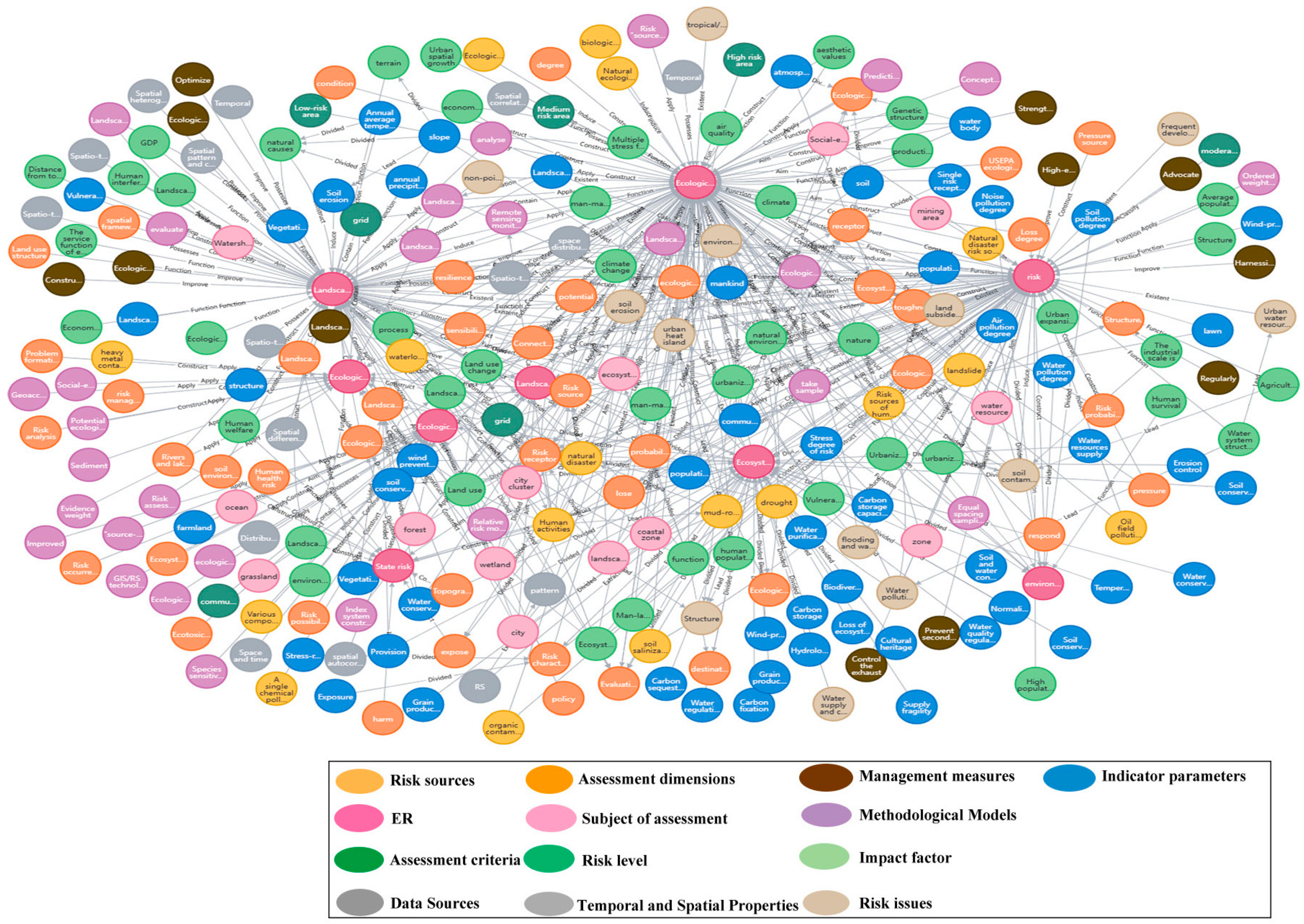
Through combing the KG of the ER, we found that there are big differences in the indicator system frameworks of different evaluation dimensions, and the theoretical approach to ER evaluation has gradually improved from determining the evaluation procedure framework to constructing various quantitative evaluation models. The current integrated evaluation takes into account the probability, intensity, and distributional heterogeneity of the spatial and temporal dimensions of the risk and source analyses. It has evolved from a small-scale evaluation of a single risk source and receptor to a large-scale comprehensive evaluation of multifarious sources of risk and receptors of risk. In this evaluation, we not only paid attention to external coercion, but we also considered the spatial structure, vulnerability, and other attributes of the risk receptor itself. Currently, other academics pay more attention to the anthropogenic sources of the risk and risk receptors that are heavily influenced by human activities, such as urban and rural ecosystems contaminated by heavy metals and persistent organic pollutants.
Furthermore, the main assessment dimensions that appeared more frequently in the KG of the ER were “potential–connectivity–resilience”, “risk sources–risk receptors”, “production–living–ecology”, “landscape pattern–ecological process”, “exposure–sensitivity–adaptive capacity”, and “pressure–state–response”. However, the above assessment dimensions tend to neglect the influence of social systems on ecological and environmental risks when sorting out the indicators. Furthermore, urban ecosystems, typically human–land systems, are the products of mutual trade-offs among multiple elements of socio-ecological systems; complex features, such as the diversification of risk sources and receptors, the determination of administrative boundaries, and the spatial heterogeneity of internal functional partitioning, make it impossible to follow the evaluation dimensions of general regional ecosystems in urban ecosystems (Figure 5). For the study area, which belongs to the Guangdong–Hong Kong–Macao Greater Bay Area, long-term resource exploitation and rapid urban development have changed the land-use composition, structure, and function, which have caused certain disturbances or responses in the region [40]. In response to these issues and in conjunction with the KG of the ER, two characteristic attributes of socio-ecological systems were used as the criterion layer for ER assessment and indicator screening (Table 3). Among them, the social subsystem mainly contains human activities that affect the ER (S1, S2, and S3) and responses to the ER during urban development (S4, S5, and S6), while the ecological subsystem contains natural background quality-threatening ERs (E1, E2, E3, and E4) and background quality responses to the ER (E5, E6, E7, and E8). Therefore, according to the KG of the ER, this study combed the indicators (Figures S1 and S2 in Section S1 of the Supplementary Materials) from the socio-ecological subsystem dimension and constructed an ER assessment framework (Table 3).
4.2. Spatial and Temporal Heterogeneity of ERs
4.2.1. Overall Changes
According to the triangular probability distribution of the weights (Table 4) and the ER evaluation model, the average ERI of each evaluation cell was measured, and the spatial coverage of the ER at the grid scale from 2000 to 2020 was obtained (Figure 6), which showed that the spatial and temporal differentiations were very obvious. Meanwhile, using the natural breakpoint method, the ER was classified into five levels, corresponding to these risk zones: the lowest-risk (ERI ≤ 0.35), lower-risk (0.35 < ERI ≤ 0.45), medium-risk (0.45 < ERI ≤ 0.55), higher-risk (0.55 < ERI ≤ 0.60), and highest-risk areas (ERI > 0.60).
On the time scale, the mean ERI in the study area from 2000 to 2020 was 0.495 (2000), 0.501 (2010), and 0.538 (2020). Moreover, the highest ERI showed an increasing trend (from 0.705 in 2000 to 0.751 in 2020), and the proportion of highest-risk areas gradually increased (7.79% in 2000; 13.99% in 2010; and 20.47% in 2020) (Table 5). Furthermore, the 2000 and 2010 ERIs were dominated by medium- and higher-risk areas, while the 2020 ERI was dominated by higher- and highest-risk areas. Among them, the proportion of high-risk areas (higher- and highest-risk areas) increased by 10.39%, the proportion of low-risk areas (lowest- and lower-risk areas) changed less and remained around 35% overall, while the area proportion of medium-risk areas decreased by 11.16%. In addition, in terms of spatial distribution, the high-risk areas in 2000 were mainly concentrated in the coastal zone of the study area, covering several districts (the Bao’an, Nanshan, Futian, and Luohu Districts); in 2010, they were concentrated in the western part of the study area (the Bao’an, Nanshan, Guangming, and Longhua Districts); and in 2020, the distribution of areas in 2010 was similar, but the final distribution was much more concentrated. The continuous expansion of construction land area in these areas has generated an ecological pressure, leading to a continuous increase in the ER (Figure 6).
Throughout the study period, Moran’s I of the ERI was greater than 0, showing a positive spatial correlation, i.e., the ERs interacted with each other and were spatially similar (Table 6). Overall, Moran’s I of the ERI exhibited an increasing trend over the last 20 years, which indicated that the degrees of spatial aggregation and heterogeneity of ER increased due to socio-economic development and land-use change. The “H-H” agglomeration units (“hotspots”) account for 30.29% (2000), 34.27% (2010), and 32.19% (2020) of the total study area from 2000 to 2020, respectively. In 2000, the “L-L” aggregation unit was mainly concentrated in the southeastern part of the study area, while in 2010 and 2020, the “L-L” aggregation unit showed an expanding trend and was mainly concentrated in the southeastern and northwestern parts of the study area (Figure 5). Overall, the number of “H-H” increased, and then decreased, with an overall decreasing trend, while the number of “L-L” increased. The decrease in the number of non-significant spatial aggregation units indicates more local spatial aggregation of the ERs.
4.2.2. Analysis of Subsystem Changes
First, we analyzed the social subsystem. The distribution of the risk in the social subsystem for the period 2000–2020 gradually decreased, and the maximum, mean, and minimum values increased by varying degrees. The increase in the maximum and minimum values was smaller, with the maximum value increasing from 0.413 (2000) to 0.445 (2020) and the minimum value increasing from 0.101 (2000) to 0.129 (2020). Between 2000 and 2010, the spatial distribution of the risk in the social subsystem was slightly limited, with high values mainly found in the southeastern part of the study area and low values mainly found in the core development areas of the districts and counties; the spatial distribution of the risk in the social subsystem in 2020 was significantly different from that in the previous two periods, with gradually fewer low-value areas (more concentrated in the southwest of the study area) and gradually more high-value areas (Figure 7).
The overall mean indicator values in the social subsystem showed varying degrees of change over the period 2000–2020. For the positive indicators (S1, S2, and S3), the mean valued showed fluctuating changes. The mean values of S1 were 0.194 (2000), 0.196 (2010), and 0.192 (2020), while the mean values of S3 were 0.161 (2000), 0.218 (2010), and 0.148 (2020). On the other hand, the mean values of S2 increased, with mean values of 0.132 (2000), 0.138 (2010), and 0.165 (2020). For the negative indicators (S4, S5, and S6), the changes in the mean values of S5 and S6 were larger. The mean values for S5 were 0.466 (2000), 0.487 (2010), and 0.856 (2020); for S6, they were 0.884 (2000), 0.829 (2010), and 0.941 (2020). It should be added that with socio-economic and regional development, the GDP (S5) and the density of parklands (S6) have increased substantially, especially in the southwestern part of the study area, but the disparity between regional development also increased, and there are many low-value zones, which make the overall value after standardization high, and this is what leads to an increased risk in the social subsystems (Figure 7).
Second, we analyzed the ecological subsystem. The distribution of the risk in the ecological subsystem from 2000 to 2020 gradually widened, with the maximum, mean, and minimum values showing different degrees of change. Among them, the mean of the risk value of the ecological subsystem decreased a little, with the mean value decreasing from 0.280 (2000) to 0.278 (2020), whereas the maximum and minimum values showed some changes, with the maximum value increasing from 0.410 (2000) to 0.428 (2020) and the minimum value decreasing from 0.144 (2000) to 0.119 (2020). The spatial distribution of the risk in the ecological subsystem from 2000 to 2020 had a high degree of similarity, with the high-value areas mainly concentrated in the western, central, and northeastern parts of the study area, while the low-value areas were mainly concentrated in the southeastern part of the study area (Figure 7).
The overall mean values of the indicators in the ecological subsystem also showed different degrees of change from 2000 to 2020. For the positive indicators (E1, E2, E3, and E4), the changes in their mean values were small. The mean values of E2 decreased: 0.593 (2000), 0.527 (2010), and 0.504 (2020); the mean values of E3 decreased in a fluctuating manner: 0.472 (2000), 0.409 (2010), and 0.452 (2020); and the mean values of the other two indicators (E1 and E4) were stable. Therefore, to a certain extent, E2 and E3 contributed more to the assessment of the results. For the negative indicators (E5, E6, E7, and E8), the magnitude of change in their means was large. The change in the mean value of E6 was not significant, while the means of E5, E7, and E8 increased. The mean values of E5 were 0.345 (2000), 0.367 (2010), and 0.375 (2020); the mean values of E8 were 0.502 (2000), 0.545 (2010), and 0.565 (2020); and the mean values of E7 were 0.432 (2000), 0.452 (2010), and 0.481 (2020). Therefore, to some extent, E5, E7, and E8 contributed more to the assessed outcomes (Figure 7).
4.2.3. Uncertainty Analysis of ER Assessment Results in the Study Area
In the Monte Carlo simulation, the uncertainty of the weights was gradually transferred to the assessment results during calculation. As a result, there was uncertainty in this evaluation result. Moreover, the ERI was calculated using the ecological and social subsystem risk indices, and the uncertainty was directly transferred through them.
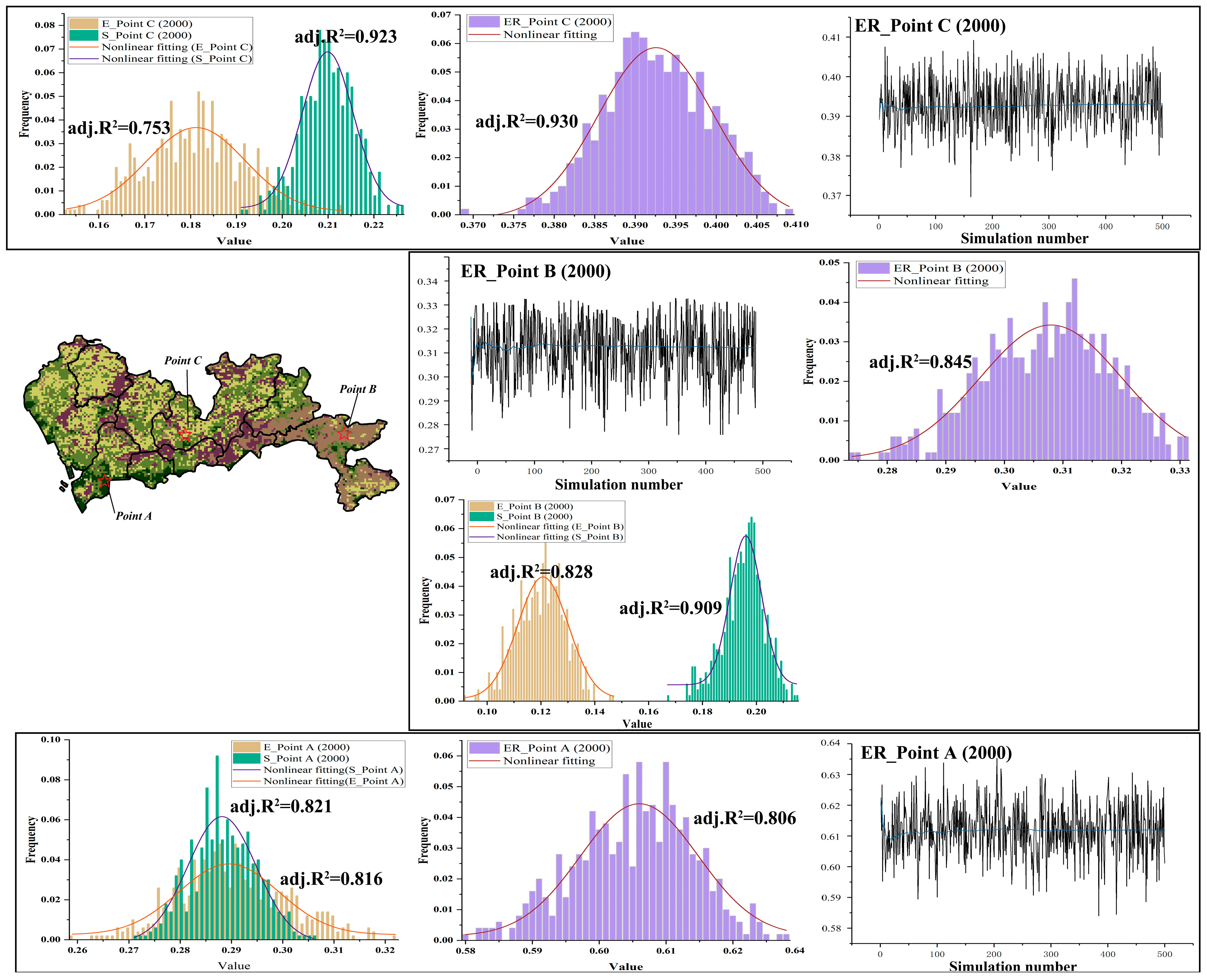
The areas with the highest ERI, as shown in the assessment results, were mainly located in the southwest and northwest of the study area (point A). This is because the area rapidly developed and has weak ecosystem services, which is one of the reasons for the high-level ERI. The ERI indices for point A ranged from 0.58~0.64 (2000) to 0.47~0.53 (2010) and 0.65~0.69 (2020), and their mean values for 500 iterations were 0.614 (2000), 0.519 (2010), and 0.675 (2020), respectively. The adj. R2 values were 0.806 (2000), 0.805 (2010), and 0.907 (2020), respectively. In addition, the risk indices for the ecological and social subsystems of point A also showed uncertainty. The mean values of the 500 iterations of the risk index for the ecological subsystem of point A were 0.309 (2000) (range: 0.27–0.33), 0.312 (2010) (range: 0.27–0.33), and 0.359 (2020) (range: 0.32–0.38). Their adj. R2 values were 0.816 (2000), 0.831 (2010), and 0.842 (2020), respectively. In contrast, the averages of 500 iterations of the risk index for the social subsystem at point A were 0.298 (2000) (range: 0.28–0.32), 0.225 (2010) (range: 0.19–0.24), and 0.312 (2020) (range: 0.31–0.32). Their adj. R2 values were 0.821 (2000), 0.866 (2010), and 0.913 (2020) (Figure 8 and Figure S3 in Section S2 of the Supplementary Materials), respectively.
The assessment results show that the lower areas of the ERI were mainly located in the southeastern part of the study area (point B); this is because this area is used for ecological purposes, the landscape type is dominated by woodland, the ecosystem service function level is high, and human activities cause minimal impacts, which was also one of the reasons for the reduction in the ERI. The ERIs for point B were 0.27~0.34 (2000), 0.32~0.40 (2010), and 0.35~0.41 (2020); their means of 500 iterations were 0.314 (2000), 0.365 (2010), and 0.387 (2020); and the adj. R2 values were 0.845 (2000), 0.747 (2010), and 0.751 (2020), respectively. Meanwhile, the mean values of 500 iterations of the risk index for the ecological subsystem at point B were 0.133 (2000) (range: 0.09–0.15), 0.165 (2010) (range: 0.14–0.19), and 0.175 (2020) (range: 0.14–0.20). The adj. R2 values were 0.828 (2000), 0.842 (2010), and 0.846 (2020). The averages of 500 iterations of the risk index for the ecological subsystem at point B were 0.193 (2000) (range: 0.17–0.22), 0.198 (2010) (range: 0.17–0.22), and 0.213 (2020) (range: 0.18–0.23), respectively. The adj. R2 values were 0.909 (2000), 0.865 (2010), and 0.917 (2020) (Figure 8 and Figure S3 in Section S2 of the Supplementary Materials), respectively.
The results of the assessment showed that the areas with a medium ERI were mainly located in the central part of the study area (point C). This is because this area is a peripheral area for urban development, where ecosystem service functioning and human activities were some of the causes affecting the ER. The ERIs for point C were 0.37~0.41 (2000), 0.44~0.50 (2010), and 0.55~0.60 (2020); their means of 500 iterations were 0.394 (2000), 0.474 (2010), and 0.581 (2020); and their adj. R2 values were 0.930 (2000), 0.814 (2010), and 0.867 (2020), respectively. Meanwhile, the averages of 500 iterations of the risk index for the ecological subsystem at point C were 0.186 (2000) (range: 0.15–0.21), 0.287 (2010) (range: 0.24–0.30), and 0.305 (2020) (range: 0.27–0.33). The adj. R2 values were 0.753 (2000), 0.839 (2010), and 0.817 (2020), respectively. In contrast, the averages of 500 iterations of the risk index for the social subsystem at point C were 0.211 (2000) (range: 0.201–0.253), 0.209 (2010) (range: 0.18–0.22), and 0.264 (2020) (range: 0.24–0.28). The adj. R2 values were 0.923 (2000), 0.922 (2010), and 0.894 (2020) (Figure 8 and Figure S3 in Section S2 of the Supplementary Materials), respectively.
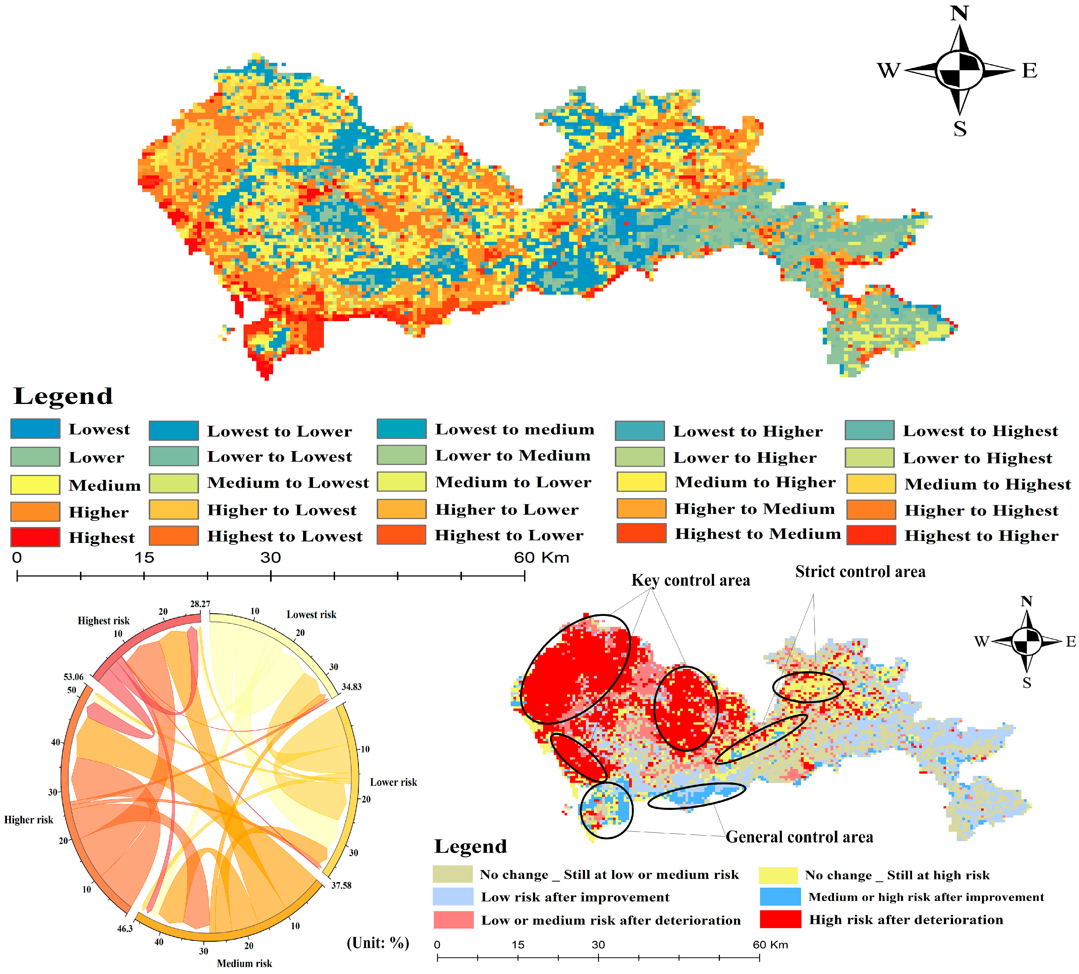
4.3. Precaution Partitions to Circumvent ER
ER evaluation is the process of collecting, collating, and expressing scientific information, which is conducive for environmental decision making [13]. In addition, in the context of the development of information technology, the promotion of accurate ER knowledge is not only an intrinsic requirement for ecological civilization construction, but it is necessary for the promotion of high-quality sustainable development in the region [41]. In this study, the rank of each ER in the study area from 2000 to 2020 was obtained by superimposing the distribution graphs. As shown in Figure 9, the top three areas transferred were: medium risk to higher risk (9.66% of the total area), higher risk to the highest risk (9.55% of the total area), and the lowest risk to lower risk (7.06% of the total area). It can be seen that most of the ER grades in the study area shifted from low to high grades, and the ER was intensified, which, in turn, led to serious ecological problems. In addition, according to the needs of ER prevention and control, the study area was divided into key, strict, and general control areas via the process of ER level transfer, as described below.
- (1)
- The key control area of the ER: This area is mainly where the ER shifted from a low to a high grade, and the ER deteriorated. The key control areas are mainly located in the western part of the study area, where ecological land use is scarce and scattered, and construction land use accounts for a large proportion and covers an ever-expanding area, resulting in ecological and environmental pressures; the ER continues to rise. In response to such problems, our future work will focus on improving land use, rationalizing industrial arrangements, and transforming the mode of economic development. Furthermore, establishing a proper ecological compensation system will be essential to promote the natural environment and sustainable socio-economic development [42].
- (2)
- The strict control zone of the ER: This zone is mainly where the grade of ER has not shifted, and the ER has not improved significantly. It should be noted that the strict control zone is targeted at areas with high ER levels (highest- and higher-risk areas). Strict control zones are mainly located in the southwest and southeast of the study area and should play a leading role in territorial spatial planning, where the incremental development of construction land is accompanied by the renewal of stock, to minimize the negative impacts on the ecology and maintain the current level of ecological risk, while promoting economic development [43]. In addition, it is essential to improve the capacity and quality of environmental facilities to make full use of their functions and potential applications, such as the development of ecotourism, the improvement of nature reserves, etc. This management model promotes both the ecological protection of the specific environment and the growth of the regional economy, creating a virtuous circle of benefits.
- (3)
- The general control area of the ER: This area is mainly where the ER shifted from higher to lower grades, with some improvement in the ER. It should be added that the general control area focuses more on the areas where an improvement in rank is not significant. The general control zone is mainly located in the central part of the study area, with a small amount in the southeastern and western parts of the study area. To mitigate some of the negative impacts associated with socio-economic development, targeted ecological protection and restoration should be carried out in this region. In addition, the ecological advantages of the site need to be maintained to prevent further deterioration of the ER, while strengthening the infrastructure [44].
Figure 9.
Risk level transfer of the ER and precaution partitions.
5. Discussion
5.1. Exploration of the ER Assessment Framework
Firstly, with the rapid development of big data and artificial intelligence technologies, more and more research has been devoted to the development of knowledge-driven ER assessments, which monitor and explain the development of ERs and produce large amounts of academic data [45]. However, the existing research results [46] have tried to show the feasibility and effectiveness of the KG in terms of its application in the ecological field [32] in multiple tasks and referenced a typical research framework from construction to application. Therefore, by constructing the KG of the ER, this study comprehensively and deeply grasps the interrelationships and evolutionary processes between various elements in the field of ER and provides effective data and decision-making support for the establishment of an ER evaluation index system.
Through the KG of the ER, it was found that when the ER is assessed for ecological categories, such as wetlands [47], rivers [13], and lakes [48], the assessment framework is mainly constructed from the risk source–risk receptor perspective, focusing on the impact of the natural ecological environment on the ER [16]; when the ER is assessed for ecological categories, such as croplands [6] and cities [49], the assessment framework is mainly constructed using the dimensions of disturbance and exposure of the ER, taking into account the impact of natural ecology and human activities [17]. Although the above assessment frameworks can effectively characterize the ER, they often confuse the classification or attribution of the indicators. To address this problem, this study considers the urban system, as a typical complex land-use system, as a product of multiple trade-offs between the social and ecological systems [50], and the urbanization process exacerbates the conflicts between the ecological environment and socio-economic development. Therefore, this study introduces the socio-ecological system framework [51], which is conducive to elucidating the interactions between the social and ecological subsystems and revealing the non-linear, multi-level constitutive characteristics of the system.
Finally, human or economic activities on urban land pose a challenge to the ER in fast-growing cities [13]. These urban systems are highly vulnerable and face multiple threats [3,52]. The concentration of people, industries, and infrastructure in urban areas increases the risk of natural hazards, which highlights regional differences in ER resilience [45]. This study area is a highly urbanized region, which focuses more on the disturbance or response to ERs generated during urban development. Therefore, this study screens the dimensional indicators of ecosystem service function (E5–E8), climate (E3), human activities (S1), urban facility development (S2, S3, S5, and S6), etc. In conclusion, the ER assessment indicators constructed through the KG in this study overlap with the findings of Na et al. [41], Guo et al. [44], Zhao et al. [2], etc.
5.2. Exploration of ER Assessment Methods and Results
Establishing an ER assessment method that is applicable to cities has been a research hotspot in this field [53]. Compared with traditional ER assessments, the method in this study can better determine the weights of indicators. The key to the quantification of ERs is to construct reasonable and appropriate weights, and the different distributions of the weights of each indicator will directly affect the evaluation result [25]. In the existing research results, more methods, such as the entropy value approach [54], analytic hierarchy process (AHP) [55], fuzzy comprehensive evaluation (FCE) [17], etc., are used to determine the weights of the indicators. However, among the many weighting methods, how does one choose the appropriate method to truly reflect the level of ER? To address this problem, this study introduces a Monte Carlo simulation model to simulate the weights for ER evaluation in the study area, while the impact of the uncertainty of the weights on the evaluation results was analyzed. Compared with subjective weighting, objective weighting, and combined subjective–objective weighting methods [56], this methodology effectively simulates the transfer of uncertainty from the indicator weights to the quantitative results, and at the same time, can integrate ER uncertainty and spatial information, making the ERI quantitative results more objective and reliable.
Secondly, based on the quantitative results of the ER from 2000 to 2020, the overall risk level increased. Among them, the average value of the social subsystem risk index is higher, and its change is more significant, which is also the key factor leading to the increase in the risk level. The areas with high risk levels are more concentrated in the areas with more human activity or dispersed ecological lands, which affects the final quantification results. Furthermore, the areas with many ecosystem services are too fragile, so the social subsystems are at a higher risk. Therefore, the rational coordination of social and ecological subsystems is still an important step to avoid these risks. In addition, based on the results of the Monte Carlo simulation operations, we selected three sample sites (A–C) to analyze the ER levels and their uncertainties (95% confidence intervals) and found that the predominantly impervious region with a high level of urban development has high ERIs; the region with a high level of vegetation cover and fewer urban development activities has low ERIs; and the region between the former and the latter levels has medium ERIs. For the urban systems, the ERI is highly correlated with the quality of the ecosystem and the level of urban development [57]. In conclusion, the methodological system constructed shows a lower overall risk level in areas with ecological land use or less development and fewer construction activities than that in the core areas of urban construction and development, which is somewhat similar to the pattern described by Lu et al. [13] and Shen et al. [58].
5.3. Shortcomings and Prospects
This study examines the level of ER in Shenzhen over the last 20 years at the grid scale and develops improvement measures based on the zoning scheme. Compared with the existing research results, there have been some improvements in the judgment perspective and research methods. However, there are some shortcomings. First, although this study combines the social and ecological dimensions to construct the evaluation index system of the ER based on a KG, the index system can only alleviate the problem of inconsistency in the existence of evaluation indexes to a certain extent, and the results of the study are still unavoidably affected by the indexes. Second, this study quantifies the uncertainty of the ER assessment process, but lacks an in-depth exploration of the division of ER levels and the driving mechanism in the risk evolution process. Finally, this study mainly focuses on the evolution process of ER ranking when determining the zoning scheme, but the management measures still need to be improved.
Given these shortcomings, this study still needs to explore many aspects: for example, the evaluation index system of the ER and its processing method still deserve in-depth analysis and selection; to determine whether there is a more scientific and effective method for ER rating; and the natural breakpoint method of GIS also deserves to be investigated. Additionally, we must determine whether the spatial resolution of the other data can be further improved, and so on. This study will further improve the evaluation framework of ER, better reflect the interaction between the ecological and socio-economic factors, and formulate more integrated and comprehensive zoning programs and management measures. It is believed that as the research progresses, more in-depth evaluation mechanisms and methods will be gradually established and improved to provide more scientific guidance for the realization of regional high-quality development.
6. Conclusions
Based on the KG of the ER, this study constructs the indicator system of ER in the study area from two dimensions: social and ecological. Furthermore, the study quantifies the uncertainty due to the determination of weights with the help of the Monte Carlo simulation model, divides different levels of risk control areas according to the quantification results, and puts forward risk avoidance measures in a targeted manner. The conclusions are as follows:
- (1)
- The average values of ERI from 2000 to 2020 are 0.495 (2000), 0.501 (2010), and 0.538 (2020), and its highest value shows an increasing trend. In terms of spatial distribution, the high-risk area in 2000 was mainly concentrated in the coastal zone of the study area, and the areas distributed in 2010 and 2020 had some similarity, but the distribution results in 2020 were more concentrated. In addition, the mean value of the risk index of the social subsystem was higher than that of the ecological subsystem in the ER’s assessment system.
- (2)
- In order to better elucidate the uncertainty in the ER assessment, three sample sites (A–C) were selected to describe the means and intervals of change of their ERI, risk index of ecological subsystem, and risk index of social subsystem from 2000–2020. To some extent, it shows the uncertainty generated by different weights of indicators and its transmission process.
- (3)
- Based on the quantitative results of ER and its transfer characteristics in the study area from 2000 to 2020, it was divided into key control areas, strict control areas, and general control areas of ER, and targeted improvement measures were proposed. Although the study area is a high-speed urbanization area, particular attention is paid to guaranteeing the coordination of the ecological and social subsystems.
Supplementary Materials
The following supporting information can be downloaded at: https://www.mdpi.com/article/10.3390/su16020909/s1, Figure S1: Results after standardization of indicators covered by ecological subsystems. Figure S2: Results after standardization of the indicators covered by the social subsystems. Figure S3: Uncertainty of sample points in the ER and its subsystems (2010 and 2020).
Author Contributions
Methodology, Y.Y.; Formal analysis, X.Z.; Investigation, X.Z.; Writing—review & editing, Y.Y.; Supervision, Y.Y.; Funding acquisition, Y.Y. All authors have read and agreed to the published version of the manuscript.
Funding
This research was financially supported by the Open Fund of Key Laboratory of Urban Land Resources Monitoring and Simulation, Ministry of Natural Resources (No. KF-2022-07-011), and the Youth Fund for Humanities and Social Sciences, Ministry of Education (No. 23YJC630212). The authors would like to extend their appreciation to all the anonymous reviewers and editors for their constructive comments that improved the study.
Institutional Review Board Statement
Not applicable.
Informed Consent Statement
Not applicable.
Data Availability Statement
The data presented in this study are available on request from the corresponding author.
Conflicts of Interest
The authors declare no conflict of interest.
References
- Li, W.; An, M.; Wu, H.; An, H.; Huang, J.; Khanal, R. The local coupling and telecoupling of urbanization and ecological environment quality based on multisource remote sensing data. J. Environ. Manag. 2023, 327, 116921. [Google Scholar] [CrossRef] [PubMed]
- Zhao, Y.; Li, B.; Ni, J.; Liu, L.; Niu, X.; Liu, J.; Shao, J.; Du, S.; Chu, L.; Jin, J.; et al. Global spatial and temporal patterns of fine particulate concentrations and exposure risk assessment in the context of SDG indicator 11.6.2. Ecol. Indic. 2023, 155, 111031. [Google Scholar] [CrossRef]
- Gao, L.; Tao, F.; Liu, R.; Wang, Z.; Leng, H.; Zhou, T. Multi-scenario simulation and ecological risk analysis of land use based on the PLUS model: A case study of Nanjing. Sustain. Cities Soc. 2022, 85, 104055. [Google Scholar] [CrossRef]
- Wu, J.; Zhu, Q.; Qiao, N.; Wang, Z.; Sha, W.; Luo, K.; Wang, H.; Feng, Z. Ecological risk assessment of coal mine area based on “source-sink” landscape theory—A case study of Pingshuo mining area. J. Clean. Prod. 2021, 295, 126371. [Google Scholar] [CrossRef]
- Cai, X.; Li, Z.; Liang, Y. Tempo-spatial changes of ecological vulnerability in the arid area based on ordered weighted average model. Ecol. Indic. 2021, 133, 108398. [Google Scholar] [CrossRef]
- Qiu, M.; Fu, M.; Zhang, Z.; Fu, S.; Yuan, C. Assessing the ecological risk of croplands in loess drylands by combining environmental disturbance with ecosystem vulnerability. J. Environ. Manag. 2023, 347, 119231. [Google Scholar] [CrossRef]
- Bhuiyan, M.A.H.; Karmaker, S.C.; Doza, B.; Rakib, A.; Saha, B.B. Enrichment, sources and ecological risk mapping of heavy metals in agricultural soils of dhaka district employing SOM, PMF and GIS methods. Chemosphere 2021, 263, 128339. [Google Scholar] [CrossRef]
- Jiao, C.; Chen, L.; Sun, C.; Jiang, Y.; Zhai, L.; Liu, H.; Shen, Z. Evaluating national ecological risk of agricultural pesticides from 2004 to 2017 in China. Environ. Pollut. 2019, 259, 113778. [Google Scholar] [CrossRef]
- Sharma, T.; Vittal, H.; Karmakar, S.; Ghosh, S. Increasing agricultural risk to hydro-climatic extremes in India. Environ. Res. Lett. 2020, 15, 034010. [Google Scholar] [CrossRef]
- Yu, J.; Tang, B.; Chen, Y.; Zhang, L.; Nie, Y.; Deng, W. Landscape ecological risk assessment and ecological security pattern construction in landscape resource-based city: A case study of Zhangjiajie City. Acta Ecol. Sin. 2022, 42, 1290–1299, (In Chinese with English abstract). [Google Scholar]
- Wu, Z.; Lin, C.; Shao, H.; Feng, X.; Chen, X.; Wang, S. Ecological risk assessment and difference analysis of pit ponds under different ecological service functions—A case study of Jianghuai ecological Economic Zone. Ecol. Indic. 2021, 129, 107860. [Google Scholar] [CrossRef]
- Xu, W.; Wang, J.; Zhang, M.; Li, S. Construction of landscape ecological network based on landscape ecological risk assessment in a large-scale opencast coal mine area. J. Clean. Prod. 2021, 286, 125523. [Google Scholar] [CrossRef]
- Lu, Y.; Li, Y.; Fang, G.; Deng, M.; Sun, C. Ecological risk assessment and management for riverfront development along the Yangtze River in Jiangsu Province, China. Ecol. Indic. 2023, 155, 111075. [Google Scholar] [CrossRef]
- Vezi, M.; Downs, C.; Wepener, V.; O’Brien, G. Application of the relative risk model for evaluation of ecological risk in selected river dominated estuaries in KwaZulu-Natal, South Africa. Ocean Coast. Manag. 2019, 185, 105035. [Google Scholar] [CrossRef]
- Ju, H.; Niu, C.; Zhang, S.; Jiang, W.; Zhang, Z.; Zhang, X.; Yang, Z.; Cui, Y. Spatiotemporal patterns and modifiable areal unit problems of the landscape ecological risk in coastal areas: A case study of the Shandong Peninsula, China. J. Clean. Prod. 2021, 310, 127522. [Google Scholar] [CrossRef]
- Proshad, R.; Kormoker, T.; Al, M.A.; Islam, S.; Khadka, S.; Idris, A.M. Receptor model-based source apportionment and ecological risk of metals in sediments of an urban river in Bangladesh. J. Hazard. Mater. 2022, 423, 127030. [Google Scholar] [CrossRef] [PubMed]
- Qian, L.; Shi, Y.; Xu, Q.; Zhou, X.; Li, X.; Shao, X.; Xu, C.; Liang, R. A prospective ecological risk assessment method based on exposure and ecological scenarios (ERA-EES) to determine soil ecological risks around metal mining areas. Sci. Total. Environ. 2023, 901, 166371. [Google Scholar] [CrossRef]
- Liu, C.; Zhang, X.; Xu, Y.; Xiang, B.; Gan, L.; Shu, Y. Knowledge graph for maritime pollution regulations based on deep learning methods. Ocean Coast. Manag. 2023, 242, 106679. [Google Scholar] [CrossRef]
- Li, J.; Sun, A.; Han, J.; Li, C. A Survey on Deep Learning for Named Entity Recognition. IEEE Trans. Knowl. Data Eng. 2022, 34, 50–70. [Google Scholar] [CrossRef]
- Singh, J.; Kumaraswamidhas, L.; Bura, N.; Sharma, N.D. A Monte Carlo simulation investigation on the effect of the probability distribution of input quantities on the effective area of a pressure balance and its uncertainty. Measurement 2021, 172, 108853. [Google Scholar] [CrossRef]
- Roszkowski, M. Modelling doctoral dissertations in Wikidata knowledge graph: Selected issues. J. Acad. Libr. 2022, 49, 102658. [Google Scholar] [CrossRef]
- Saad, M.; Zhang, Y.; Tian, J.; Jia, J. A graph database for life cycle inventory using Neo4j. J. Clean. Prod. 2023, 393, 136344. [Google Scholar] [CrossRef]
- Han, F.; Deng, Y.; Liu, Q.; Zhou, Y.; Wang, J.; Huang, Y.; Zhang, Q.; Bian, J. Construction and application of the knowledge graph method in management of soil pollution in contaminated sites: A case study in South China. J. Environ. Manag. 2022, 319, 115685. [Google Scholar] [CrossRef] [PubMed]
- Wang, X.; Meng, L.; Wang, X.; Wang, Q. The construction of environmental-policy-enterprise knowledge graph based on PTA model and PSA model. Resour. Conserv. Recycl. Adv. 2021, 12, 200057. [Google Scholar] [CrossRef]
- Yang, Y.J.; Song, G.; Lu, S. Assessment of land ecosystem health with Monte Carlo simulation: A case study in Qiqihaer, China. J. Clean. Prod. 2020, 250, 119522. [Google Scholar] [CrossRef]
- Jia, C.; Altaf, A.R.; Li, F.; Ashraf, I.; Zafar, Z.; Nadeem, A.A. Comprehensive assessment on groundwater quality, pollution characteristics, and ecological health risks under seasonal thaws: Spatial insights with Monte Carlo simulations. Groundw. Sustain. Dev. 2023, 22, 100952. [Google Scholar] [CrossRef]
- Barandas, M.; Famiglini, L.; Campagner, A.; Folgado, D.; Simão, R.; Cabitza, F.; Gamboa, H. Evaluation of uncertainty quantification methods in multi-label classification: A case study with automatic diagnosis of electrocardiogram. Inf. Fusion 2023, 101, 101978. [Google Scholar] [CrossRef]
- Zhao, J.; Pan, B. Uncertainty quantification for 3D digital image correlation displacement measurements using Monte Carlo method. Opt. Lasers Eng. 2023, 170, 107777. [Google Scholar] [CrossRef]
- Rullens, V.; Stephenson, F.; Hewitt, J.E.; Clark, D.E.; Pilditch, C.A.; Thrush, S.F.; Ellis, J.I. The impact of cumulative stressor effects on uncertainty and ecological risk. Sci. Total Environ. 2022, 842, 156877. [Google Scholar] [CrossRef]
- Zhou, Y.; Zheng, Z.; Wu, Z.; Guo, C.; Chen, Y. Construction and evaluation of ecological networks in highly urbanised regions: A case study of the Guangdong-Hong Kong-Macao greater Bay Area, China. Ecol. Indic. 2023, 152, 110336. [Google Scholar] [CrossRef]
- Wang, Z.H.; Yang, X.M.; Zhou, C.H. Geographic Knowledge Graph for Remote Sensing Big Data. J. Geo-Inf. Sci. 2021, 23, 16–28. [Google Scholar] [CrossRef]
- Wang, T.Y.; Meng, X.L.; Zhang, H. Knowledge Graph Construction Method in the Ecology and Environment Field. Geospat. Inf. 2023, 21, 14–19, (In Chinese with English abstract). [Google Scholar]
- Deng, L.; Qi, P.H.; Liu, Z.H.; Li, J.; Tang, J. BGPNRE: A BERT-based Global Pointer Network for Named Entity-Relation Joint Extraction Method. Comput. Sci. 2023, 50, 42–48. [Google Scholar] [CrossRef]
- Yao, Y.; Yang, F. Chinese Keyword Extraction Method Combining Knowledge Graph and Pre-training Model. Comput. Sci. 2022, 49, 243–251. [Google Scholar] [CrossRef]
- Abarna, S.; Sheeba, J.; Devaneyan, S.P. An ensemble model for idioms and literal text classification using knowledge-enabled BERT in deep learning. Meas. Sens. 2022, 24, 100434. [Google Scholar] [CrossRef]
- Zhang, Y.; Li, J.; Xin, Y.; Zhao, X.; Liu, Y. A Model for Chinese Named Entity Recognition Based on Global Pointer and Adversarial Learning. Chin. J. Electron. 2023, 32, 854–867. [Google Scholar] [CrossRef]
- Wu, S.S.; Zhou, A.L.; Xie, N.F. Construction of visualization domain-specific knowledge graph of crop diseases and pests based on deep learning. Trans. Chin. Soc. Agric. Eng. 2000, 36, 177–185. [Google Scholar] [CrossRef]
- Singh, K.; Lytra, I.; Radhakrishna, A.S.; Shekarpour, S.; Vidal, M.-E.; Lehmann, J. No one is perfect: Analysing the performance of question answering components over the DBpedia knowledge graph. J. Web Semant. 2020, 65, 100594. [Google Scholar] [CrossRef]
- Zhang, F.; Liu, X.; Zhang, J.; Wu, R.; Ma, Q.; Chen, Y. Ecological vulnerability assessment based on multi-sources data and SD model in Yinma River Basin, China. Ecol. Model. 2017, 349, 41–50. [Google Scholar] [CrossRef]
- Zhang, W.; Liu, G.; Yang, Z. Urban agglomeration ecological risk transfer model based on Bayesian and ecological network. Resour. Conserv. Recycl. 2020, 161, 105006. [Google Scholar] [CrossRef]
- Na, L.; Zhao, Y.; Feng, C.-C.; Guo, L. Regional ecological risk assessment based on multi-scenario simulation of land use changes and ecosystem service values in Inner Mongolia, China. Ecol. Indic. 2023, 155, 111013. [Google Scholar] [CrossRef]
- Cueva, J.; Yakouchenkova, I.A.; Fröhlich, K.; Dermann, A.F.; Dermann, F.; Köhler, M.; Grossmann, J.; Meier, W.; Bauhus, J.; Schröder, D.; et al. Synergies and trade-offs in ecosystem services from urban and peri-urban forests and their implication to sustainable city design and planning. Sustain. Cities Soc. 2022, 82, 103903. [Google Scholar] [CrossRef]
- Liu, Z.; Huang, Q.; Zhou, Y.; Sun, X. Spatial identification of restored priority areas based on ecosystem service bundles and urbanization effects in a megalopolis area. J. Environ. Manag. 2022, 308, 114627. [Google Scholar] [CrossRef] [PubMed]
- Guo, H.; Cai, Y.; Li, B.; Wan, H.; Yang, Z. An improved approach for evaluating landscape ecological risks and exploring its coupling coordination with ecosystem services. J. Environ. Manag. 2023, 348, 119277. [Google Scholar] [CrossRef] [PubMed]
- Zhang, W.; Liu, G.; Ghisellini, P.; Yang, Z. Ecological risk and resilient regulation shifting from city to urban agglomeration: A review. Environ. Impact Assess. Rev. 2024, 105, 107386. [Google Scholar] [CrossRef]
- Xie, X.X.; Chen, M.Q.; Tian, Y. Land Ecological Research Hotspots in Recent 20 Years in China and Its Prospect: A Knowledge Map Analysis based on the Ucinet. China Land Sci. 2018, 32, 88–96, (In Chinese with English abstract). [Google Scholar]
- Ashraf, A.; Khalid, A.; Khan, I.; Yuke, Z.; Zhigang, C.; Zhaoxue, T.; Leite, F.; Xuehua, L. Integrated multiphase ecological risk assessment of heavy metals for migratory water birds in wetland ecosystem: A case study of Dongzhangwu Wetland, China. Sci. Total Environ. 2023, 889, 164102. [Google Scholar] [CrossRef]
- Lu, H.; Fu, Z.; Tong, Y.; Xiang, S.; Sun, Y.; Wu, F. Combined pollution characteristics and ecological risks of multi-pollutants in Poyang Lake. Environ. Pollut. 2024, 342, 123116. [Google Scholar] [CrossRef]
- Lin, X.; Wang, Z. Landscape ecological risk assessment and its driving factors of multi-mountainous city. Ecol. Indic. 2023, 146, 109823. [Google Scholar] [CrossRef]
- Hou, Y.; Liu, Y.; Zeng, H. Assessment of urban ecosystem condition and ecosystem services in Shenzhen based on the MAES analysis framework. Ecol. Indic. 2023, 155, 110962. [Google Scholar] [CrossRef]
- Liu, R.; Zhang, L.; Tang, Y.; Jiang, Y. Understanding and evaluating the resilience of rural human settlements with a social-ecological system framework: The case of Chongqing Municipality, China. Land Use Policy 2024, 136, 106966. [Google Scholar] [CrossRef]
- Qu, Y.; Zong, H.; Su, D.; Ping, Z.; Guan, M. Land Use Change and Its Impact on Landscape Ecological Risk in Typical Areas of the Yellow River Basin in China. Int. J. Environ. Res. Public Health 2021, 18, 11301. [Google Scholar] [CrossRef] [PubMed]
- Zhang, W.; Liu, G.; Gonella, F.; Xu, L.; Yang, Z. Research on collaborative management and optimization of ecological risks in urban agglomeration. J. Clean. Prod. 2022, 372, 133735. [Google Scholar] [CrossRef]
- Zhang, H.; Liu, Y.; Li, X.; Feng, R.; Gong, Y.; Jiang, Y.; Guan, X.; Li, S. Combing remote sensing information entropy and machine learning for ecological environment assessment of Hefei-Nanjing-Hangzhou region, China. J. Environ. Manag. 2023, 325, 116533. [Google Scholar] [CrossRef] [PubMed]
- Li, Y.; Lu, C.; Liu, G.; Chen, Y.; Zhang, Y.; Wu, C.; Liu, B.; Shu, L. Risk assessment of wetland degradation in the Xiong’an New Area based on AHP-EWM-ICT method. Ecol. Indic. 2023, 153, 110443. [Google Scholar] [CrossRef]
- Gong, J.; Jin, T.; Cao, E.; Wang, S.; Yan, L. Is ecological vulnerability assessment based on the VSD model and AHP-Entropy method useful for loessial forest landscape protection and adaptative management? A case study of Ziwuling Mountain Region, China. Ecol. Indic. 2022, 143, 109379. [Google Scholar] [CrossRef]
- Zeng, C.; He, J.; He, Q.; Mao, Y.; Yu, B. Assessment of Land Use Pattern and Landscape Ecological Risk in the Chengdu-Chongqing Economic Circle, Southwestern China. Land 2022, 11, 659. [Google Scholar] [CrossRef]
- Shen, W.; Zhang, J.; Wang, K.; Zhang, Z. Identifying the spatio-temporal dynamics of regional ecological risk based on Google Earth Engine: A case study from Loess Plateau, China. Sci. Total Environ. 2023, 873, 162346. [Google Scholar] [CrossRef]
Figure 1.
Geographical location of the study area.
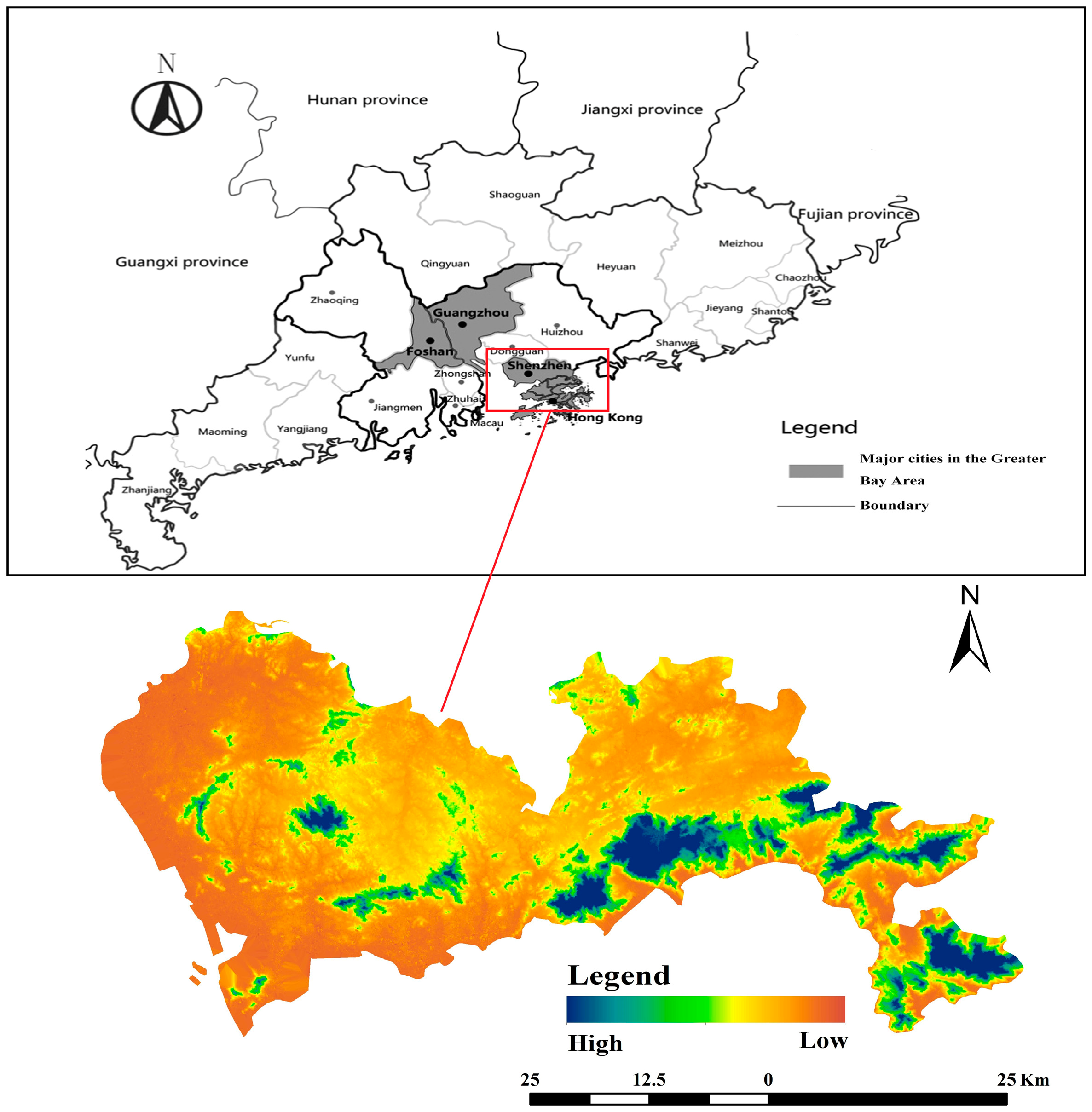
Figure 2.
Technology Roadmap.
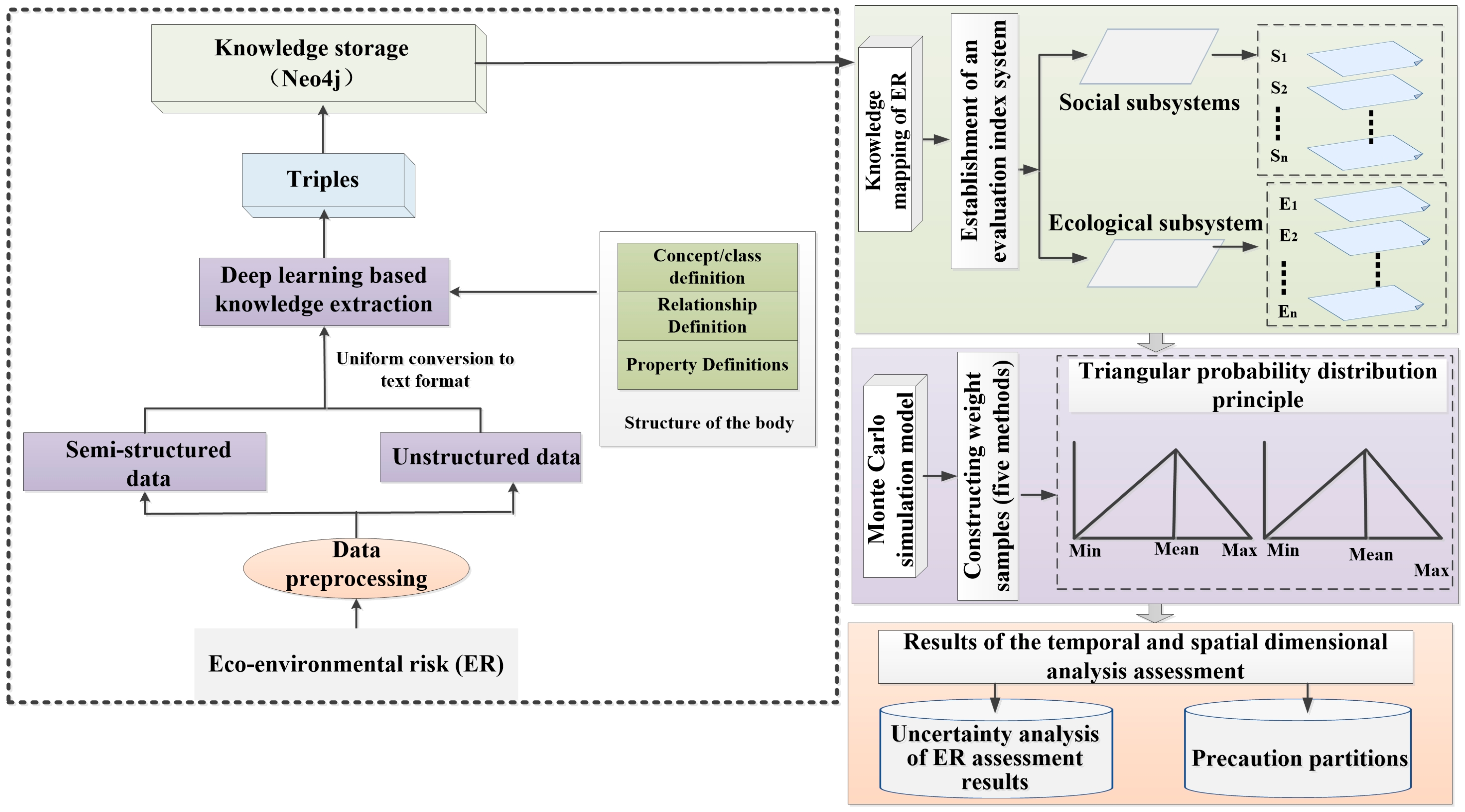
Figure 3.
Schema layer for the KG of ER.
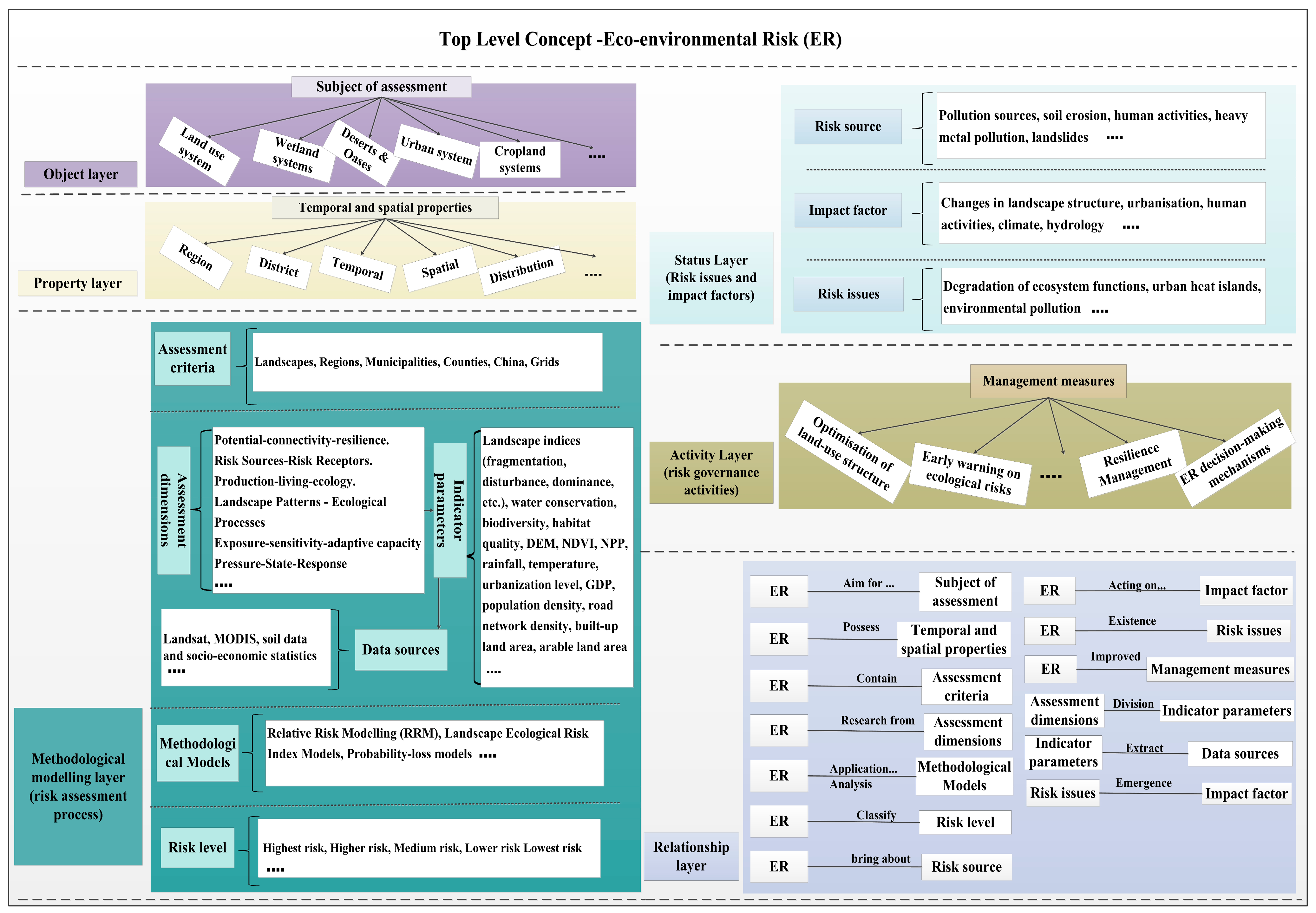
Figure 4.
Overall structure of the model.
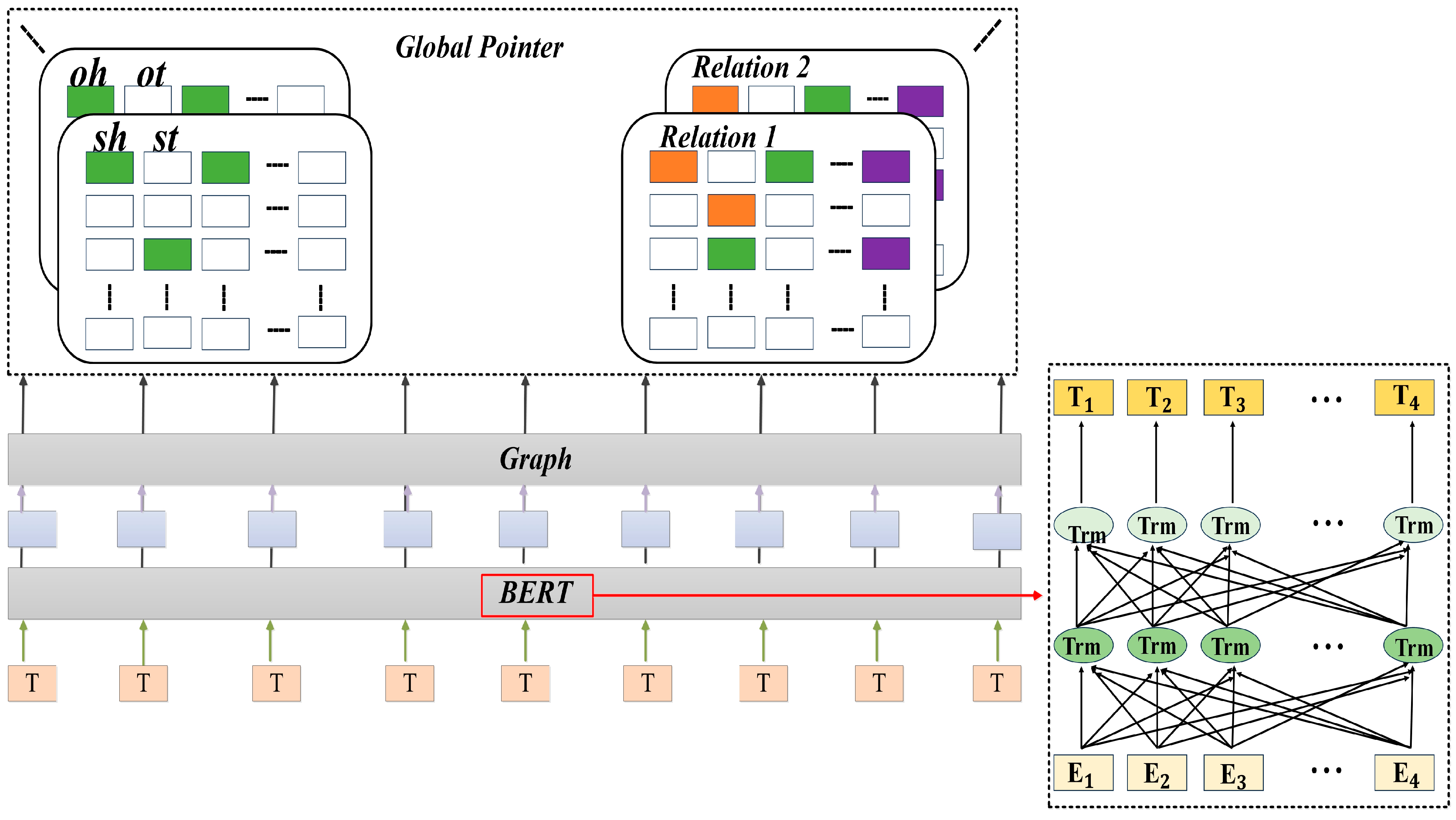
Figure 5.
The KG of ER based on Neo4j.

Figure 6.
Spatial patterns of ERs in the study area.

Figure 7.
Quantitative results of the subsystem (Contains: spatial patterns of social and ecological subsystem risk index; social and ecological subsystem risk index).
Figure 7.
Quantitative results of the subsystem (Contains: spatial patterns of social and ecological subsystem risk index; social and ecological subsystem risk index).
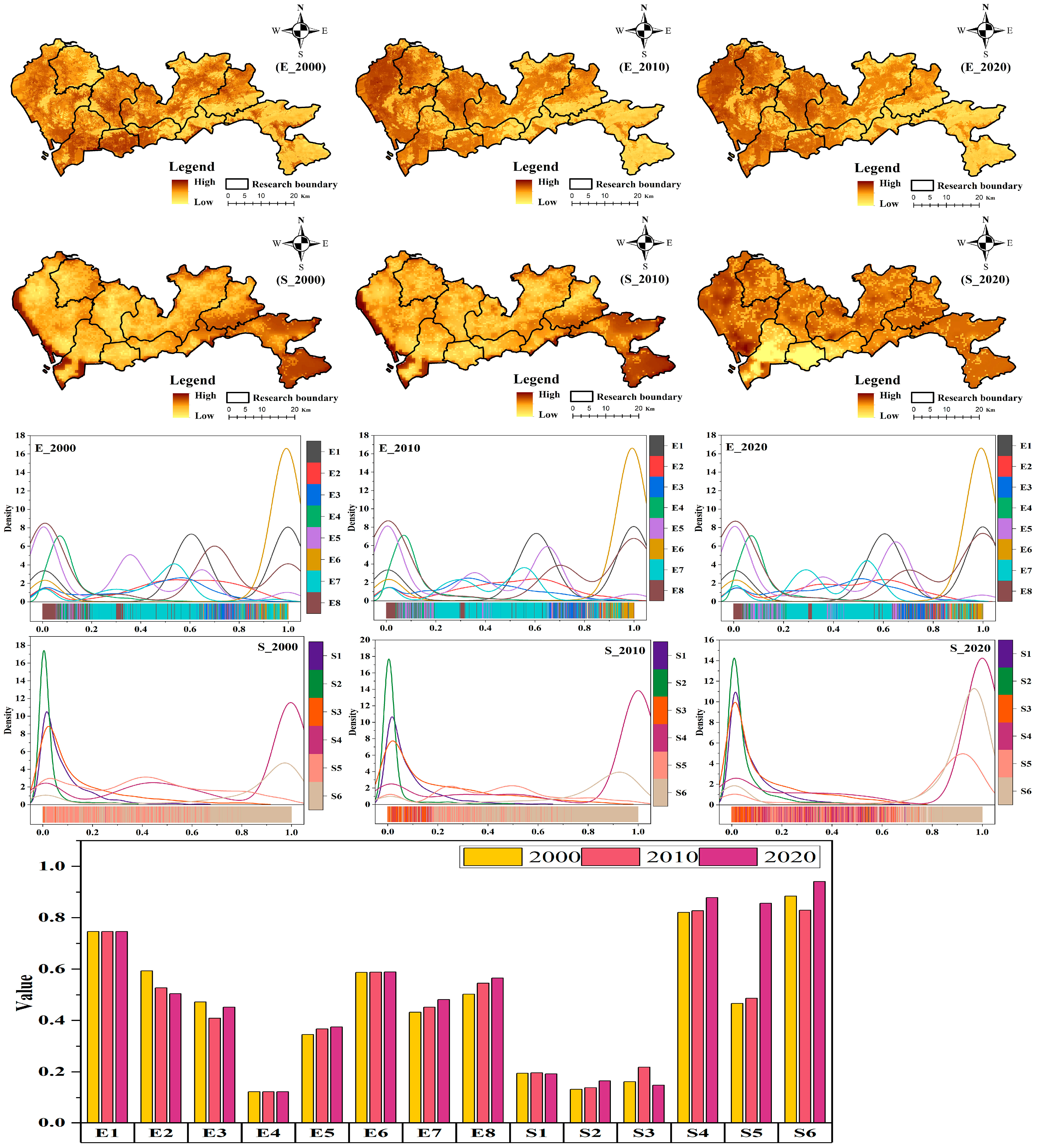
Figure 8.
Geographic location of sample points and uncertainty in the ER and its subsystems (2000).

Table 1.
Data categories and sources.
| Category | Data | Data Sources | Website Source |
|---|---|---|---|
| Spatial data | China Basin and River Network Dataset | Resource and Environmental Science Data Center of the Chinese Academy of Sciences | http://www.resdc.cn/ (accessed on 2 June 2023). |
| Vector boundary data | |||
| GDP Spatial Distribution Kilometer Grid Dataset (Resolution: 1 km) | |||
| Population Spatial Distribution Kilometer Grid Dataset (Resolution: 1 km) | |||
| Digital elevation data (Resolution: 30 m) | Geospatial data cloud | http://www.gscloud.cn/ (accessed on 3 May 2023). | |
| Land-use data (Resolution: 30 m) | |||
| Normalized Difference Vegetation Index (NDVI) (Resolution: 30 m) | |||
| Landsat remote sensing images | USGS website | http://glovis.usgs.gov (accessed on 14 March 2023). | |
| Chinese soil data set in the Harmonized World Soil Database (HWSD) | National Tibetan Plateau Data Center | http://data.tpdc.ac.cn (accessed on 1 February 2023). | |
| Point of interest data | Baidu Map Company, Beijing, China | http://map.baidu.com (accessed on 15 February 2023). | |
| Statistical data | Dataset of daily values of surface climate data in China (V3.0) | China Meteorological Data Network | http://data.cma.cn/ (accessed on 9 July 2023). |
| Food production | China Economic and Social Big Data Research Platform | http://www.data.cnki.net (accessed on 14 April 2023). | |
| Shenzhen Water Resources Bulletin | Shenzhen Municipal Government Portal | http://www.sz.gov.cn/ (accessed on 14 April 2023). | |
| Shenzhen Statistical Yearbook | China Yearbook Network | http://www.yearbook.cn/ (accessed on 15 April 2023). |
Table 2.
P, R, and F1 values of the model (Unit: %).
| Times | ) | ||
|---|---|---|---|
| Epoch = 50 | 0.82 | 0.81 | 0.81 |
| Epoch = 100 | 0.85 | 0.86 | 0.85 |
| Epoch = 200 | 0.86 | 0.86 | 0.87 |
Table 3.
ER Assessment Indicator System.
| Object | Subsystems | Indicators | No. | Indicator Character |
|---|---|---|---|---|
| ER | Ecological subsystem | Soil erodibility factors (K) | E1 | + |
| Surface temperature (LST) | E2 | + | ||
| Average annual rainfall | E3 | + | ||
| DEM | E4 | + | ||
| Carbon storage (Calculated by the InVSET model) | E5 | − | ||
| Soil conservation (Calculated by the InVSET model) | E6 | − | ||
| Water conservation (Calculated by the InVSET model) | E7 | − | ||
| Habitat quality (Calculated by the InVSET model) | E8 | − | ||
| Social subsystems | Population density | S1 | + | |
| Disturbance density of transport facilities | S2 | + | ||
| Industrial density | S3 | + | ||
| Food production per unit area | S4 | − | ||
| Economic density | S5 | − | ||
| Density of parkland | S6 | − |
Table 4.
The triangular probability distribution of each indicator weight.
| Indicator | Max | Min | Mean | Indicator | Max | Min | Mean |
|---|---|---|---|---|---|---|---|
| E1 | 0.064 | 0.015 | 0.037 | S1 | 0.101 | 0.009 | 0.052 |
| E2 | 0.102 | 0.023 | 0.062 | S2 | 0.089 | 0.049 | 0.068 |
| E3 | 0.095 | 0.014 | 0.063 | S3 | 0.088 | 0.012 | 0.054 |
| E4 | 0.084 | 0.015 | 0.055 | S4 | 0.115 | 0.018 | 0.071 |
| E5 | 0.106 | 0.019 | 0.064 | S5 | 0.533 | 0.035 | 0.168 |
| E6 | 0.131 | 0.017 | 0.072 | S6 | 0.135 | 0.021 | 0.078 |
| E7 | 0.156 | 0.014 | 0.074 | ||||
| E8 | 0.186 | 0.018 | 0.081 |
Table 5.
Area proportion of each level of ER.
| Year | Lowest-Risk Area | Lower-Risk Area | Medium-Risk Area | Higher-Risk Area | Highest-Risk Area |
|---|---|---|---|---|---|
| 2000 | 18.72% | 17.08% | 28.73% | 27.68% | 7.79% |
| 2010 | 20.27% | 17.88% | 21.07% | 26.79% | 13.99% |
| 2020 | 16.11% | 20.46% | 17.57% | 25.39% | 20.47% |
Table 6.
Moran’s I of the ERIs.
| Value | 2000 | 2010 | 2020 |
|---|---|---|---|
| Moran’ s I | 0.756 | 0.785 | 0.791 |
Disclaimer/Publisher’s Note: The statements, opinions and data contained in all publications are solely those of the individual author(s) and contributor(s) and not of MDPI and/or the editor(s). MDPI and/or the editor(s) disclaim responsibility for any injury to people or property resulting from any ideas, methods, instructions or products referred to in the content. |
© 2024 by the authors. Licensee MDPI, Basel, Switzerland. This article is an open access article distributed under the terms and conditions of the Creative Commons Attribution (CC BY) license (https://creativecommons.org/licenses/by/4.0/).
Share and Cite
MDPI and ACS Style
Yang, Y.; Zhu, X. Eco-Environmental Risk Assessment and Its Precaution Partitions Based on a Knowledge Graph: A Case Study of Shenzhen City, China. Sustainability 2024, 16, 909. https://doi.org/10.3390/su16020909
AMA Style
Yang Y, Zhu X. Eco-Environmental Risk Assessment and Its Precaution Partitions Based on a Knowledge Graph: A Case Study of Shenzhen City, China. Sustainability. 2024; 16(2):909. https://doi.org/10.3390/su16020909
Chicago/Turabian StyleYang, Yijia, and Xuexin Zhu. 2024. "Eco-Environmental Risk Assessment and Its Precaution Partitions Based on a Knowledge Graph: A Case Study of Shenzhen City, China" Sustainability 16, no. 2: 909. https://doi.org/10.3390/su16020909
Note that from the first issue of 2016, this journal uses article numbers instead of page numbers. See further details here.