Case Study on the Economic and Environmental Impact of the Introduction of the Variable-Rate Distribution of Fertilizer in Wheat (Triticum aestivum L.) Cultivation

Abstract

Fertilization plays a strategic role in the cultivation of wheat, contributing to harvest yield, both in quantitative and qualitative terms. However, similarly to all farm inputs, it has both economic and environmental impacts due to fertilizer dispersion into the environment during its distribution, as well as any excess fertilizer not used by the crop. Precision agriculture, which introduces the possibility of distributing fertilizer following prescription maps, has an immediate effect on dosage compliance according to the request and potential for use by each homogeneous area of the crop. An experimental field (about 15 hectares) at the Council for Agricultural Research and Economics (CREA) of Treviglio (BG) in Northern Italy was fertilized using a centrifugal fertilizer spreader combined with a tractor, equipped with a satellite system to distribute urea led by prescription maps. The purposes of this research were to verify (i) the effect of fertilization, performed with precision agriculture (PA) criteria at a variable rate; (ii) the comparison of the economic impact of the quantities of fertilizer required by precision agriculture compared to the distribution required in previous years (fertilizers administered according to conventional agriculture). The treated areas showed a significant yield improvement (almost 14%) when fertilization was performed according to the prescription map. With a negligible margin of error of less than 0.001, the total amount of fertilizer used was the same in both years.

1. Introduction

Fertilization is considered one of the key elements for achieving high yields in bread wheat (Triticum aestivum L.) cultivation. However, while fertilization inputs can be positive in the short term, they could seriously affect the sustainability of agricultural activity in the long run [1]. Nutrient deficiency can adversely affect plant health and growth and can decrease harvest yield. On the other hand, delivering excessive quantities of minerals to plants, exceeding their natural needs, is not only useless and expensive, but can also have negative effects on the environment, such as the pollution of groundwater and subsequently also of rivers and freshwater, creating unwanted imbalances [2].

Cultivated fields are rarely uniform; this is often due to the heterogeneous nature of the substrate. Crops show variability in all phases, from germination, to development, up to grain production [3]; therefore, the distribution of fertilization inputs for crops must consider actual variability, and especially variability in the proximity of input delivery time.

Current technologies make it possible to manage distribution with a site-specific approach through modulating mechanical parts of implements that increase or reduce the dosage according to the detected request [4]. These technologies can act through processing direct information obtained from sensors installed on the tractor acquiring data along the way (on-the-go), or they can release a distribution based on the indications entered in a previously elaborated prescription map. It is then possible to simulate this kind of procedure with a digital twin [5].

Currently, one of the methods for preparing prescription maps is based on indices calculated on spectral bands in the visible and near infrared (IR) wavelength range [6]. The spectral analysis is based on the behavior of reflective leaves as a function of the pigments that activate a photosystem, with maximum absorption at wavelengths of 700 nm and 680 nm [7].

Recent studies have shown high correlations between degree of coverage and biomass in the wavelength range of red, which has a wavelength of 678 nm with a correlation coefficient of r = 0.724, and in the near IR range, a wavelength between 721 and 1050 nm with r = 0.68 [3,8]. Ehlert and Dammer [9] have also shown a correlation between biomass and yield up to values of r = 0.56.

This leads to the hypothesis that the sensors, both proximal on-board tractors and remote sensors on satellites, comply with the requirements to accurately evaluate vegetation cover and facilitate early fertilization.

Mulla [10] stated that remote sensing plays an increasingly important role in near real-time management of soil, crops, and pests in precision agriculture (PA). The main purpose of using remote sensing data for PA is to identify the in-field variability of soil and plant properties. Remote sensing adoption optimizes crop management (i.e., crop yield would be maximized, also improving sustainability), as suggested by Ge et al. [11].

Spatial continuous data is critical in creating reliable prescription maps in precision fertilization. This data mainly refers to basic fertilization, where site-specific prescription zones form the basis of practical application based on discrete soil sampling [12].

Remote sensing data and methods have been successfully implemented in various applications in PA [13,14], and different statistical processing methods have also been adopted [15,16]. Several authors have also used open and commercial satellite data for real-time monitoring of agricultural crops [17,18,19,20,21]. Satellites allow high-frequency monitoring (with short intervals, e.g., less than 10 days) of agricultural crop conditions over large areas, regardless of the position of the observer [22,23]. Moreover, other authors [24,25] attribute great importance to the development of fully automated remote sensing methods with the aim of complete automation of satellite image processing.

Despite the fact that several approaches have been proposed to manage fertilization in PA, there is still not a recognized method for preparing prescription maps. The optimal choice of information source (i.e., proximal, remote, or on-the-go) and method to quantify the fertilizer to be applied is still under debate.

Therefore, this study, conducted over two years of wheat cultivation, aimed to: (i) compare fertilizer distribution applied with site-specific technologies (obtained with a traditional constant distribution), verifying the effect on crop yield, and (ii) maintain the same fertilizer (Nitrogen) amount per hectare, differentiating the dose in the second growing season, according to the clusters based on spectral information and from proximal sensors.

The information from the proximal and remote sensors were used both for the preparation of the prescription map, and for the monitoring of the crops after the two fertilization modes.

The information about the yield obtained at the end of the cycle is aimed to verify any difference in production according to distribution position. This way, it will be possible to define whether the input used in production has achieved any effect on crop yield.

2. Materials and Methods

The comparison test was performed in a field of 14.64 hectares, in the framework of experimental farming of the Council for Agricultural Research and Economics (CREA) of Treviglio (BG) in Northern Italy (45°30′50.86″ N, 9°32′36.15″ E). During the cultivation observation period, data on air temperatures and rainfall were collected at a weather station located within ~3 km of the experimental field [26]. In the two years preceding the test, the soil had been cultivated with alfalfa (Medicago sativa L.), cut, and harvested as hay five times per year⁻¹. The soil, representative of the area, consisted of an abundant skeleton and showed a humus content of 3%. The main physical-mechanical characteristics of the field were as the follows: sand = 68%; silt = 24%; and clay = 8%. In addition, the soil chemistry was characterized as follows: N availability of 118 kg ha⁻¹; P availability of 13 kg ha⁻¹; and K availability of 131 kg ha⁻¹. An expected mean output of 6 wheat tons ha⁻¹ requires an estimated amount of 180 kg ha⁻¹, 90 kg ha⁻¹, and 150 kg ha⁻¹ of N, P, and K, respectively. Given the soil profile, only N and P have been spread in sufficient percentages to make up the deficit. Only the remaining N requirement, totalling 150 kg ha⁻¹, was uniformly applied to the field in the first year. In the second year, constant background fertilization was repeated in the same amounts, while cover fertilization was done with three doses of N, with an average dose of 150 kg/ha, a lower dose of 20% less (120 kg ha⁻¹), and a higher dose of 20% more (180 kg ha⁻¹). The soil was plowed and arrowed before sowing. The sowing dates were 10 October 2018 and 13 October 2019, and the sowing density was 350 seeds m⁻² in both years.

The median humidity was 18% and the median resistance to penetration was 0.98 MPa, as evaluated by a penetrometer [27].

Before seeding of the wheat (Triticum aestivum L., Antigua variety), a winter-spring crop, the soil was plowed, followed by harrowing for the seedbed preparation. The test was performed in the two-year period 2018–2020, comparing two seasons of wheat (Triticum aestivum L., Antigua variety) production. Fertilization with urea, before the stem elongation stage, was carried out with a centrifugal spreader (Sulky Dx30+, Sulky-Burel, Chateau Bourg, France) with a working width of 24 m, operating in two independent sections thanks to two discs moved by electric engines. The spreader was transported by a tractor equipped with a satellite system (StarFire6000).

In the two years covered by this study, fertilization, using the same average dose (150 kg) per hectare (150 kg ha⁻¹), was performed according to two different criteria. In 2019, the amount was distributed evenly over the field, without any distinction between clustered areas. An attempt was thus made to exploit the advantages of precision agriculture, considering the ability of the fertilizer spreader machine to evenly distribute the dose and contain overlapping. In 2020, the fertilization method involved the distribution of the same fertilizer (Urea 46% N), differentiating the dose according to the clusters prepared based on spectral information from Sentinel 2 satellite and from proximal sensors mounted on the tractor, ten days before fertilization, during the rolling operation. Figure A1 shows the flow chart that differentiates the test conducted in 2019 and 2020.

2.1. Remote Information

The satellite (Sentinel 2 maps were obtained from the reflection bands of the available spectra, available at the ESA (European Space Agency–Explore data|Copernicus Data Space Ecosystem) website [28].

The data obtained, ortho-corrected by ESA [28], belonged to the so-called Level 2A category, with atmospheric correction (without cirrus band B10). The data were imported and processed through R software, using the sen2r function of the “sen2r” package, where both satellites 2A and 2B were set as sources. Level 2A processing included scene classification and atmospheric correction applied to Top-Of-Atmosphere (TOA) level 1C orthoimage products.

The main level 2A output was a low atmosphere-corrected reflectance orthoimage product. The resolution of the bands required was 10 × 10 m.

From the bands obtained, the three classic RGB bands [(blue (σ = ~493 nm), green (σ = ~560 nm) and red (σ = ~665 nm)] and a NIR (Near Infra-Red) (σ = ~833 nm) were calculated for each pixel of the maps, as suggested by Bremer et al. [29]. The spectral indices NDVI (Normalized Difference Vegetation Index) was defined by the formula:

NDVI = (NIR − Red)/(NIR + Red)

(1)

As suggested by Nigon et al. [30], the MCARI2 (Modified Chlorophyll Absorption in Reflectance Index 2) was defined by the formula:

MCARI2 = {1.5 [2.5(ρ800 − ρ670) − 1.3(ρ800 − ρ550)]}/√ [(2ρ800 + 1)² − (6ρ800 − 5√ ρ670) − 5]

(2)

These formulas have been chosen from the indices studied for their high capacity to detect the homogeneity of the photosynthetic activity of crops [31,32]. In particular, the NDVI was chosen for the wealth of information it provides and its validation history, and the MCARI2 index was chosen because it is considered one of the best predictors of the green leaf area index [33,34,35].

The MCARI2 index incorporates an adaptation factor in soil, preserving sensitivity to the leaf area and resistance to the influence of chlorophyll. From the composition of the visible spectrum bands, those relating to red (R), green (G), and blue (B), the images collected were checked and were processed only if there was no cloud formation over the field.

2.2. Proximal Information (Proximal Sensors on Board)

The proximal sensor system consisted of two RGB optical matrix imaging sensors (left and right) and the related algorithm, called Canopyct [36]. The Canopyct output is called the Canopy Index (CI), a pure number ranging from 0 to 1000. The Canopyct algorithm is based on analysis of the images provided by the two RGB imaging sensors. For each of the two imaging sensors, after calculating the hue (H), saturation (S), and brightness (L) coordinates of each pixel of the image from its R, G, and B components, Canopyct calculated a linear combination of R, G, and B coordinates and the H, S, and L of each pixel in order to compress the data into a single dimension and maximize the meaning of the data set. Then, a thematic map was obtained from the instantaneous image collected by the RGB sensor via the application of a grouping technique to the entire image, which assigned each pixel to the vegetation using a statistical data processing algorithm based on a “two-class” implementation of the Jenks Natural Breaks classification method [37]. Finally, the CI was calculated using the formula below:

CI = (Npixvegetation/Npixtotal) × 100

(3)

where:

Npixvegetation = total number of pixels in the image that have been classified as “vegetation”

Npixtotal = total number of pixels in the image

The total CI for a single position was derived from the average of the left and right sensor contributions. Different levels of intelligent data filtering techniques were applied to the collected data to remove left or right readings that were unrelated to the culture. The Canopyct algorithm is insensitive to changes in light and lighting conditions as it is intrinsically able to compensate for these differences, and it is also impartial towards the variations that can occasionally occur in the exposure settings of the matrix-based RGB optical imaging sensors upon which the readings are based.

2.3. Data Analysis for the Prescription Maps

The methodology for preparing the prescription maps consisted of a first phase of cleaning the data with a “boundary advance” of five meters with respect to the edges in order to reduce the possible effect of the roads and hedges that surround the field. This measure was applied to data from both satellite and proximal sensors. In the second phase, only the values of the sampling coordinates of the proximal sensors were extracted from the satellite maps. In this way, the prepared dataset for the same coordinates consisted of the values of the two spectral indices sought (NDVI and MCARI2) and the values provided by the proximal sensors. Subsequently, a multivariate analysis of the principal components (PCA) was performed on the dataset to verify how these factors contributed to the distribution of the coordinates.

A k-means analysis was performed on the same dataset, searching for the most appropriate clustering value, which was then used as a criterion for determining the areas of different nutritional management. A k-means clustering was performed using the pam function of the cluster package of the R software. The PAM function is a more robust version of k-means [38,39], used to compare different combinations of clustering based on the lowest value of the average silhouette width.

2.4. Production Information (Geolocated Harvester) and Statistical Analysis

The yield distribution maps were obtained by harvesting using a geolocated combine harvester (John Deere S770) with a cutting width of 13.70 m, equipped with an automated driving system (Autotrac^TM) which allowed path optimization via the avoidance of overlaps, thus ensuring that the working width was fully exploited as much as possible. The measurement of the harvested quantity took place using a volumetric system in the auger that carried the grain to the bin.

Yield calibration occurred in real time using a system of three sensors positioned inside the bin (ActiveYield^TM), which were also able to evaluate grain moisture variations.

The geolocation was obtained through a satellite position detection system with RTK (Real Time Kinematics) digital correction. In addition, as indicated by Cordoba et al. [40], outliers were treated to avoid errors generated by the cutter bar of the harvester. The study provided the comparison of yield at the same fertilization rate, i.e., 150 kg of N ha⁻¹, in both years. 388 points were obtained from field coordinates.

The raw yield data underwent processing with a (i) Shapiro–Wilk test for normal distributions, (ii) Levene’s test for equal variances, (iii) ANOVA based on yield year⁻¹ and dose, and (iv) Tukey’s test, applied for post-hoc analysis in order to identify the effectiveness of the treatments.

3. Results

Meteorological data showed similar trends between the two years compared. In 2018–2019, the average temperature was between a minimum of −1.12°C in January and a maximum of 27.56 °C, while in 2020 the average temperature was between a minimum of 0.13 °C in January and a maximum of 27.56 °C. Monthly rainfall in 2018–2019 reached a maximum of 219.3 mm in the month of June, with overall rainfall of 838 mm, and in 2019–2020 maximum monthly rainfall of 240.3 mm was observed again in the month of June, with overall rainfall of 1058.7 mm. The temperature values and rainfall for the studied years are shown in Figure A2. 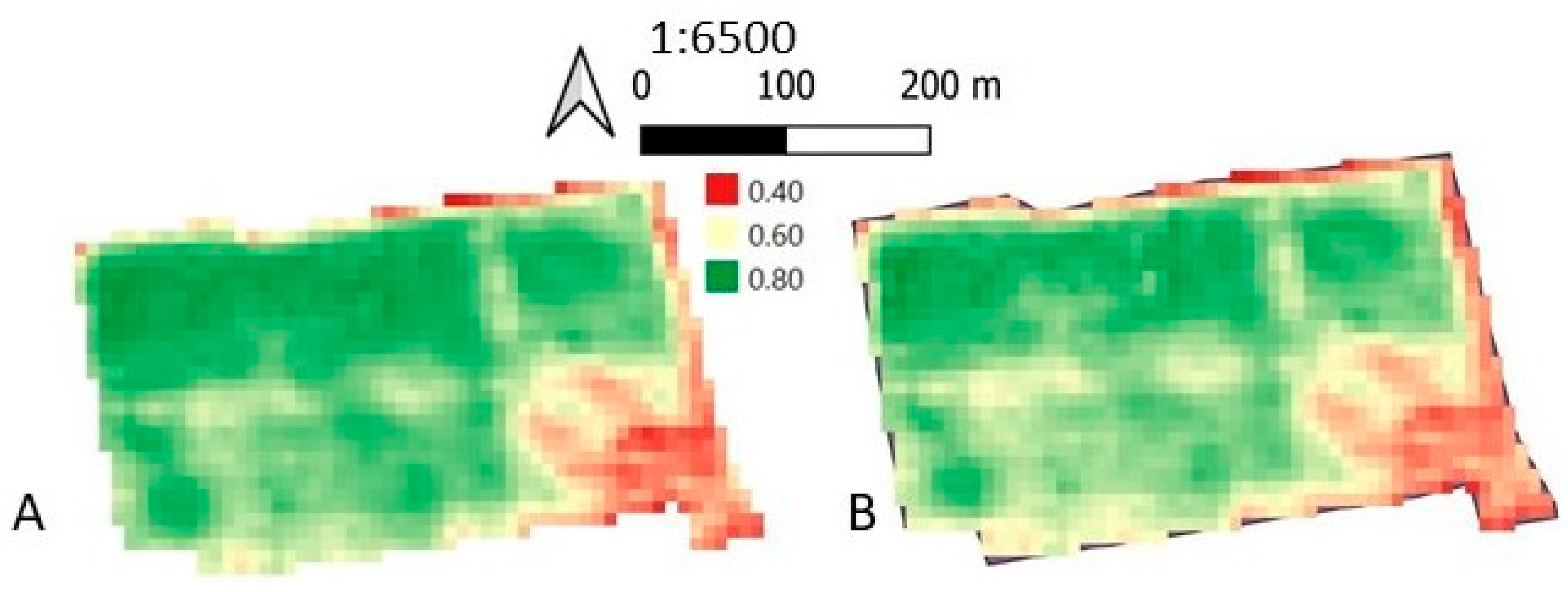In the first year of testing, fertilizer was distributed by setting the fertilizer spreader with a constant value of 150 kg of N ha⁻¹. The distribution map was developed according to the request, with an average distribution error of 0.67%, with a total consumption of 2206 kg of fertilizer. The map of the NDVI index distribution obtained from the satellite spectral bands on 15 March 2019 is shown in Figure A3. The distribution had an average NDVI value of 0.594, with a range of 0.278–0.654 and standard deviation of 0.134.

The yield map, after the treatment of the outliers, is shown in Figure A4. This map shows an average yield value of 3.15 t ha⁻¹, with a minimum of 0.8 t ha⁻¹, a maximum of 5.83 t ha⁻¹, and a standard deviation of 0.57 t ha⁻¹, with a total weight of 54.78 t of grain collected. The distribution of variability in physical soil analysis was integrated into the yield map. It can be observed that clay, silt, and sand components are variable in the identified areas.

This framework affects overall crop inequality. Fertilization, more than other agricultural practices, must match this variability.

In the second year of testing, fertilization was performed based on the prescription map built by integrating satellite NDVI information (17 March 2020) with information obtained from the proximal sensors used during the rolling operations at the end of the tillering phase (13 March 2020).

The average fertilizer dose (150 kg of N ha⁻¹) was equal to that of the previous year, but the distribution took place on the basis of a prescription map with three identified clusters.

The cluster identification process considered the distribution map of the NDVI index obtained by satellite, six days prior to the distribution of the fertilizer, and the map of the canopy index obtained with the proximal sensors, seven days before the distribution of the fertilizer. The proximal sensors were placed on the roof of the tractor during the rolling of the wheat, shortly before the stem elongation stage.

The satellite map of the spectral bands obtained on 17 March 2020, six days before the spreading date of the fertilizer, showed an average crop NDVI of 0.682, with a range of 0.381–0.818 and standard deviation of 0.092. Figure A5 shows the false color map of the distribution of NDVI and MCARI2 values.

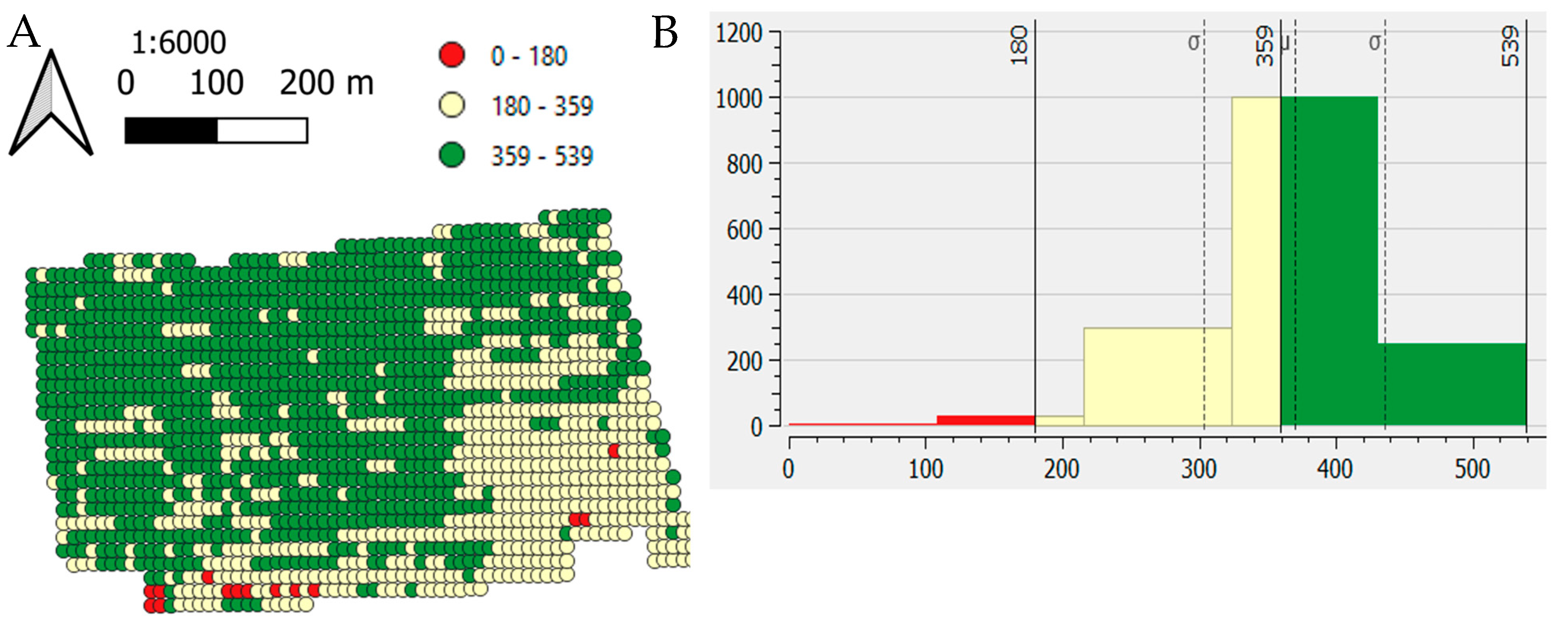
The map of the vegetative vigor values on 16 March 2020, seven days before the distribution of the fertilizer to the crops, showed an average vigor value of 359.33, with a range of 110–539 and standard deviation of 89.83. Figure A6 shows the distribution map (A) with false color of the vegetative vigor values (B).

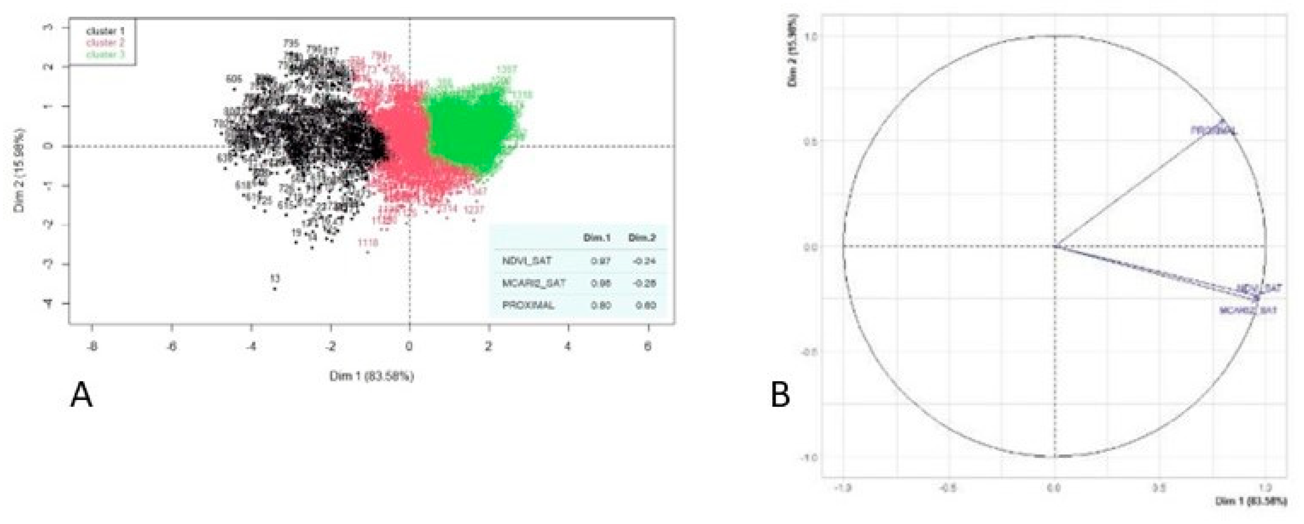
Principal component analysis (PCA) was developed using the PCA function of the FactoMineR package of the R software (version R 4.2.3) [41].

Elaboration showed that the cloud of points representing the sampling coordinates was distributed according to the vectors of the spectral indices NDVI and MCARI2 and the values of the proximal sensor. In the biplot shown in Figure A7, the coordinates with larger values as related to the three observed factors (Figure A7A) are placed in the right part of the graph, while the points representing decreasing values are in the left side of the graph.

The k-means analysis suggested clustering in two (average silhouette width = 0.52) or three (average silhouette width = 0.40) clusters. The three cluster option was chosen and thus informed the possibility of treating the three corresponding cluster areas with three different doses of fertilizer. To this end, each cluster was fertilized with a different dose of N ha⁻¹ (i.e., 120, 150, and 180 kg N ha⁻¹).

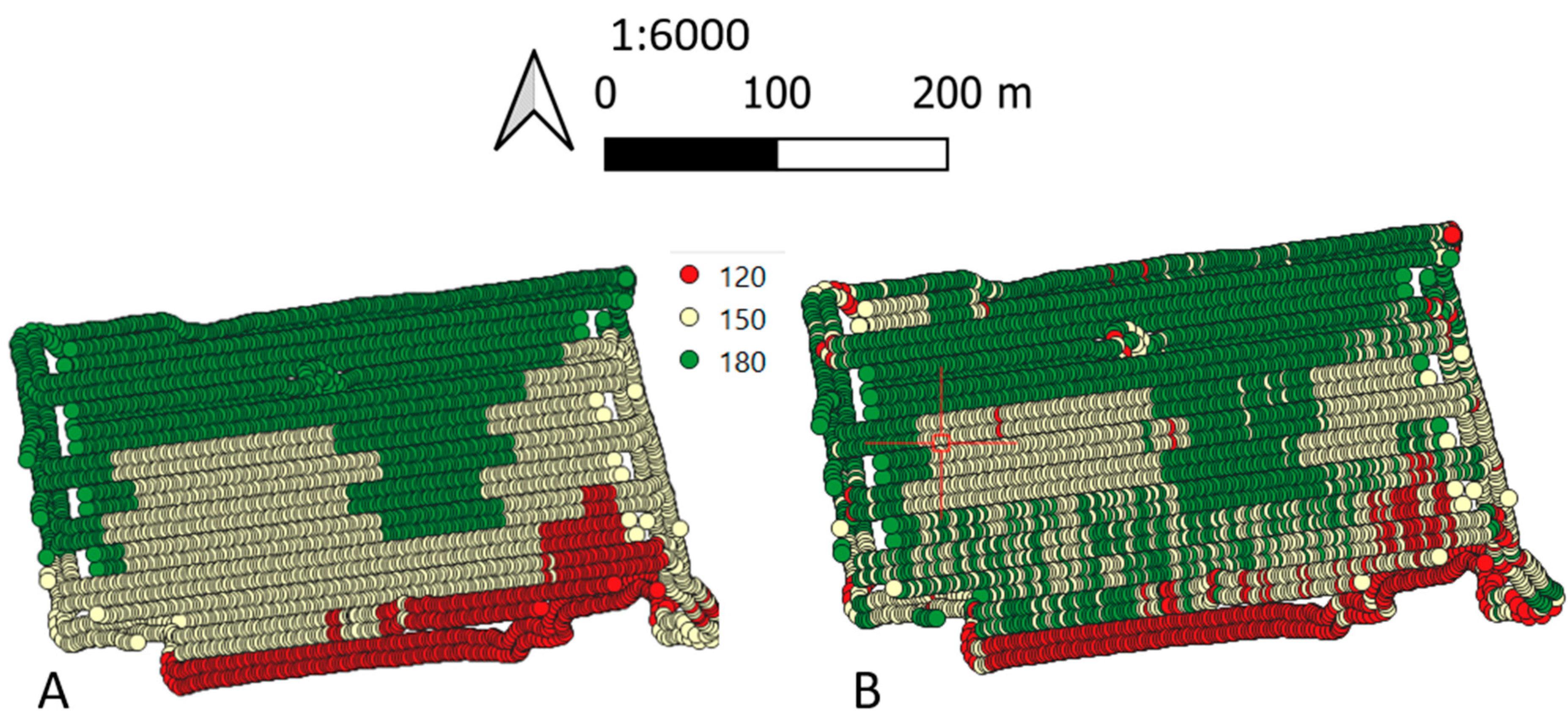
The prescription map (based on the k-means clustering) is shown in Figure A8 on the left (A). Moreover, after a smoothing and adaptation operation of the fertilizer spreader management software, the profile on the right (B) was developed, corresponding to the distribution performed map, with an average distribution error equal to 2.99% and a total consumption of 2206 kg of fertilizer.

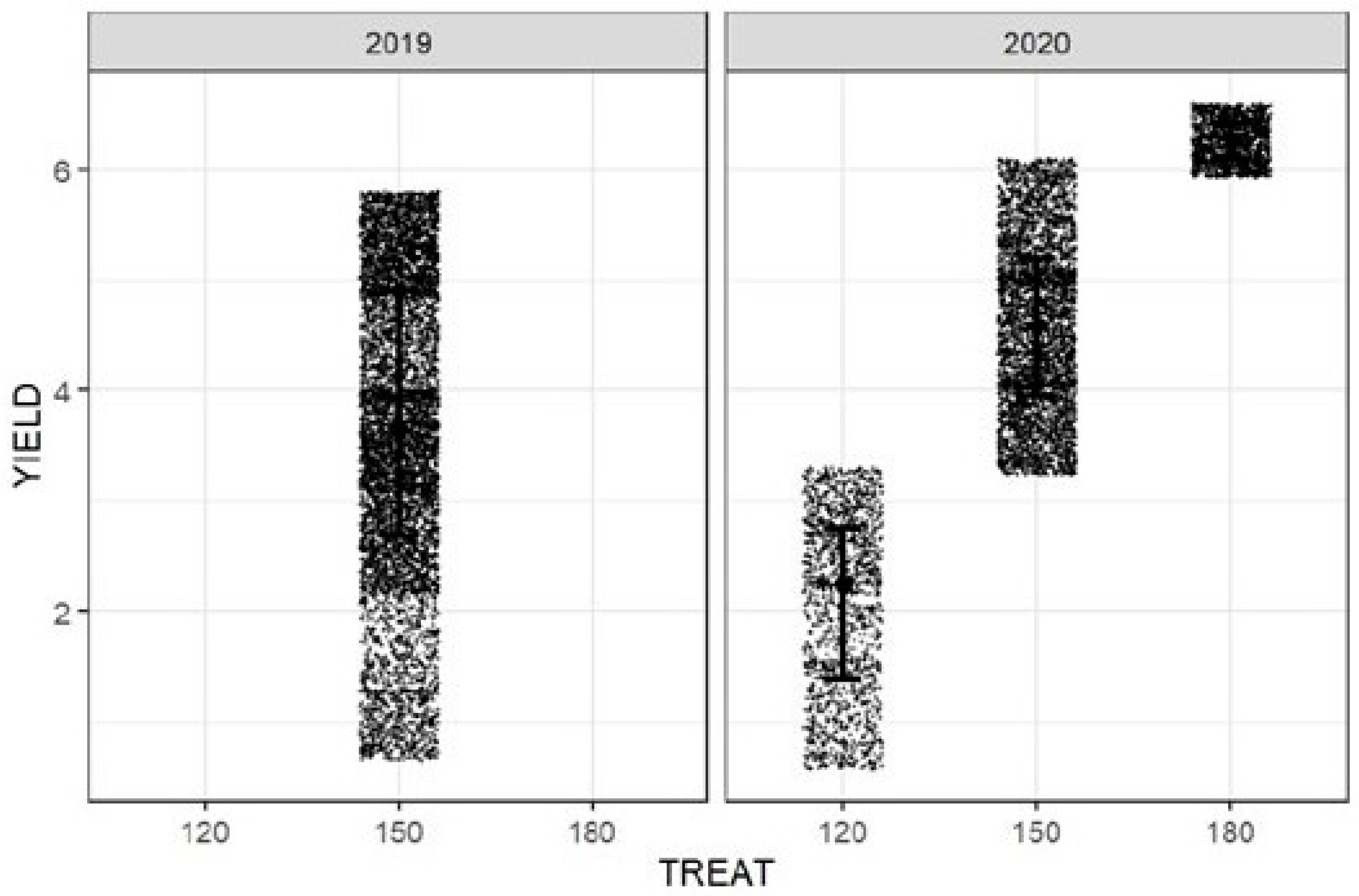
Two rectangular-shaped sub-plots (60 m × 130 m and 40 m × 70 m), depicted in Figure A9, were fertilized based on the same fertilizer rate, i.e., 150 kg of N ha⁻¹ in each of the two studied years. The distribution of yield values recorded at their coordinates in 2019 and 2020 has been studied.

The NDVI and MCARI2 index distribution obtained from the satellite spectral bands on 27 March 2020, which are reported in

Table 1. Average NDVI and MCARI2, from satellite maps, pre- and post-fertilization.

	2019		2020
Indexes	μ ± σ	Date	μ ± σ	Date
NDVI pre	-	-	0.682 ± 0.092	17/03
NDVI post	0.594 ± 0.134	15/03	0.781 ± 0.061	27/03
MCARI2 pre	-	-	0.432 ± 0.237	17/03
MCARI2 post	0.475 ± 0.284	15/03	0.653 ± 0.138	27/03

, show an average NDVI value of 0.781, with a range of 0.653–0.789 and standard deviation of 0.061, and an average MCARI2 value of 0.653, with a range of 0.367–0.687 and a standard deviation of 0.138. Increases were observed compared to the reading before fertilization and were even greater than the values recorded in the previous year.

The wheat harvest in 2020 took place on June 29. Figure A10 shows the distribution of the dry yield values in tons ha⁻¹. The average of the yield values was 3.99 t ha⁻¹, with a minimum of 1.32 t ha⁻¹, a maximum of 6.67 t ha⁻¹, and a standard deviation of 0.43 t ha⁻¹. A total weight of 59.24 t of grain was collected.

Table 2. Average yields (μ) with the respective standard deviations (σ) and the total productions obtained in the two years of the trial, distributed by yield classes. The weighted averages (μp) were calculated based on the respective surfaces. Different letters represent different groups based on the Tukey’s test.

	2019		2020
Yield Class	μ ± σ	Yield (t)	μ ± σ	Yield (t)	Treatment 2020
5.90–6.70	- -	- -	6.27 ± 0.29 a	19.31	180
5.00–5.80	5.43 ± 0.28 a	20.68	5.32 ± 0.25 b	14.26	150
4.10–4.90	4.51 ± 0.28 b	9.95	4.41 ± 0.30 c	14.11	150
3.20–4.00	3.61 ± 0.44 c	13.39	3.57 ± 0.37 d	9.07	150
2.30–3.10	2.75 ± 0.27 cd	7.32	2.62 ± 0.30 de	3.98	120
1.40–2.20	1.82 ± 0.27 d	1.96	1.79 ± 0.25 f	1.13	120
0.50–1.30	0.98 ± 0.19 e	0.97	0.82 ± 0.29 g	0.81	120
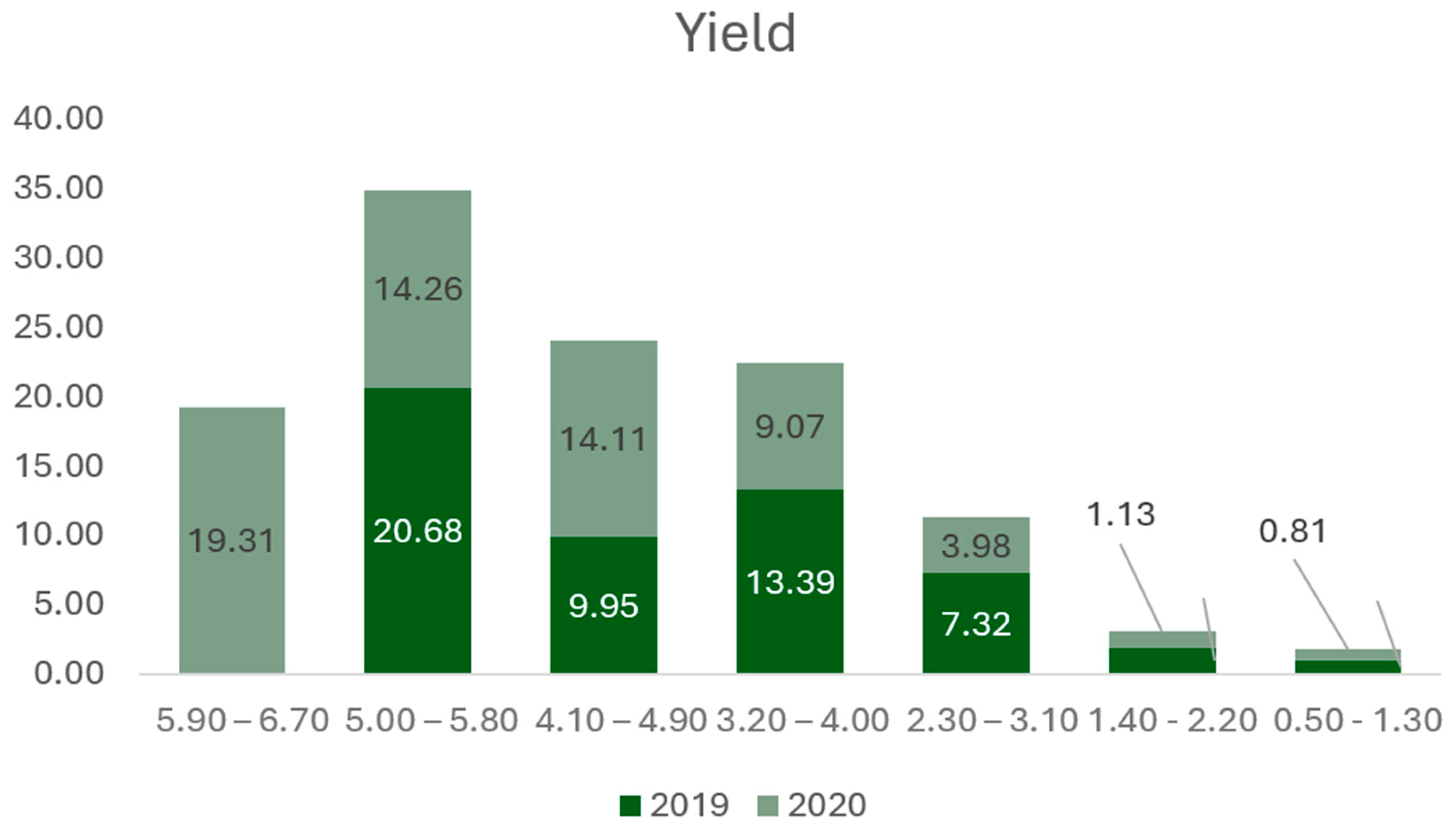
	μp = 3.71 ± 1.38	Σ = 54.27	μp = 4.55 ± 1.59	Σ = 61.86

shows the results of the yields obtained in the two years observed, distributed by yield clusters, with an indication of the fertilization treatment performed in 2020. The weighted averages of the yields obtained in the two trial years, calculated on the average yield of each class for the surface from which it was obtained, showed the difference in average yield recorded in the year 2020, in which fertilization was administered based on prescription maps.

It can be noted that the highest yield class, between 5.90 and 6.70, is absent in 2019. Overall, in 2020, 7.59 t more of caryopsis was collected than what was collected in 2019. The distribution of data, viewable in Figure A11, shows that in 2020 some classes, specifically the minor ones, responded with a lower production, having received reduced fertilizing treatment compared to the previous year. The majority of the points that received treatment with 180 kg ha⁻¹ of fertilizer exhibited a consequent increase in the yield produced at those points. In this way, a new production class (5.90–6.70) was created, represented by the points that previously belonged to the lower classes.

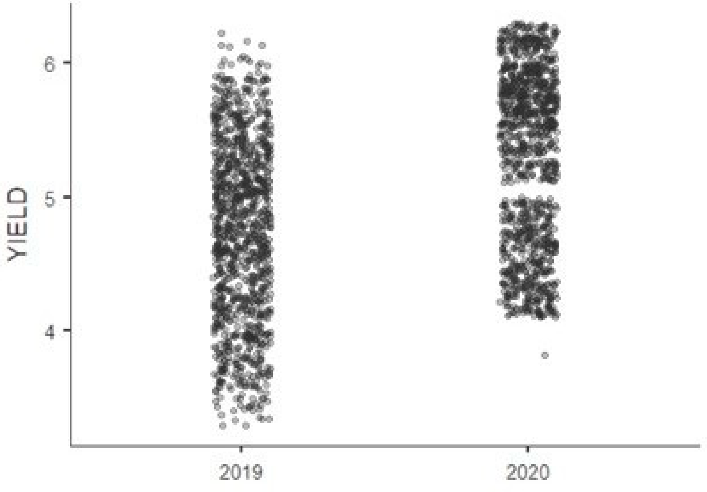
The coordinates handled with the same 150 kg of N ha⁻¹ dose in both years produced an average of 4.74 ± 0.663 in 2019 and 5.29 ± 0.645 in 2020 respectively (all measurements in tons ha⁻¹). The mean difference is not statistically significant (p-value > 0.05), showing that the conduction year did not affect the results (Figure A12).

Crop production, which increased overall, decreased slightly in the lower classes, which received a reduction in treatment (from 150 to 120 kg ha⁻¹). The areas fertilized using the same treatment of 150 kg ha⁻¹ did not undergo significant changes in production, but the areas fertilized using the increased treatment amount (180 kg ha⁻¹) in the year 2020 achieved a new production class (5.90–6.70). This is evident in the productions histogram shown in Figure A13, where it can be observed that the classes 3.20–4.00 and 4.10–4.90, which received the same treatment size across the two years, reduced their production in 2020, probably because they were counted in the highest class.

4. Discussion

The transition from the constant distribution mode of a fertilizer spreader to the variable rate mode, led by a prescription map, represents a fundamental step in the application of precision agriculture criteria [42]. Thanks to this study, the two types of distribution were compared using a centrifugal fertilizer spreader whose dose was controlled by a control unit with ISOBUS communication. Therefore, it was possible to guarantee both the uniformity of the distribution in all of the test field coordinates, and to guarantee the corresponding dose according to the prescription map provided before fertilization, based on the spectral indices from Sentinel satellite (sensu lato), as indicated by Santaga et al. [43], following the information ensured by proximal sensors.

The results showed that the experimental variable distribution increased the yield by almost 12%, in agreement with other studies [44,45]. These authors stated that the variable fertilization was applied according to data recorded from multispectral cameras proximal to the crops. The results of this study are also consistent with those obtained by Vizzari et al. [46].

Past study authors have not observed a decrease in grain yield under reduced N ha⁻¹ administration when using variable fertilization approaches. In the present experimental trial, an increase in yield was achieved in areas where the highest dose of fertilizer was administered, as could be expected. It is noteworthy to state that the areas that were treated with lower doses of fertilizer did not exhibit a corresponding reduction in yield. Thus, the whole field overall had a larger yield. However, as highlighted by several studies [47,48,49], the advantages of variable fertilization are not only related to an increase in yield. In fact, variable distribution, in which fertilizer doses are matched to cultivation needs point by point, is tailored to recognize fertilizer amounts that may not be assimilated by crops, leading to a consequent reduction in the risk relating to the impact of excess fertilizers on aquifers [50].

Furthermore, Katyal et al. [51] argued that variable distribution can also be improved by incorporating information relating to soil moisture into the process. The meteorological trend recorded across the two test years was consistent, with characteristic low rainfall values common across the two years. However, the real effects of variable fertilization should be observed over a longer period; they may be influenced by longer term climatic trends, as indicated in a similar study [46]. Therefore, the trial will continue for a long-term validation period, and using other crop species (e.g., Zea mays L., Hordeum vulgare L.).

This experimental activity is a “touchstone” in the data collection, and it is also a pilot study.

The results also provide an innovative contribution to the development of environmental policies aimed to reduce both production input (e.g., agrochemicals and fossil fuels) and the environmental impacts of cropping systems. An information management system can be proposed at farm level, with adequate training obtainable at no additional cost given that Sentinel 2 satellite maps are freely available.

5. Conclusions

The main objective of the experimental activity reported in this article was to verify the productive response of a winter herbaceous crop (Triticum aestivum L.), commonly cultivated in the area examined in this trial (the overall Po Valley). The test was carried out following a fertilization performed on the same field across two subsequent years: a uniform fertilization the first year, and a site-specific fertilization the second year. Although different fertilization doses were used between the first and the second year, double observation reduced the effect of environmental variability, which provided improved sturdiness in the data analysis. The prescription map, which guided the distribution of three different doses of nitrogen fertilizer, was set based on clusters characterized using information about the distribution of the NDVI spectral index, which was confirmed by the Sentinel 2 satellite and based on the force map obtained from proximal sensors.

The distribution of the yield obtained in the field showed that the areas treated with a reduced dose of fertilizer in year two exhibited lower production, but there was still an overall increase in yield. In particular, the concentration of treatment in some areas significantly improved production, which contributed greatly to the overall yield increase.

The overall quantity of fertilizer used, which was monitored in both years, measured the weight variation of the hopper during distribution and allowed verification of a desirable level of fertilization.

Furthermore, the study monitored the constant condition of 150 kg ha⁻¹ of fertilizer and compared the prescription map with three areas under different management (120, 150, and 180 kg ha⁻¹). The total amount of overall fertilizer over the two years was the same, with a negligible error of less than 0.001.

This study aimed to verify the possibility of a practical application of precision agriculture, showing results achievable with accessible tools, such as the distribution of the spectral index NDVI values. Although these data are freely available if obtained by satellite, a future test could compare them with the same indices obtained by drones. In fact, drones will ensure a better robustness of data.

The experimental activity will continue with the same application in other fields, and in the same field with a spring-summer crop, to verify the response of another crop (e.g., corn or sorghum) in another season of the year.