Low-Pressure Steam Generation with Concentrating Solar Energy and Different Heat Upgrade Technologies: Potential in the European Industry

Abstract

The industry is currently responsible for around 21% of the total CO₂ emissions, mainly due to heat production with fossil fuel burners. There are already different technologies on the market that can potentially reduce CO₂ emissions. Nevertheless, the first step for their introduction is to analyze their potential on a global scale by detecting in which countries each of them is more attractive, given their energy prices and resources. The present work involves a techno-economic analysis of different alternatives to replace industrial gas boilers for low-pressure steam production at 120 °C and 150 °C. Solar Heat for Industrial Processes (SHIP) was compared with Electric Boilers (EBs), High-Temperature Heat Pumps (HTHPs), and Absorption Heat Transformers (AHTs). SHIP systems have the potential to reach payback periods in the range of 4 to 5 years in countries with Direct Normal Irradiance (DNI) values above 1400 kWh/m²/year, which is reached in Spain, Italy, Greece, Portugal, and Romania. HTHPs and AHTs lead to the lowest payback periods, Levelized Cost of Heat (LCOH), and highest CO₂ emission savings. For both AHTs and HTHPs, payback periods of below 1.5 years can be reached, particularly in countries with electricity-to-gas price ratios below 2.0.

1. Introduction

The European industry is currently responsible for 21% of total CO₂ emissions [1]. Tackling this sector is hereby a key point to make Europe carbon-neutral and resource-efficient by 2050, as targeted in the European Green Deal [2,3]. Around 66% of industrial energy use is for process heat, and approximately 77% of the energy comes from non-renewable energy sources. Industries often require steam at temperatures from 100 °C to 200 °C. This temperature range involves 26% of the total process heat demand, and the heat is generally produced with fossil fuel burners. According to Dengler et al. [4], 70% of the boilers are gas-fired in Europe. Practically half of the industrial heat generated from non-renewable energy sources comes from natural gas [1].

According to Fox et al. [5], in the USA, several sectors, such as the pulp and paper or chemical industries, are among the top steam consumers, similar to the situation in European industry [6]. In the USA, out of the total fuel consumption, steam generation accounts for 89% of the pulp and paper industry and 60% in the chemical sector [7].

Different alternative technologies are under study [8] to reduce the CO₂ emissions derived from industrial heat requirements, such as biomass, solar thermal, or geothermal energy. According to Kempener and Saygin [9], by 2030, a third of the industrial heat demand could be potentially achieved with 13% solar thermal, 13% biomass, and 7% geothermal heat pumps. Whenever waste heat is available, heat recovery and upgrades using high-temperature heat pumps (HTHPs) or Heat Transformers are also efficient options to reduce CO₂ emissions. The introduction of any of these alternatives can play a key role in sustainability, but requires a cross-disciplinary approach considering economic, technical, and environmental issues. The main objective of the present work is to compare potential alternative technologies to produce low-pressure steam for industry at temperatures of around 120 °C (2 bara) and 150 °C (4.7 bara).

Regarding the application of HTHPs, Kosmadakis et al. [10] highlighted Finland, Sweden, and Switzerland as particularly promising European countries due to their low electricity-to-gas price ratio. In such countries, payback periods of 3 years or shorter can be potentially achieved. HTHP technologies and applications are being explored within the recent IEA HPT Annex 58 [11]. Among the market barriers to increasing the industrial heat pump uptake are a missing awareness and experience [12] for end-consumers, installers, and engineers [13,14,15]. The demanding integration of tailor-made systems [16], with no plug-and-play solutions, is also considered among the main drawbacks of HTHPs.

Solar thermal energy is another potential technology for industry to produce steam since the temperatures reached are very wide, ranging from 50 to 400 °C or more, by concentrating the beam radiation [17]. Solar Heat for Industrial Processes (SHIP) is currently in the early stages of development and has, among others, been explored within the IEA SHC Task 49 [18] or in the IEA Task 64 on solar process heat [19]. The most common technologies in SHIP systems are either parabolic trough collectors or Linear Fresnel (LFR) collectors [20]. However, despite their techno-economic potential in industry, actual deployment levels remain relatively low [21]. Weiss and Spörk-Dür [22] reported that in 2021, there were at least 975 SHIP systems in operation worldwide. According to the International Renewable Energy Agency, shorter payback periods should be achieved for a higher market penetration. Still, this barrier may be reached in the short term given the inflation on gas in the period 2021–2023.

Although there are already different technologies available to reduce the carbon footprint of industry [23], it is often unclear which measures are most economical [24]. Furthermore, given the high differences between countries concerning the energy price, and the indirect CO₂ emissions of their electric power production, it is important to know the potential of each technology given the characteristics of each country. In SHIP systems, the energy source, which is the Direct Normal Irradiation, also has a key impact on economic feasibility. All of these variables should be considered by energy planners to determine the potential integration in the industry.

Most of the available techno-economic assessments have been devoted to one specific technology, such as HTHPs alone or solar thermal systems alone. For example, Kosmadakis et al. [10] simulated different HTHP systems for their potential application in European industry. Zhao et al. [23] compared different HTHP systems, especially focusing on the Coefficient of Performance (COP) and the total cost. De Santos López [25] simulated SHIP installations for industry. Vieren et al. [26] calculated the techno-economic performance of industrial HTHPs using a simple cycle configuration and a discount method for the economic analysis. Filali Baba [27] recently conducted different case studies to compare the techno-economic performance of different fossil fuel boilers with LFR collectors.

In some specific cases, two technologies have been compared. For instance, Law et al. [28] compared an HTHP and an Organic Rankine Cycle from the point of view of potential greenhouse gas reductions and cost savings. Solar thermal and photovoltaics plus electrical heaters were also compared by Meyers et al. [29], and later, in 2018, they compared solar thermal and heat pumps [24] in three cities of Europe (Seville, Würzburg, Stockholm). Arpagaus et al. [30] investigated the techno-economic integration of steam-generating heat pumps in distillation processes as replacements for gas boilers based on case studies from Switzerland. Very recently, Saini et al. [31] published a techno-economic analysis comparing concentrating solar thermal collectors with HTHPs on an EU level, but they did not include country-specific energy costs in their analysis, nor Gas Boilers (GBs) or Absorption Heat Transformers (AHTs) [30].

Vieren et al. [32] have recently compared the potential of HTHPs and heat transformers in the chemical industry. A comparison with Electric Boilers (EBs) and GBs was also included. However, this work was not country-specific and focused mainly on the Levelized Cost of Heat (LCOH) as a function of energy prices, annual operating hours, the influence of carbon pricing, and waste heat availability. A compared economic analysis of industrial heat recovery technologies, including HTHP and absorption heat pumps, has been presented by Brueckner et al. [33], with the maximum feasible investment cost as the output for different consumer scenarios. The analysis of heat transformer installations in China and Japan reveals payback periods between 1.5 and 4 years [34]. Aoyama and Okinawa [35] stated that the investment cost of a 1 MW heat transformer can be recovered after 12,000 h of operation. Fuji et al. [36] reported payback periods smaller than four years for two installations of 0.15 MW and 2.48 MW, respectively, with 8000 h of operation per year. Ma et al. [37] mentioned a payback period of 2 years for an AHT with 5 MW capacity installed in a synthetic rubber plant.

In conclusion, given the previous state of the art, the main novelty of our study is to present a first-of-its-kind comparison, on a European level, of a wide range of technologies covering gas, electrical boilers, concentrating solar energy, high-temperature heat pumps, and heat transformers, with country-specific energy prices and CO₂ emission ratios. The present study helps reach an overall vision on the perspectives of each technology, both for a retrofit situation (brown-field) or for new installations (green-field).

2. Methods

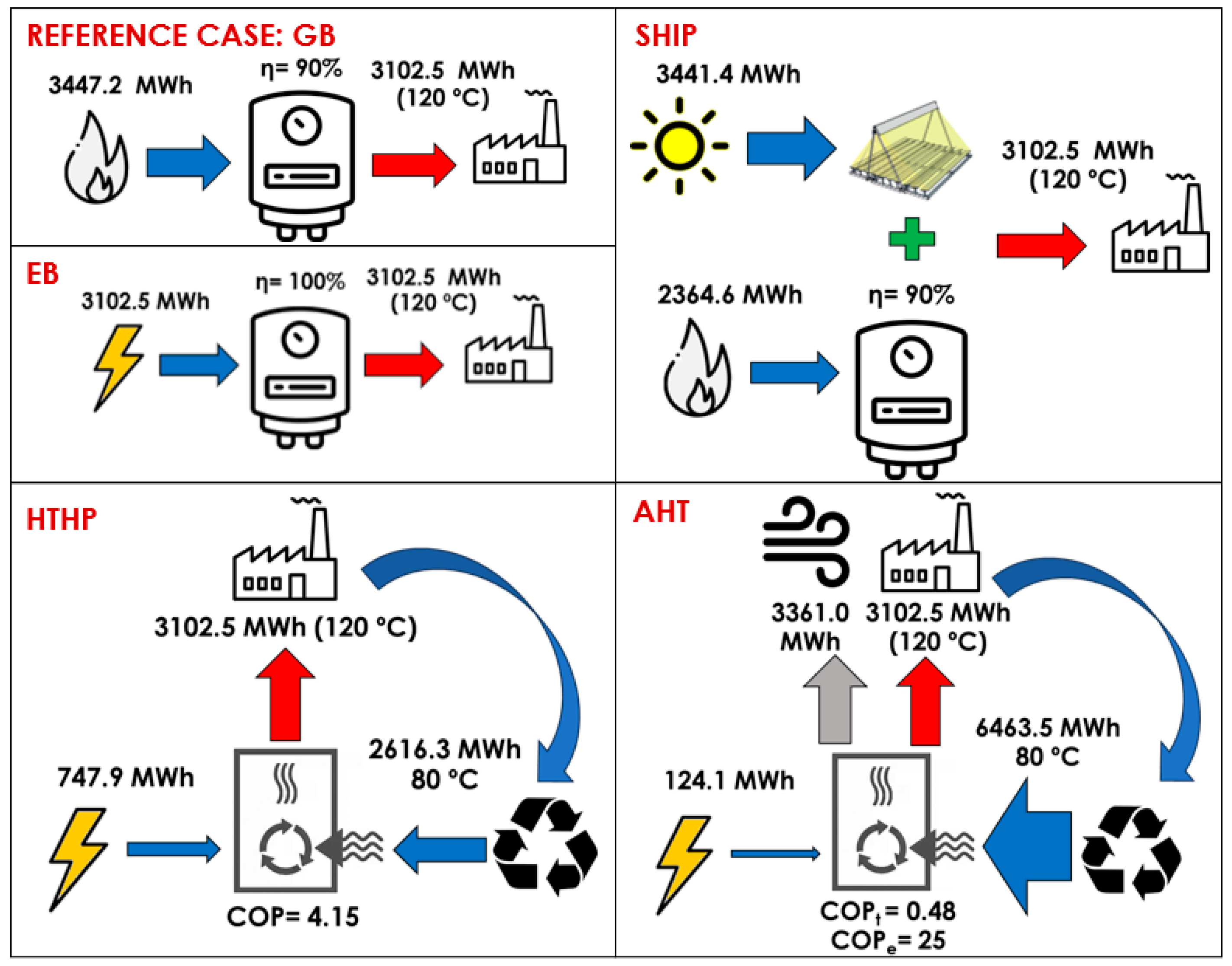
2.1. Technologies Addressed

The reference scenario considered in this study is the gas boiler (GB) case, which is the most common alternative in industry. Figure 1 shows the different technologies that were analyzed and compared with the GB on an annual basis. The alternatives addressed are EBs, SHIP systems, HTHPs, and AHTs. GBs and SHIP systems consume natural gas (either totally or as backup), and the remaining technologies consume electricity (EBs, HTHPs, and AHTs). Nevertheless, HTHPs and AHTs also require recovering waste heat. Thus, they are often referred to as Heat Upgrade Technologies (HUTs).

Figure 1 helps to recognize the main differences between the technologies studied in terms of performance and energy sources. Although HTHPs consume more electrical power than AHTs, they also require less waste heat and do not need to dissipate heat to the ambient. AHTs present the main advantage of consuming a very small amount of electricity. SHIP systems are not self-sufficient since there is practically no useful heat that can be produced in days with minimal direct normal irradiation. Thermal energy storage is still to be proven from an economic point of view in this specific temperature range. Thus, SHIP systems require a backup, which, in this case, is a GB. Finally, EBs consume more electricity than HTHPs or AHTs, but they have the main advantage of their simplicity and relatively low Capital expenditures (CAPEX) compared to the HTHPs or AHTs.

Three potential waste heat recovery temperatures (T_source,in) were considered: 60, 80, and 100 °C. Luberti et al. [38] recently estimated the waste heat availability in the European Union and pointed out that 60 °C is available in the food industry for grain milling, and 80 °C is available in the dairy pasteurization processes of the food industry. Waste heat temperatures of around 100 °C are scarcer [38] but can be found in sugar refining processes (95 °C) or in the canning of fruits or vegetables (120 °C). The exhaust gases in coal-fired power plants (128 °C) could also be potentially recovered to reach this waste heat temperature.

Table 1. Overall simulation matrix in each country.

		Process Heat Temperature: 120 °C			Process Heat Temperature: 150 °C
	Waste Heat Temperature (°C)	60	80	100	60	80	100
Technology	GB
	EB
	SHIP
	HTHP
	AHT

summarizes the different scenarios that were assessed. To produce steam at 120 °C and 150 °C, HTHPs and AHTs cannot work with a heat source at ambient temperature; they both require a minimum waste heat temperature. HTHPs have a wider operation temperature range, considering that the pressure ratios are not too high and that the performance remains high enough with respect to EBs. The performance of AHTs is site-dependent since they have to dissipate heat to the ambient. In order to reach 120 °C with single-effect AHTs, only waste heat at 80 °C and 100 °C is assumed to be technically feasible. To reach 150 °C, the only option with single-effect AHTs would be to recover waste heat at 100 °C.

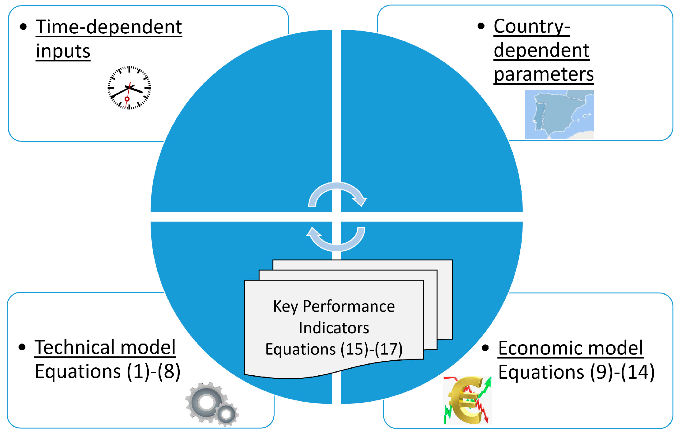
2.2. Modeling Approach, Parameters, and Inputs

The techno-economic analysis depends on the following points, as illustrated in Figure 2:

• Time-dependent inputs such as the thermal demand;
• Country-dependent parameters (e.g., energy prices);
• Technical model;
• Economic model;
• Key Performance Indicators (main outputs such as the payback period).

2.2.1. Time-Dependent Inputs

The time-dependent inputs refer mainly to ambient conditions, such as the hourly ambient temperature or the mean hourly global irradiance on a horizontal surface. The thermal demand Q_demand(t) is also an input. The thermal demand is 500 kW, 16 h/day (from 06:00 to 22:00), seven days/week, all year long. This leads to 5840 h/year. This demand corresponds to the median of the 102 case studies of industrial HTHPs reported in the IEA HPT Annex 48 [39]. High-capacity factors generally lead to lower payback periods [40], so the assessed technologies could potentially reach lower payback periods if applied in industries that allow for more than 6000 h of operation per year.

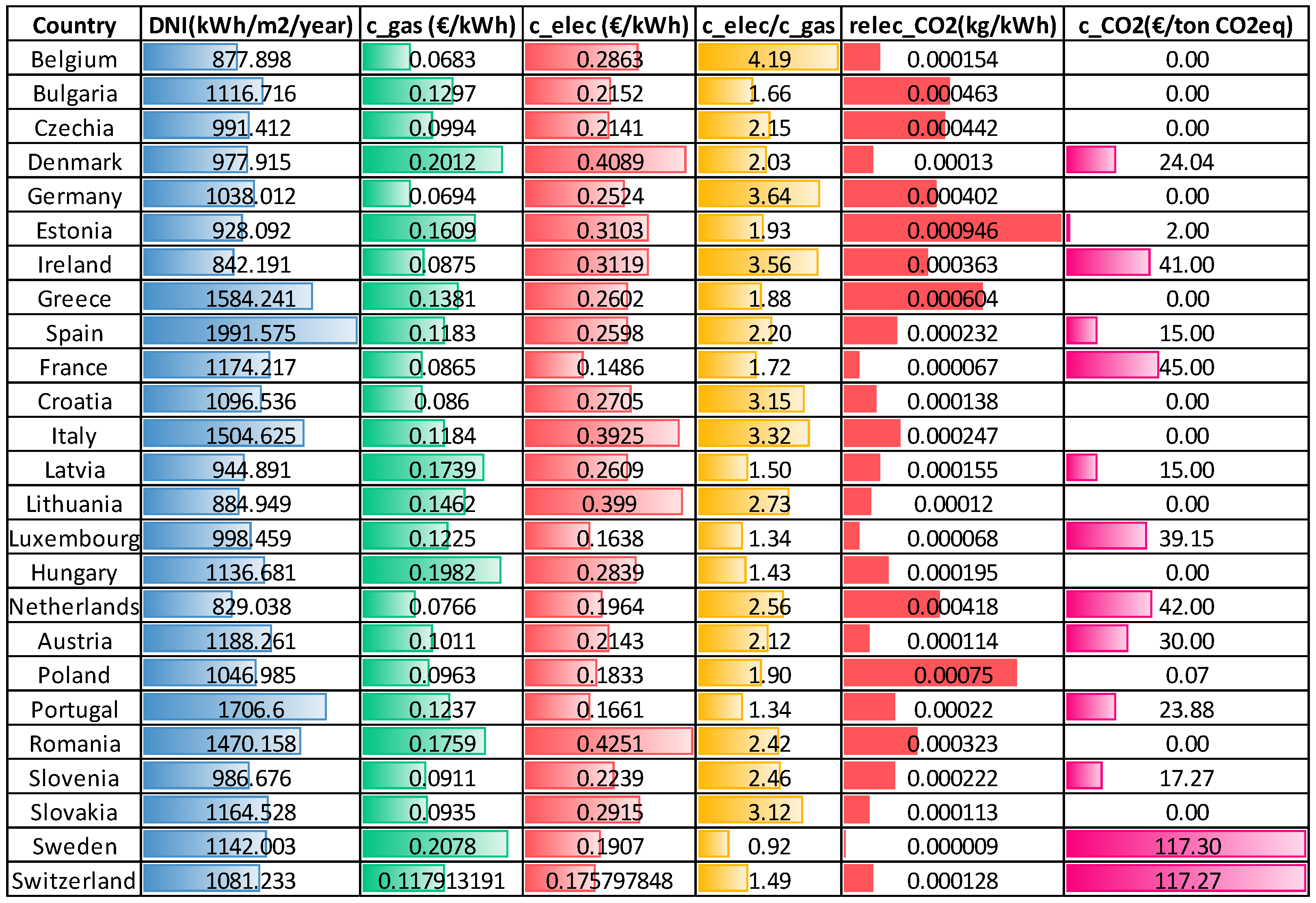
2.2.2. Country-Dependent Parameters

The model also requires country-dependent parameters (Figure 3), such as the cost of gas and electricity in each country. The study covers European countries. The energy costs were obtained from the EUROSTAT database (year 2022) [41], as in recent techno-economic assessments [10]. Although the prices include all taxes and levies, in practice, real prices can differ significantly, even in the same country, depending on the size of the industry, the electricity or gas tariff, etc. For this reason, a parametric study is performed in Section 3.1. The CO₂ emissions of the electricity consumption in each country [40] and the cost of these emissions [42] are included in Figure 3.

Several European countries are not included in Figure 3 as all the country-dependent data were unavailable. This is the case of Liechtenstein, Serbia, and Ukraine, among others.

2.2.3. Technical Model

The reference scenario in this study is the GB case. Depending on its efficiency (η_GB = 0.9 [4]), the corresponding annual gas consumption can be evaluated by Equation (1):

$$W_{annual\_gas,GB}=\frac{Q_{annual\_demand}}{{\eta }_{GB}}=\frac{{\int }_0^{1year}{Q}_{demand}\left(t\right)dt}{{\eta }_{GB}}$$

(1)

In the simulation of the SHIP system, part of the demand is covered with solar energy, and part is fulfilled with a natural gas boiler. In this scenario, Equation (2) is employed to obtain the annual gas consumption. All the thermal demand in this case is not satisfied by the GB since part of the heat is supplied by the solar field. In Equation (2), the net heat provided by the solar installation (Q_{net_solar_heat}) was obtained using the SHIPCAL model [43].

$$W_{annual\_gas,SHIP}=\frac{Q_{annual\_demand}-Q_{net\_solar\_heat}}{{\eta }_{gas\_boiler}}$$

(2)

Finally, the consumption of electricity is calculated with Equations (3)–(5) for the HTHP, AHT, and EB cases, depending on their efficiency.

$$W_{annual\_elec,HTHP}=\frac{Q_{annual\_demand}}{COP\_HTHP\left(T_{source,in}\right)}=\frac{{\int }_0^{1year}{Q}_{demand}\left(t\right)dt}{68.455·{({\mathrm{T}}_{\mathrm{s}\mathrm{i}\mathrm{n}\mathrm{k},\mathrm{o}\mathrm{u}\mathrm{t}}-{\mathrm{T}}_{\mathrm{s}\mathrm{o}\mathrm{u}\mathrm{r}\mathrm{c}\mathrm{e},\mathrm{i}\mathrm{n}})}^{-0.76}}$$

(3)

$$W_{annual\_elec,AHT}=\frac{Q_{annual\_demand}}{{COP}_{el,AHT}}=\frac{{\int }_0^{1year}{Q}_{demand}\left(t\right)dt}{25}$$

(4)

$$W_{annual\_elec\_EB}=Q_{annual\_demand}$$

(5)

The electrical consumption of the HTHP depends on its Coefficient of Performance (COP) [6]. Equation (3) assumes a mean value among different HTHP commercial units. The electrical COP of the AHT system including all the external heat carrier fluid pumps was assumed to be equal to 25, based on a recent analysis made for a 200 kW system [44]. Finally, the EB electrical consumption is the same as the thermal demand since the thermal efficiency equals 1.

For a supply temperature of 120 °C, the COP of the HTHP is 3.05, 4.15, and 7.02 for the three assessed waste heat temperatures T_source,in of 60 °C, 80 °C, and 100 °C, respectively. For a supply temperature of 150 °C, the COP of the HTHP is 2.24, 2.71, and 3.50 for T_source,in values of 60 °C, 80 °C, and 100 °C, respectively.

HTHPs and AHTs require electrical energy consumption, but they also require waste heat, as can be obtained from Equations (6) and (7), respectively. Compressor thermal losses of 35% have been assumed in Equation (6).

$$Q_{annual\_source,HTHP}=W_{annual\_elec\_HTHP}·\left({\phi }_{comp}-1\right)+Q_{annual\_demand}$$

(6)

$$Q_{annual\_source,AHT}=\frac{Q_{annual\_demand}}{{COP}_{th,AHT}}=\frac{Q_{annual\_demand}}{0.48}$$

(7)

In Equation (7), a mean COP_th of 0.48 was assumed for the AHT, independent of the operating point, since the AHT will operate with large driving temperature differences, for which the thermal COP is practically constant, as experimentally confirmed [45]. The AHT, in particular, also has to dissipate heat to the ambient, as expressed in Equation (8):

$$Q_{annual\_amb,AHT}=Q_{annual\_source,AHT}-Q_{annual\_demand}$$

(8)

2.2.4. Economic Model

The annual Operating Expenditures (Equation (9)) include the Operating and Maintenance (O&M) costs (Equation (10)), the cost of the energy consumption (Equation (11)), and the CO₂ emissions (Equation (12)). Such equations refer to year 1 only. For long-term financing periods as in the present study (20 years), a discount analysis is the most accurate approach since it includes both the eventual increase in the energy costs due to inflation and the opportunity costs (discount rate).

Table 2. Parameters of the economic analysis.

Parameter	Value
Analysis period	20 years [10,13,15,24,46]
Discount rate (d)	5% [10,47]
Inflation on gas (igas)	3% [24]
Inflation on electricity (ielec)	3% [24]
Specific cost of GB (cgas_boiler)	70 EUR/kW [48]
Specific cost of HTHP (cHTHP)	700 EUR/kW [30]
Specific cost of SHIP system (cSHIP)	300 EUR/m2 [12]
Specific cost of EB (cEB)	120 EUR/kW [48,49]

shows the economic parameters that were adopted in this study.

$$C_{OPEX,Y1}=C_{O\&M,Y1}+C_{energy,Y1}+C_{CO2,Y1}$$

(9)

$$C_{O\&M,Y1}={0.02·CAPEX}_{scenario}$$

(10)

$$C_{energy,Y1}=W_{annual\_gas}·c_{gas}+W_{annual\_elec}·c_{elec}$$

(11)

$$C_{CO2,Y1}=\left(W_{annual\_gas}·r_{gas\_CO2}+W_{annual\_elec}·{r_{elec\_CO2}·c}_{elec}\right)·c_{CO2}$$

(12)

The Capital Expenditures (CAPEX) value for each scenario was calculated assuming the specific costs indicated in Table 2. The specific cost for each technology is relatively conservative since the values that were selected are mean values of what is reported up-to-date in the published literature.

The CAPEX of the AHT includes a fixed installation cost of 500 EUR/kW, plus a variable term, which is case- and country-dependent since the heat dissipation to the ambient is more critical in warm climates. The CAPEX values were estimated considering that larger heat exchangers are needed in warmer climates for the same temperature lift between the waste and process heat. The total CAPEX, including installation, was obtained using the characteristic equation method [44] to estimate the necessary heat transfer area, yielding values in the range from 765 to 1226 EUR/kW, depending on the country and the operating temperatures.

With the discount method, the yearly costs increase due to inflation, and the future expenses are traced back to the Net Present Value of money (NPV) by considering the market discount rate (d). For any year Y_n, the energy costs were calculated as indicated in Equation (13), assuming that they are paid at the end of each year [50], and by applying the present worth function [50] to address both inflation and opportunity costs. Equation (14) represents the overall OPEX paid at the end of year Y_n, including the energy, O&M, and CO₂ costs.

$$C_{energy,Yn}=C_{gas,Y1}\times \frac{{\left(1+i_{gas}\right)}^{n-1}}{{\left(1+d\right)}^n}+C_{elec,Y1}\times \frac{{\left(1+i_{elec}\right)}^{n-1}}{{\left(1+d\right)}^n}$$

(13)

$$C_{OPEX,Yn}=C_{energy,Yn}+\frac{c_{O\&M,Y1}}{{(1+d)}^n}+\frac{c_{CO2,Y1}}{{(1+d)}^n}$$

(14)

2.2.5. Key Performance Indicators

In order to compare the different scenarios, several Key Performance Indicators (KPIs) were identified and calculated.

Two of the indicators reflect the cost of heat production. For new installations (green-field), the Net Present Value (NPV) of all of the project costs (Equation (11)) represents the total money paid, either for the initial CAPEX or for the annual OPEX during the n years of service life. The Levelized Cost of Heat (LCOH) (Equation (12)) is the total cost per unit of heat generated (EUR/kWh). Basically, both indicators reflect the individual cost of each scenario, although the LCOH relates this cost to the total, discounted heat production [32].

$${NPV}_{all\_costs\_scenario}={CAPEX}_{scenario}+\sum _{n=1}^{n=20years}{C}_{OPEX,Yn}$$

(15)

$${LCOH}_{scenario}=\frac{{CAPEX}_{scenario}+\sum _{n=1}^{n=20years}{C}_{Yn}}{\sum _{n=1}^{n=20years}\frac{Q_{annual\_demand}}{{(1+d)}^n}}$$

(16)

The LCOH or the NPV_{all_costs} provide useful information to determine which technology is less expensive given all the underlying costs. Nevertheless, in a retrofit situation (brown-field), the industry will not likely replace their current gas boilers unless payback periods below 3 to 4 years are obtained (short-term investment).

Thus, some additional indicators were calculated to study if replacing the current industrial gas boilers is economically feasible. For instance, Equation (13) helps obtain the NPV of replacing the GB with any of the assessed alternatives. This expression can be represented graphically as a function of time, as presented later in the Results and Discussion Section.

$${NPV}_{replacement\_scenario}(n)={-CAPEX}_{scenario}+\sum _{n=1}^n{(C}_{Yn,ref}-C_{Yn,scenario})$$

(17)

By definition, the discounted Payback (PB) is the number of years (n) necessary to obtain an NPV with Equation (13) equal to zero. The PB should be lower than the service life of the installation (20 years). The overall benefit can be obtained by solving Equation (13) for n = 20 years.

The model was programmed in MATLAB R2022b. Most of the underlying equations are solved directly, whereas the PB was determined using the vpasolve function. The governing equations are solved for each country given the country-dependent parameters summarized in Table 2.

3. Results

Section 3 presents the results from a local to a global scale. For this reason, in the first place, the results are analyzed more thoroughly for Spain, which is potentially the most interesting of all the studied scenarios, given the high solar radiation and the relatively favorable energy prices. In particular, the chosen location is Almería, with an annual Direct Normal Irradiation (DNI) of 1992 kWh/m²/year. The different technologies are compared in Section 3.1 from an energy, economic, and environmental point of view.

The overall results are discussed afterward on a European level, depending on the energy prices of each country and their CO₂ emission rates. This analysis is performed for process heat temperatures of 120 °C and 150 °C in Section 3.2 and Section 3.3, respectively.

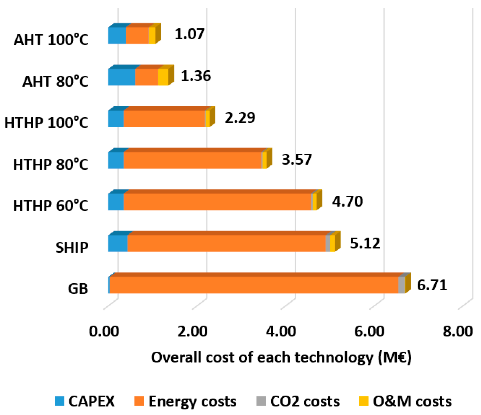
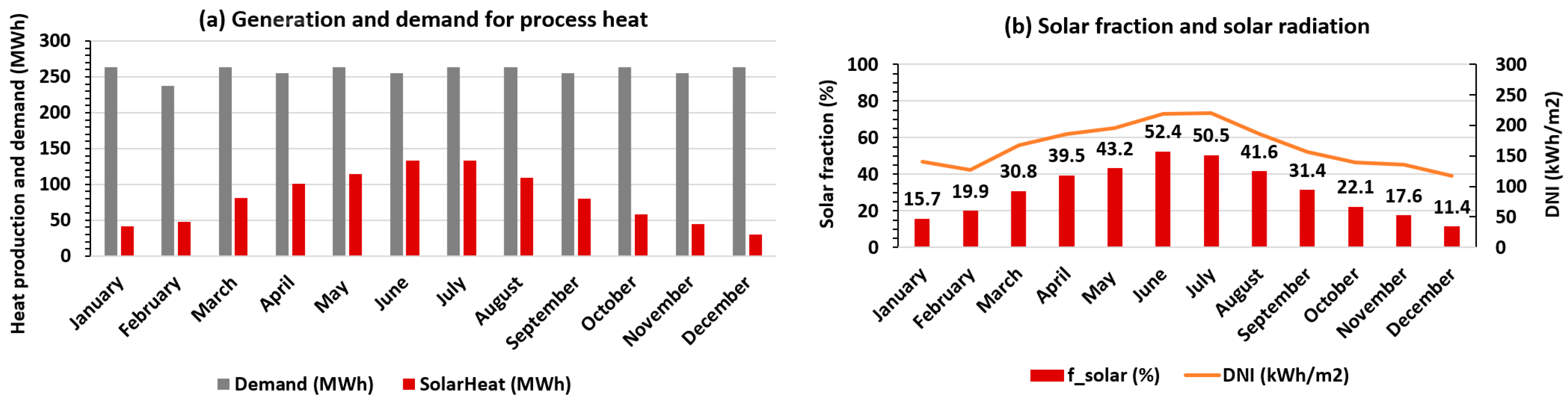
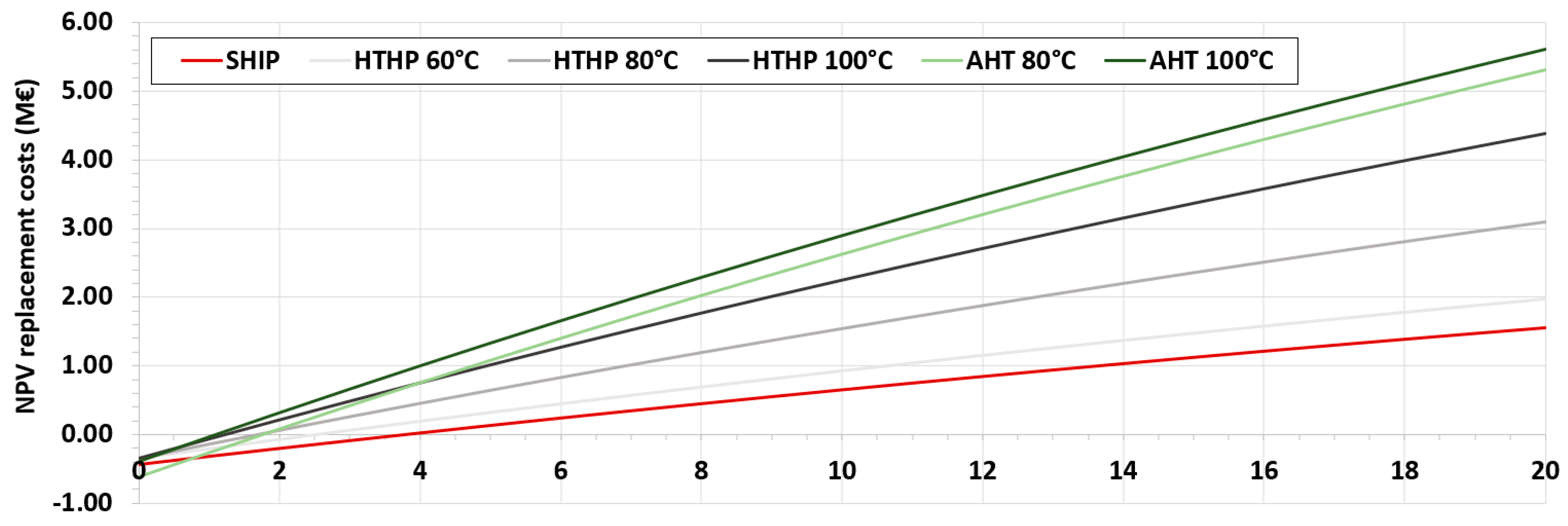
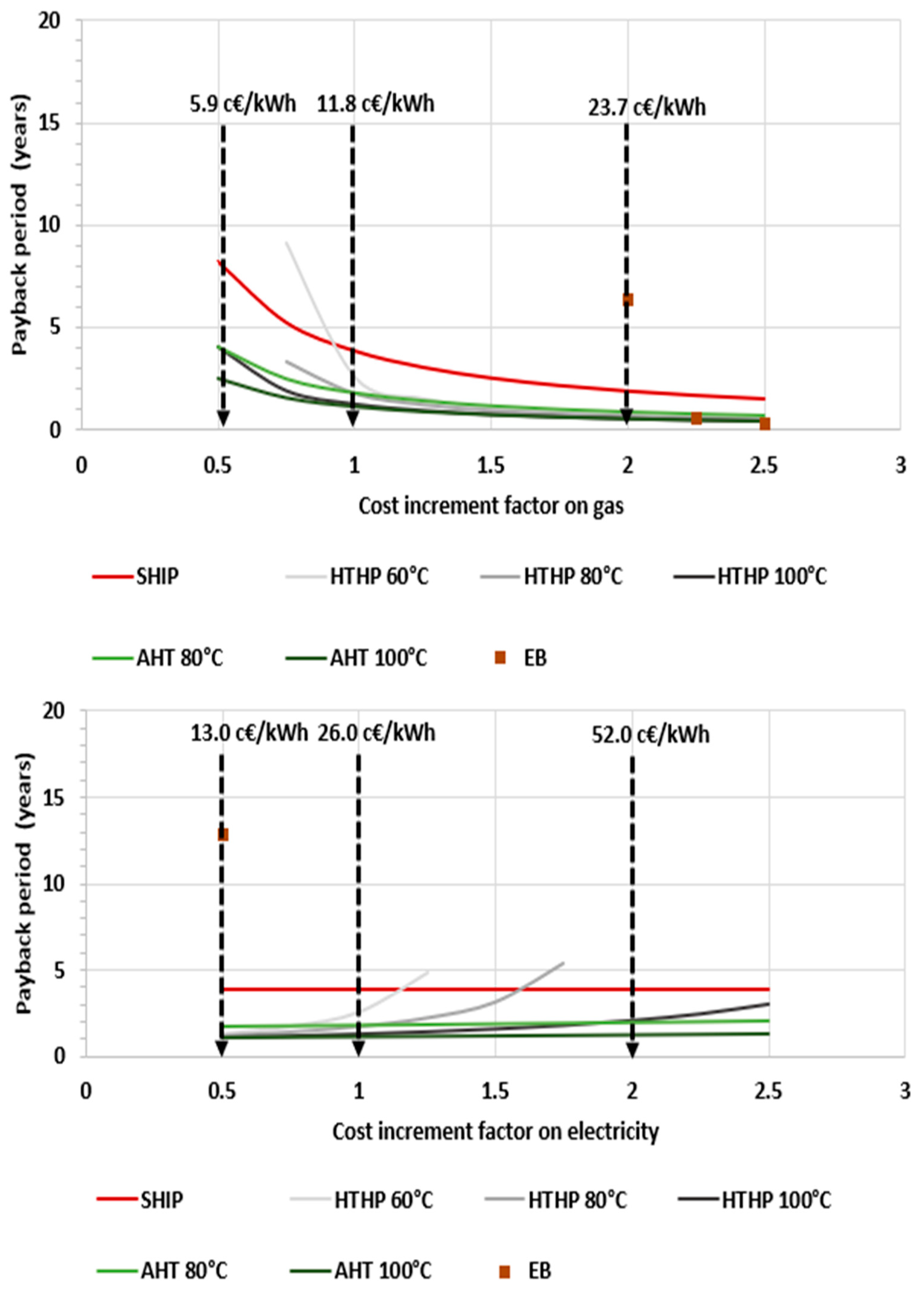
3.1. Detailed Results for Spain for Process Heat Generation at 120 °C

The overall cost obtained with Equation (15) is illustrated in Figure 4. Only the economically feasible scenarios are represented, or in other words, the scenarios where the CAPEX can be recovered before 20 years. For this reason, the EB case is not represented in Figure 4. The most expensive scenario is with the GB, yielding a total cost of 6.71 M€. The lowest total cost is obtained with the AHT (1.36 M€), followed by the HTHP scenarios. For both technologies, the higher the waste heat temperature, the more economic since the system efficiency is higher. The SHIP system involves a total cost of 5.12 M€, which is relatively close to the HTHP 60 °C case (4.70 M€).

Figure 5a represents the monthly thermal demand (grey histogram). The demand is practically the same every month, given that every day follows the same schedule and that the only monthly difference is the number of days per month. The net solar heat (in red) reaches its maximum in summer when the maximum DNI is reached (Figure 5b, orange curve). SHIP systems are generally sized for an annual solar fraction of around 30% [25]. The collectors (1728 m²) were sized to reach this value (30%). For other countries of Europe, the same collector surface was kept in order to study the same system in all locations. Furthermore, it would be necessary to increase significantly the collector surface in regions with low DNI in order to reach this value without any thermal energy storage system, thus increasing the investment cost.

The annual CO₂ emission savings are illustrated in Figure 6. The reference is the GB scenario, which emits around 807 tons/year. The absolute CO₂ emissions are consequently 807 tons/year minus the avoided emissions indicated in Figure 6. The AHT scenarios avoid more CO₂ emissions, followed by the HTHP, due to their COP. The SHIP system, sized for 31% of solar fraction, would avoid 253 tons CO₂/year. More collectors could be potentially added, but the total cost (Figure 4) would increase substantially. At the same time, the payback would presumably decrease, given that part of the solar field would have to be defocused in summer to avoid producing more heat than demanded.

Figure 7 provides useful information to determine if replacing the current industrial gas boilers with other technologies is economically feasible (retrofit situation). After 20 years, and with the energy prices of the EUROSTAT 2022 database, several of the technologies lead to positive NPV values. The highest absolute benefit is obtained with the AHT, followed by the HTHP. The payback periods are relatively low, and generally, all before four years. Nevertheless, the key point is that waste heat should be available at a minimum of 60 °C for the HTHP or at 80 °C for the AHT. The detailed values of the payback period are discussed in the following Section 3.2 on a European level.

Given that the main uncertainty in the techno-economic analysis is the cost of electricity and gas, which are very variable, a specially devoted parametric study is performed in Figure 8. The inflation rate of gas and electricity was kept equal to 3%, but a scale factor was introduced with respect to the energy costs of 2022. This scale factor is from 0.5 up to 2.5, with increments of 0.25. This implies absolute costs of gas in the range from 5.9 to 23.7 c€/kWh, and 13.0 to 52.0 c€/kWh for electricity. PBs higher than the service life of the installations (20 years) have not been represented.

As could be expected, the economic feasibility of SHIP systems only depends on the cost of gas. For gas costs below 11.8 c€/kWh, SHIP systems can lead to payback periods below four years.

For most of the technologies, the higher the reference energy cost (gas) and the lower the electricity cost, the lower the payback. Electric Boilers would only be feasible in Spain in scenarios with very high gas costs (>23.7 c€/kWh) or with very low electricity prices (<13.0 c€/kWh). AHT systems are less sensitive to the price of electricity, given their high COP_el.

HTHPs have a wider operating range than AHT, but given their efficiency, their economic feasibility is strongly dependent on the electricity cost, particularly for low waste heat temperatures. For instance, with waste heat temperatures of 60 °C, the HTHP can only reach PBs below 4 years where the electricity cost remains below 30.29 c€/kWh.

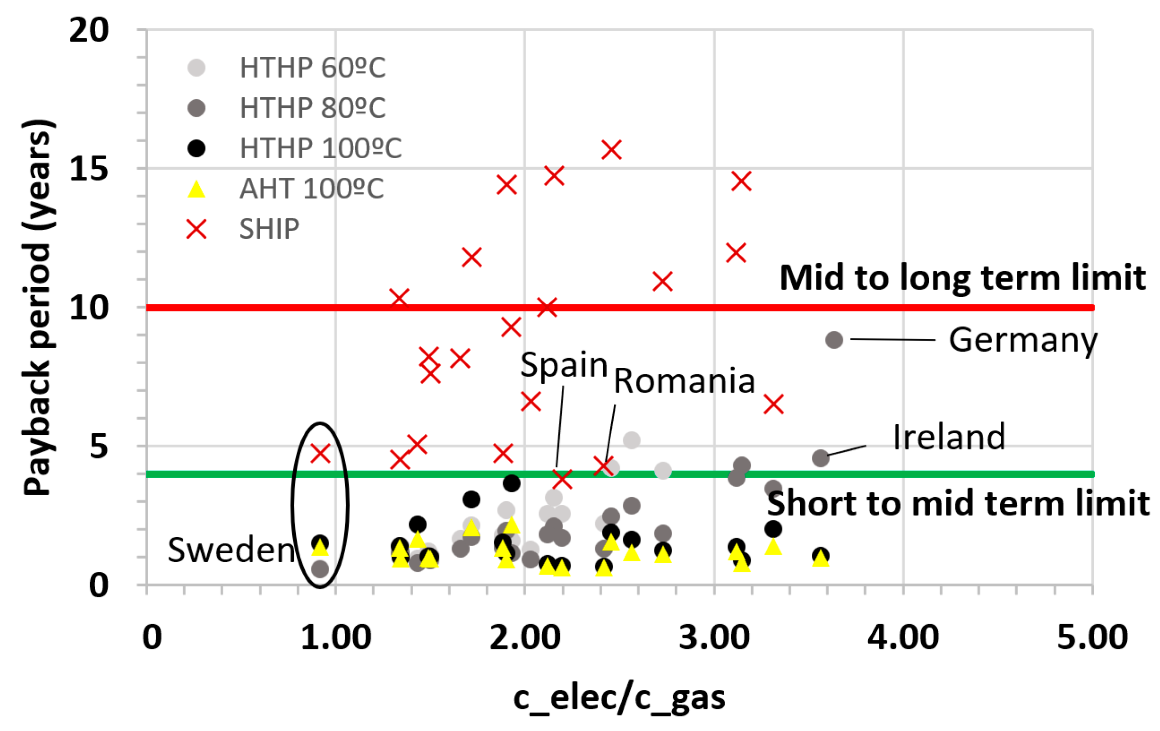
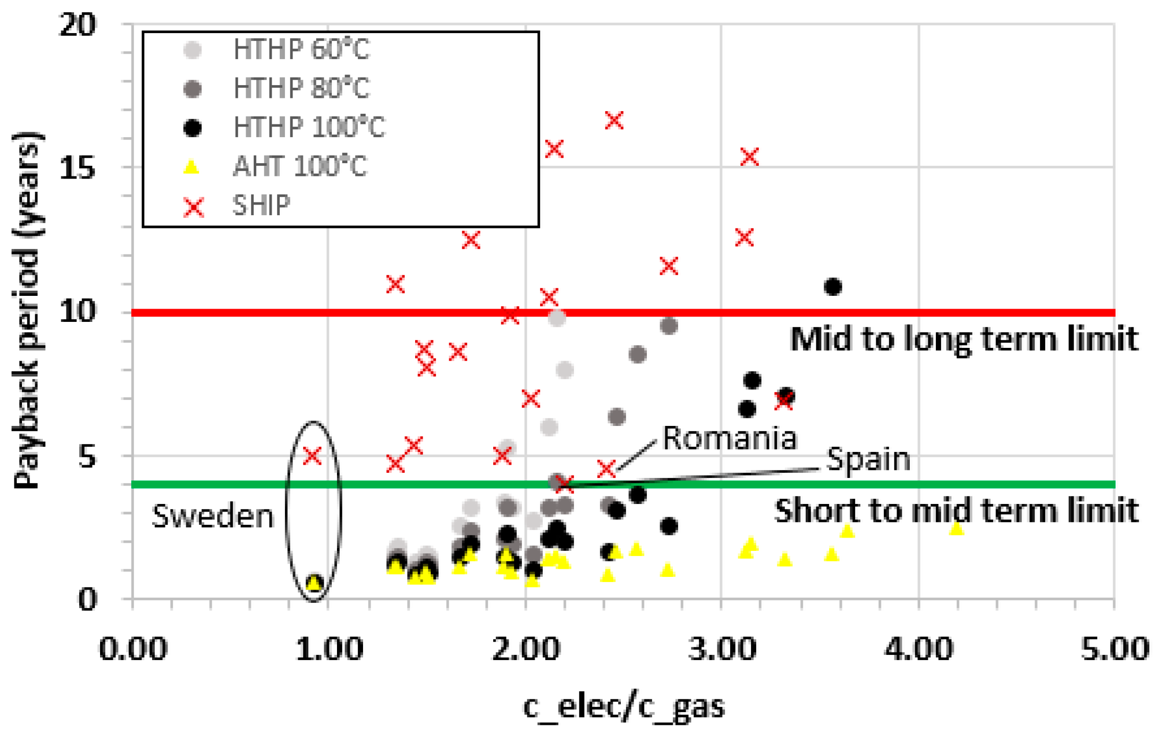
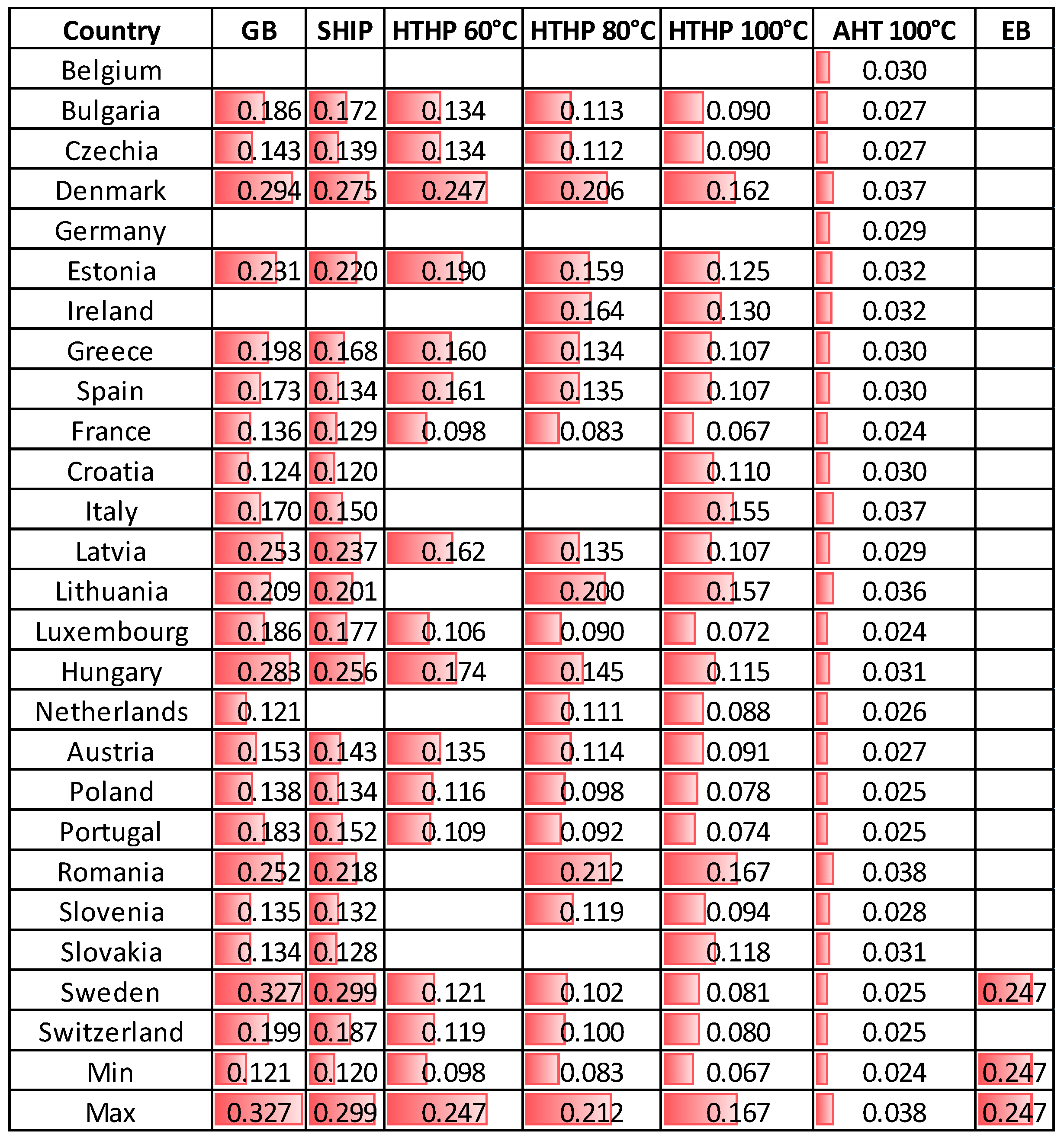
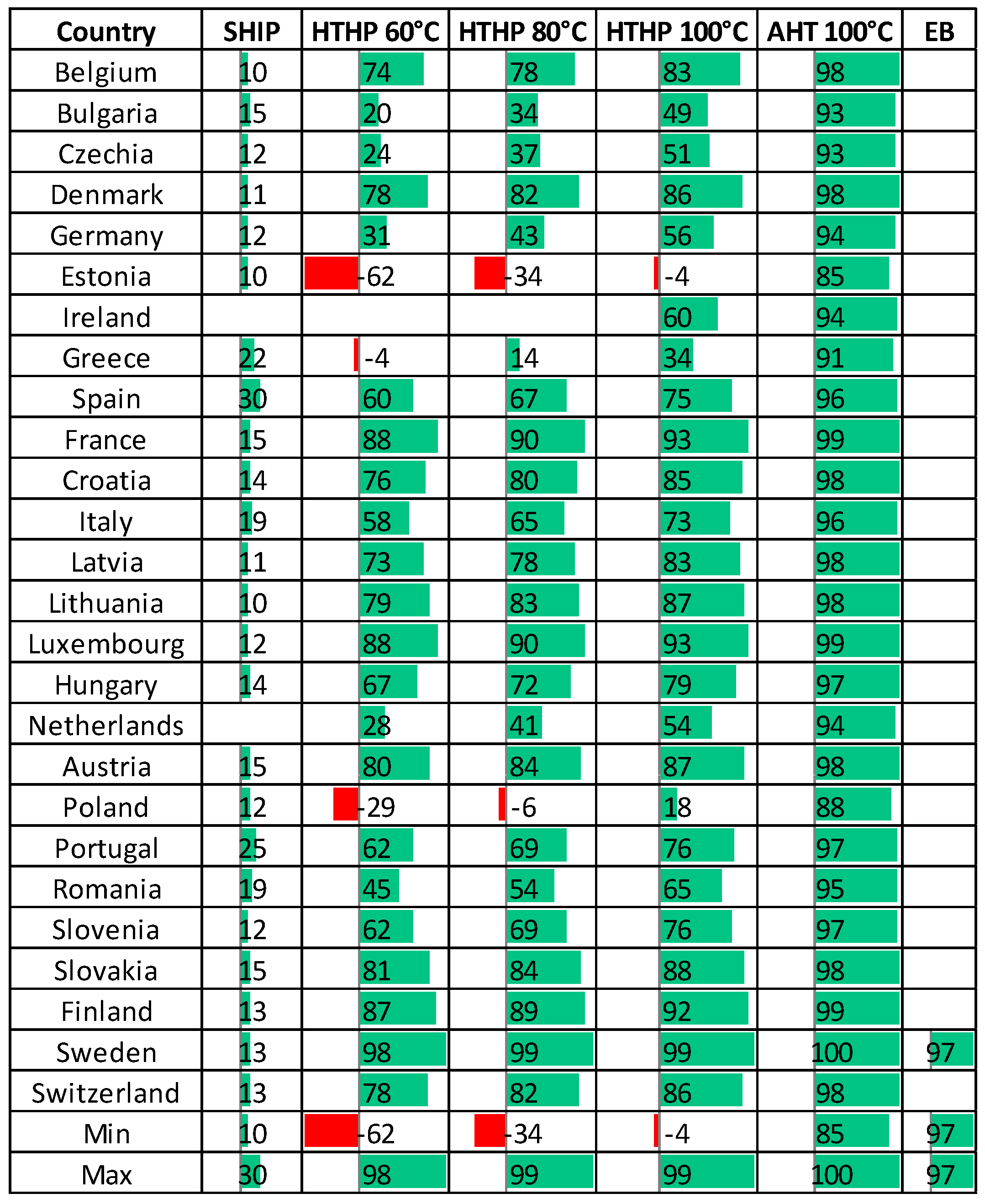
3.2. Overall Results in Europe for Process Heat Generation at 120 °C

The main explanation for the overall European results relies on system efficiencies and on the country-dependent parameters listed in Figure 3. Regarding the SHIP performance, the energy source (DNI) is also a key factor. The price ratio between electricity and gas is often used as an indicator of the market attractiveness for electric-driven HTHPs [1,51], which replace gas consumption with electricity consumption. Given the low cost ratios, Sweden is, in principle, the best-positioned country for electrically-driven systems. At the same time, Belgium presents the highest electricity-to-gas cost ratio and seems less attractive for systems that replace the consumption of gas with electricity. Regarding the CO₂ emissions per every kWh of electricity consumed, Estonia and Poland are clearly the two countries with more CO₂ emissions in their electricity production due to higher usage of fossil fuels, and this has a clear impact later in the CO₂ emission reductions that electrically driven technologies can achieve.

Figure 9 shows the payback periods that are obtained for the different scenarios where the investment is economically feasible (PB lower than 20 years). For instance, the EB case does not recover the initial investment in any country except Sweden, given its low electricity-to-gas cost ratio. However, considering the avoided CO₂ emissions, even if the payback period is very low, HTHPs and AHTs seem to be overall more beneficial than EBs. In some countries such as Belgium, with the current energy prices, only the most efficient HUTs (with waste heat above 80 °C) are economically feasible.

Industries are generally more willing to incorporate new technologies when they involve short-term investments (PB values below four years approximately). These values can be potentially obtained in most of the countries using AHTs and HTHPs. Some exceptions are countries such as Germany or the Netherlands in the HTHP 60 °C scenario (lower COP and relatively high electricity-to-gas cost ratio).

Figure 10 represents the PB values of Figure 9 as a function of the electricity-to-gas cost ratio. Short-term investments are achieved easily with both AHTs or HTHPs recovering waste heat at 100 °C. However, the limit of 4 years is reached with the HTHP 80 °C for cost ratios of a maximum of 3.5, and for the HTHP 60 °C, the limit is a cost ratio of around 2.8.

The SHIP scenario requires specific attention since the payback periods are not so directly correlated with the electricity-to-gas cost ratio. Their economic benefit depends mainly on the CAPEX, the price of gas, and the DNI. Figure 11 represents the payback period of the different countries as a function of the DNI. Although the payback is also dependent on the price of gas, in general, all countries with DNI values above 1400 kWh/m²/year lead to payback periods between 4 and 5 years, which are close to short-term investments. Given the high inflation on gas between 2021 and 2023, many new SHIP systems are actually being built in these countries. Romania is an interesting case where the DNI value is lower than in Portugal and Spain, but the payback period is similar. The reason for this is that the price of gas is around 18 c€/kWh, compared to 12 c€/kWh in Portugal and Spain.

Figure 12 illustrates the LCOH of the different technologies whenever the investment is economically feasible. The lowest LCOH values are obtained with AHTs (ranging from 2.1 to 4.2 c€/kWh) depending on the country, followed by the HTHPs (3.8 to 19 c€/kWh). The SHIP LCOHs are in the range of 11.9 to 30.9 c€/kWh, which is close to the LCOHs values of GBs (10.0 to 34.1 c€/kWh). However, in countries with a high DNI, such as Spain, the LCOH of SHIP systems can reach values of around 13.2 c€/kWh, which is lower than 17.3 €/kWh (GB scenario in Spain). As in previous tables, the values of scenarios with payback periods below 20 years are not included. This is the case of Belgium in many scenarios, except for those with waste heat temperatures above 80 °C.

Finally, Figure 13 represents the yearly CO₂ emission savings as a % variation with respect to the GB case. Practically all scenarios help reduce the CO₂ emissions (green color), except for the HTHP with waste heat at 60 °C in Estonia (red color). In Poland, this scenario only reduces the CO₂ emissions by 5%. The reason is that these two countries are among those with higher CO₂ emission rates in their electricity production, as discussed at the beginning of Section 3.2. AHTs, given their high COP_el, can reduce CO₂ emissions from 85 to 100%. This upper value is reached in Sweden, which has very low CO₂ emission rates in electricity production since most of it is produced with hydraulic and nuclear power. HTHPs also enable a significant reduction in CO₂ emissions. With the mean waste heat temperature of 80 °C, the CO₂ emission reduction is in the range from 12% (Poland) to 99% (Sweden).

3.3. Overall Results in Europe for Process Heat Generation at 150 °C

Heat supply at around 150 °C is roughly the current limit of commercial HTHPs. Beyond this temperature, and particularly in the temperature range from 150 to 300 °C, SHIP systems, despite their higher payback periods, remain the best alternative to reduce the carbon footprint of the industry. For AHTs, the highest reported delivery temperature with single effect cycles is 157 °C, and double effect machines with lower efficiencies and higher specific capital costs can be used for supply temperatures up to 180 °C [35].

As inferred from Figure 14, the payback periods of SHIP systems for heat production at 150 °C are very similar to the values obtained for 120 °C since the absorbers are made of evacuated-tube collectors and the additional heat losses are not particularly high for a temperature increase of only 30 °C. Thus, the same conclusions apply for SHIP systems both for 120 and 150 °C. Countries with DNI values above 1400 kWh/m²/year have in general payback periods of around four years.

For the rest of the technologies, the most relevant difference at 150 °C is that AHTs can only work properly with waste heat temperatures of 100 °C, which is less frequent in industry, as discussed previously. Nevertheless, if found, this waste heat temperature would lead to the lowest payback periods with AHTs (0.6 and 2.5 years). With HTHPs, the main advantage is that they are technically and economically feasible even with waste heat temperatures of 60 °C. The payback periods with HTHPs are in the range of 0.6 to 10.9 years. In countries with electricity-to-gas cost ratios below two, payback periods below 1.5 years are generally obtained with HTHPs.

The payback periods can also be better understood for the HUTs as a function of the electricity-to-gas cost ratio (Figure 15). Depending on the waste heat temperature, the payback limit of 4 years can be reached with a different electricity-to-gas cost ratio. For 60–80–100 °C waste heat temperature, the maximum cost ratio to reach the PB limit of four years is 2.20–2.50–3.00.

Figure 16 represents the LCOH, which is obtained with the different technologies. Since the efficiencies are lower than in the 120 °C case, the LCOH of the HUTs is also higher. For instance, the LCOH for the HTHPs now ranges between 6.7 and 24.7 c€/kWh. In the AHT 100 °C case, the LCOH is between 2.4 and 3.8 c€/kWh. Even in Sweden, which is the only country with a feasible payback period for the EB case, its LCOH (24.7 c€/kWh) is higher than for most of the technologies and is only lower than the LCOH of the SHIP system in some specific countries with either low DNI values or very high gas prices.

The percentage reduction in CO₂ emissions is shown in Figure 17 with respect to the GB case. For process heat supply at 150 °C, since the HUTs work under more demanding operating conditions, their efficiencies are lower, and the potential reductions in the emissions are, in general, lower. As also observed in Section 3.2, this is critical in countries such as Estonia or Poland, with high emission rates in their electricity production. In Spain, in the HTHP 80 °C case, the potential CO₂ emission reduction is 67%, whereas for 120 °C, the potential reduction is 78%.

4. Conclusions

This study compares the techno-economic potential of different technologies for steam generation at 120 °C and 150 °C in European industry. As a reference, GBs were used as the most common solution at present. The developed model, implemented in MATLAB, is time- and country-specific since it requires inputs such as the direct normal irradiance and parameters such as the energy prices or indirect CO₂ emissions in the electricity production of each country. For more accuracy, dynamic models including part-load performance are recommended. However, for the objective of the present work, the developed model is sufficient for reaching the following conclusions regarding the situation and perspectives of each technology:

• Despite their simplicity and relatively low CAPEX, EBs are not economically feasible in Europe with the current energy prices, with the single exception of Sweden, which is the country with the lowest electricity-to-gas price ratio.
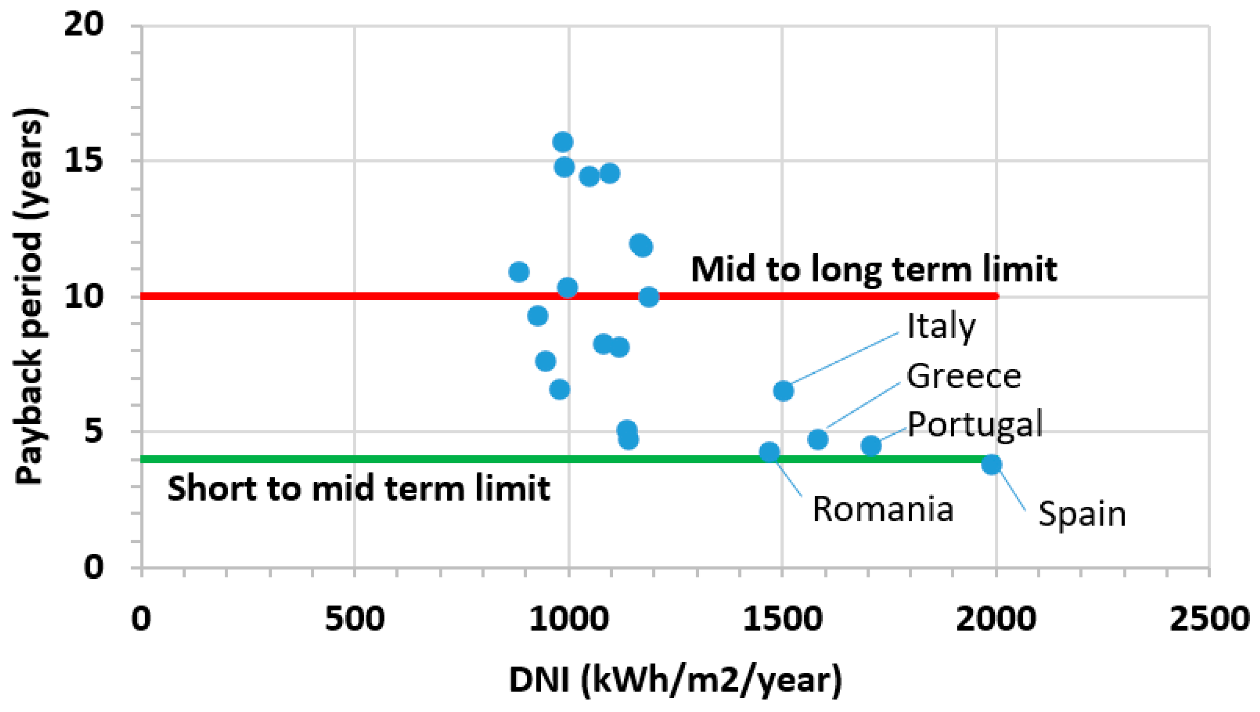
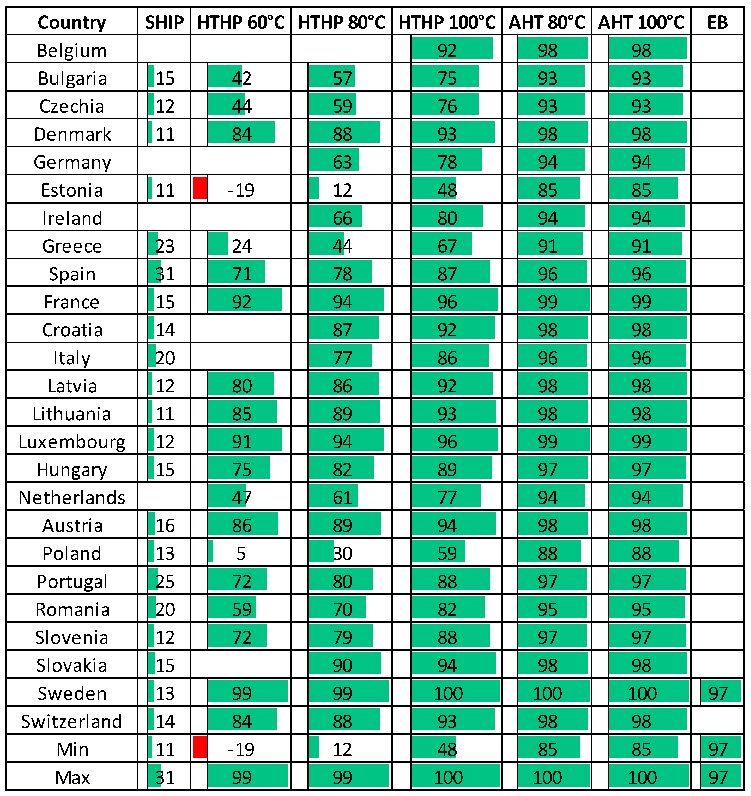
• SHIP systems differ from the other alternatives since they are not self-sufficient. On days with a low DNI, they require a backup, which, in this case, is a GB. In Spain, for instance, an annual solar coverage demand of 31% was reached. The remaining 69% is ensured by a backup GB, which is a significant penalty in terms of the potential reduction in CO₂ emissions. In countries with high DNI values, such as Spain, the SHIP system can reduce CO₂ emissions by 31%, reaching a LCOH of 13 c€/kWh, which is lower than with the GB (17 c€/kWh). In general, countries with DNI values above 1400 kWh/m²/year have, using SHIP systems, PBs of around 4 to 5 years. This is the case in countries such as Greece, Spain, Italy, Portugal, and Romania. SHIP systems can play a key role in reducing the industrial carbon footprint given that they are capable of reaching higher temperatures (150 to 400 °C) than HTHPs or AHTs.
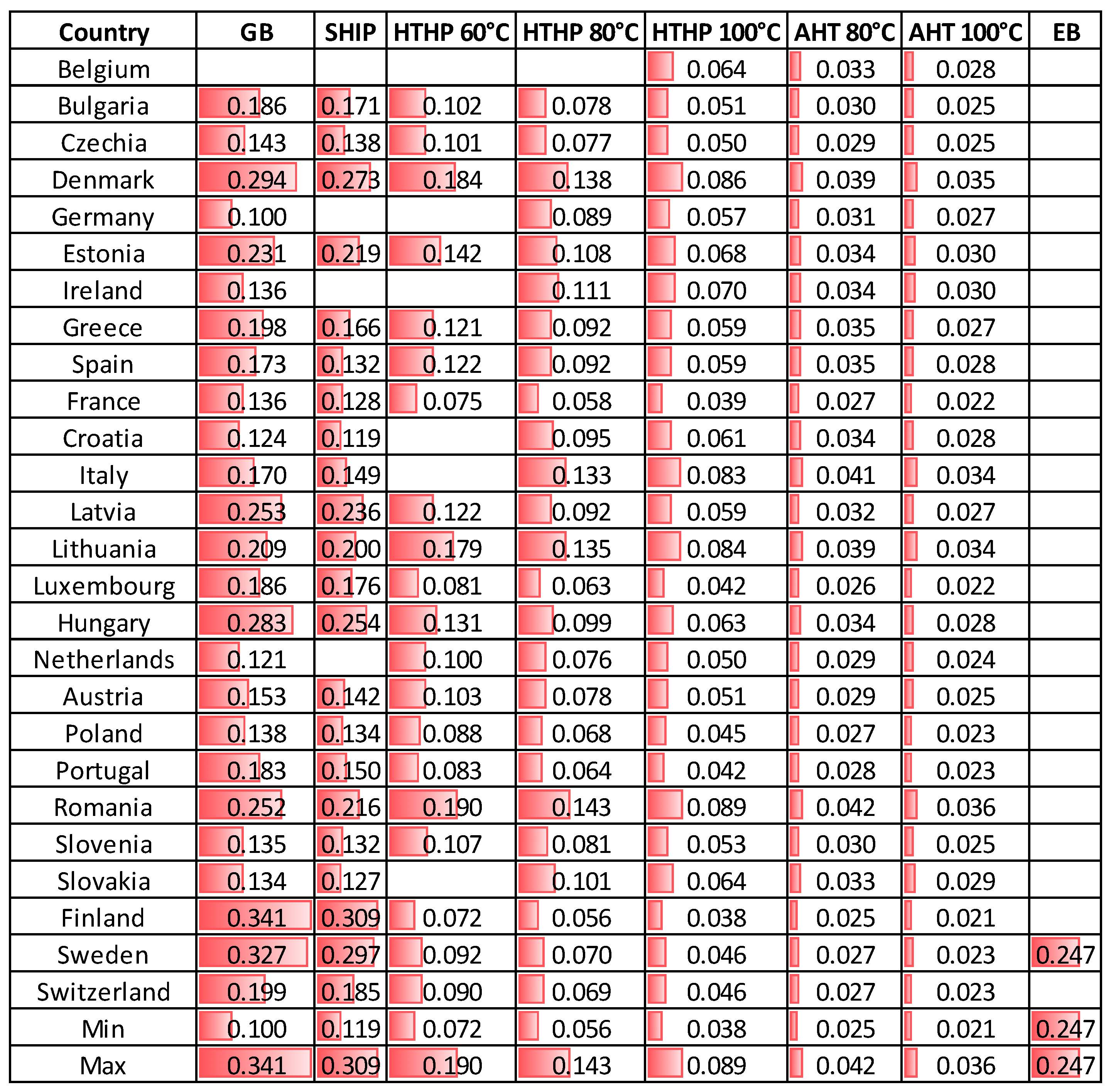
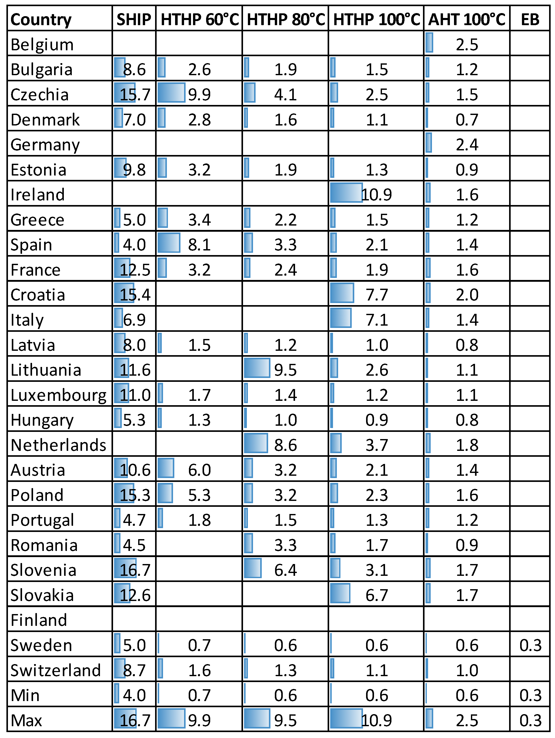
• HTHPs can attain PBs of less than four years for process heat supply temperatures of 120 °C. Their economic feasibility is more sensitive to the electricity cost than AHTs. HTHPs require electricity-to-gas cost ratios of a maximum of 3.5 with waste heat temperatures of 80 °C or a maximum cost ratio of 2.8 if the waste heat is available at only 60 °C. For process heat at 150 °C, if waste heat is available at 60–80–100 °C, the maximum cost ratio is 2.20–2.50–3.00, respectively. For process heat supply at 150 °C, PBs of 0.6 to 10.9 years can be reached in Europe. PBs below 1.5 years can be achieved in countries with electricity-to-gas price ratios below two. This is the case in countries such as Latvia, Hungary, Sweden, and Switzerland.
• AHTs reach the lowest CO₂ emissions, LCOH, and CO₂ emissions. However, the operating temperature ranges are narrower than with the HTHP. For instance, for process heat at 120 °C, the minimum waste heat temperature required is 80 °C, whereas for process heat at 150 °C, waste heat at 100 °C would be required, and this is less frequent in industry. With these temperatures, LCOH values in the range of 2 to 4 c€/kWh could be potentially achieved. In terms of PB values, the range in all European countries is 0.7 to 2.2 years for process heat at 120 °C and waste heat at 80 °C, and 0.6 to 2.5 years for process heat at 150 °C and waste heat at 100 °C.

This techno-economic study also shows that policy measures to limit CO₂ emissions are needed to encourage a faster uptake of heat pump technologies. Recommendations for policy measures include the introduction of financial incentives (e.g., financial support to cover the additional capital costs) and pricing mechanisms to ensure that heat pumps cost less than fossil fuel systems (e.g., exemption from climate policy costs on electricity prices, CO₂ tax on fossil fuels, and participation in the CO₂ emissions trading scheme). These policy measures will vary from country to country, and there are different strategies and energy prices. Policy stability is also important to drive long-term investments and decisions and to ensure that the transition to heat pumps is easy.

As future work, within the PUSH2HEAT project, the integration of HTHPs or AHTs in different industrial demo sites will be explored. The project aims to demonstrate their techno-economic feasibility, supported by real, on-site monitoring data.

References

1. de Boer, R.; Marina, A.; Zühlsdorf, B.; Arpagaus, C.; Bantle, M.; Wilk, V.; Elmegaard, B.; Corberan, J.; Benson, J. Strengthening Industrial Heat Pump Innovation, Decarbonizing Industrial Heat. 2020. Available online: https://sintef.brage.unit.no/sintef-xmlui/bitstream/handle/11250/2764774/WhitePaper_HTHP_InudstrialHeatPump.pdf?sequence=2 (accessed on 17 February 2024).
2. European Commission European Grean Deal Long Term Strategy 2050. Available online: https://ec.europa.eu/clima/eu-action/climate-strategies-targets/2050-long-term-strategy_es (accessed on 17 February 2024).
3. Dadi, D.; Introna, V.; Benedetti, M. Decarbonization of Heat through Low-Temperature Waste Heat Recovery: Proposal of a Tool for the Preliminary Evaluation of Technologies in the Industrial Sector. Sustainability 2022, 14, 12626. [Google Scholar] [CrossRef]
4. Dengler, J.; Köhler, B.; Dinkel, A.; Bonato, P.; Azam, N.; Kalz, D. Mapping and Analyses of the Current and Future (2020–2030) Heating/Cooling Fuel Deployment (Fossil/Renewables). Work Package 2: Assessment of the Technologies for the Year 2012. 2016. Available online: https://energy.ec.europa.eu/system/files/2016-04/Summary%2520WP1%2520and%2520WP2_0.pdf (accessed on 17 February 2024).
5. Fox, D.B.; Sutter, D.; Tester, J.W. The Thermal Spectrum of Low-Temperature Energy Use in the United States. Energy Environ. Sci. 2011, 4, 3731–3740. [Google Scholar] [CrossRef]
6. Arpagaus, C.; Bless, F.; Uhlmann, M.; Schiffmann, J.; Bertsch, S.S. High Temperature Heat Pumps: Market Overview, State of the Art, Research Status, Refrigerants, and Application Potentials. Energy 2018, 152, 985–1010. [Google Scholar] [CrossRef]
7. Office of Energy Efficiency & Renewable Energy. U.S. Manufacturing Energy Use and Greenhouse Gas Emissions Analysis. 2012. Available online: https://www.energy.gov/sites/default/files/2013/11/f4/energy_use_and_loss_and_emissions.pdf (accessed on 17 February 2024).
8. McMillan, C.A.; Ruth, M. Using Facility-Level Emissions Data to Estimate the Technical Potential of Alternative Thermal Sources to Meet Industrial Heat Demand. Appl. Energy 2019, 239, 1077–1090. [Google Scholar] [CrossRef]
9. Kempener, R.; Saygin, D. Renewable Energy in Manufacturing—A Technology Roadmap for REmap 2030; International Renewable Energy Agency (Rena): Abu Dhabi, United Arab Emirates, 2014. [Google Scholar]
10. Kosmadakis, G.; Arpagaus, C.; Neofytou, P.; Bertsch, S. Techno-Economic Analysis of High-Temperature Heat Pumps with Low-Global Warming Potential Refrigerants for Upgrading Waste Heat up to 150 °C. Energy Convers Manag. 2020, 226, 113488. [Google Scholar] [CrossRef]
11. Annex 58-High-Temperature Heat Pumps. Available online: https://heatpumpingtechnologies.org/annex58/ (accessed on 5 May 2022).
12. Ivancic, A.; Mugnier, D.; Stryi-Hipp, G.; Weiss, W. Solar Heating and Cooling Technology Roadmap. Eur. Technol. Platf. Renew. Heat. Cool. 2014, 1–32. [Google Scholar] [CrossRef]
13. Jesper, M.; Schlosser, F.; Pag, F.; Walmsley, T.G.; Schmitt, B.; Vajen, K. Large-Scale Heat Pumps: Uptake and Performance Modelling of Market-Available Devices. Renew. Sustain. Energy Rev. 2021, 137, 110646. [Google Scholar] [CrossRef]
14. Wang, Z. Heat Pumps with District Heating for the UK’s Domestic Heating: Individual versus District Level. Energy Procedia 2018, 149, 354–362. [Google Scholar] [CrossRef]
15. Schlosser, F.; Jesper, M.; Vogelsang, J.; Walmsley, T.G.; Arpagaus, C.; Hesselbach, J. Large-Scale Heat Pumps: Applications, Performance, Economic Feasibility and Industrial Integration. Renew. Sustain. Energy Rev. 2020, 133, 110219. [Google Scholar] [CrossRef]
16. EEP. The Energy Efficiency Index of German Industry: Evaluation Results EEI 2019; 1st Half. 2019; Universität Stuttgart: Stuttgart, Germany, 2019. (In German) [Google Scholar]
17. Tannous, H.; Stojceska, V.; Tassou, S.A. The Use of Solar Thermal Heating in SPIRE and Non-SPIRE Industrial Processes. Sustainability 2023, 15, 7807. [Google Scholar] [CrossRef]
18. IEA SHC Task 49. Available online: https://task49.iea-shc.org/ (accessed on 17 February 2024).
19. IEA Task 64 on Solar Process Heat. Available online: https://task64.iea-shc.org/ (accessed on 17 February 2024).
20. Horta, P. Process Heat Collectors: State of the Art and Available Medium Temperature Collectors; IEA SHC Task 49 Technical Report A.1.3; IEA SHC: Cedar, MI, USA, 2016. [Google Scholar]
21. IEA-ETSAP; IRENA. Solar Heat for Industrial Processes: Technology Brief; International Renewable Energy Agency: Masdar City, United Arab Emirates, 2015. [Google Scholar]
22. Weiss, W.; Spörk-Dür, M. Edition 2022 Global Market Development and Trends 2021 Detailed Market Figures 2020 Solar Heat World Wide; IEA SHC: Cedar, MI, USA, 2022. [Google Scholar]
23. Zhao, Z.; Yuan, H.; Gao, S.; Tian, Y. Comparative Study on Performance and Applicability of High Temperature Water Steam Producing Systems with Waste Heat Recovery. Case Stud. Therm. Eng. 2021, 28, 101622. [Google Scholar] [CrossRef]
24. Meyers, S.; Schmitt, B.; Vajen, K. The Future of Low Carbon Industrial Process Heat: A Comparison between Solar Thermal and Heat Pumps. Solar Energy 2018, 173, 893–904. [Google Scholar] [CrossRef]
25. de Santos López, G. Techno-Economic Analysis and Market Potential Study of Solar Heat in Industrial Processes A Fresnel Direct Steam Generation Case Study. Master’s Thesis, KTH Royal Institute of Technology, Stockholm, Sweden, 2021. [Google Scholar]
26. Vieren, E.; Couvreur, K.; de Paepe, M.; Lecompte, S. Techno-Economic Analysis of High Temperature Heat Pumps: A Case Study. In Proceedings of the 15th International Conference on Heat Transfer, Fluid Mechanics and Thermodynamics (HEFAT2021), Amsterdam, The Netherlands, 25–28 July 2021; pp. 2109–2114. [Google Scholar]
27. Filali Baba, Y.; Ajdad, H.; al Mers, A.; Bouatem, A.; Bououlid Idrissi, B.; el Alj, S. Preliminary Cost-Effectiveness Assessment of a Linear Fresnel Concentrator: Case Studies. Case Stud. Therm. Eng. 2020, 22, 100730. [Google Scholar] [CrossRef]
28. Law, R.; Harvey, A.; Reay, D. Techno-Economic Comparison of a Hightemperature Heat Pump and an Organic Rankine Cycle Machine for Low-Grade Waste Heat Recovery in UK Industry. Int. J. Low-Carbon Technol. 2013, 8, i47–i54. [Google Scholar] [CrossRef]
29. Meyers, S.; Schmitt, B.; Vajen, K. Renewable Process Heat from Solar Thermal and Photovoltaics: The Development and Application of a Universal Methodology to Determine the More Economical Technology. Appl. Energy 2018, 212, 1537–1552. [Google Scholar] [CrossRef]
30. Arpagaus, C.; Bless, F. Techno-Economic Analysis of Steam Generating Heat Pumps for Integration into Distillation Processes. In Proceedings of the 15th IIR-Gustav Lorentzen Conference on Natural Refrigerants, Trondheim, Norway, 13–15 June 2022. [Google Scholar]
31. Ghasemi, M.; Saini, P.; Arpagaus, C.; Bertsch, S.; Zhang, X. Techno-Economic Comparative Analysis of Solar Thermal Collectors and High-Temperature Heat Pumps with PV for Industrial Steam Generation. In Proceedings of the 14th IEA Heat Pump Conference, Chicago, IL, USA, 15–18 May 2023. [Google Scholar]
32. Vieren, E.; Demeester, T.; Beyne, W.; Magni, C.; Abedini, H.; Arpagaus, C.; Bertsch, S.; Arteconi, A.; De Paepe, M.; Lecompte, S. The Potential of Vapor Compression Heat Pumps Supplying Process Heat between 100 and 200 °C in the Chemical Industry. Energies 2023, 16, 6473. [Google Scholar] [CrossRef]
33. Brückner, S.; Liu, S.; Miró, L.; Radspieler, M.; Cabeza, L.F.; Lävemann, E. Industrial Waste Heat Recovery Technologies: An Economic Analysis of Heat Transformation Technologies. Appl. Energy 2015, 151, 157–167. [Google Scholar] [CrossRef]
34. Cudok, F.; Giannetti, N.; Ciganda, J.L.C.; Aoyama, J.; Babu, P.; Coronas, A.; Fujii, T.; Inoue, N.; Saito, K.; Yamaguchi, S.; et al. Absorption Heat Transformer—State-of-the-Art of Industrial Applications. Renew. Sustain. Energy Rev. 2021, 141, 110757. [Google Scholar] [CrossRef]
35. Aoyama, J.; Oikawa, Y. Ebara’s Absorption Heat Pump—Type II Heat Transformer. In Proceedings of the 14th IIR Gustav Lorentzen Conference on Natural Refrigerants, Tokyo, Japan, 7 December 2020. [Google Scholar]
36. Fujii, T.; Nishiguchi, A.; Uchida, S. Development Activities of Low Temperature Waste Heat Recovery Appliances Using Absorption Heat Pumps, Tokyo, Japan. In Proceedings of the International Symposium on Next-Generation air Conditioning and Refrigeration Technology 10, Tokyo, Japan, 17–19 February 2010; pp. 1–8. [Google Scholar]
37. Ma, X.; Chen, J.; Li, S.; Sha, Q.; Liang, A.; Li, W.; Zhang, J.; Zheng, G.; Feng, Z. Application of Absorption Heat Transformer to Recover Waste Heat from a Synthetic Rubber Plant. Appl. Therm. Eng. 2003, 23, 797–806. [Google Scholar] [CrossRef]
38. Luberti, M.; Gowans, R.; Finn, P.; Santori, G. An Estimate of the Ultralow Waste Heat Available in the European Union. Energy 2022, 238, 121967. [Google Scholar] [CrossRef]
39. Jakobs, R.M.; Stadtländer, C. Final Report Industrial Heat Pumps, Second Phase Final Report Authors; IEA Technology Collaboration Programme on Heat Pumping Technologies; International Energy Agency: Paris, France, 2020. [Google Scholar]
40. Lee, A.H.W.; Jones, J.W. Modeling of an Ice-on-Coil Thermal Energy Storage System. Energy Convers Manag. 1996, 37, 1493–1507. [Google Scholar] [CrossRef]
41. EUROSTAT Database. Available online: https://ec.europa.eu/eurostat/ (accessed on 17 February 2024).
42. Tax Foundation. Available online: https://taxfoundation.org/carbon-taxes-in-europe-2020/ (accessed on 25 March 2022).
43. Frasquet, M. SHIPCAL Model SOLATOM. Available online: www.ressspi.com (accessed on 17 February 2024).
44. Corrales Ciganda, J.L.; Cudok, F. Performance Evaluation of an Absorption Heat Transformer for Industrial Heat Waste Recovery Using the Characteristic Equation. Appl. Therm. Eng. 2021, 193, 116986. [Google Scholar] [CrossRef]
45. Corrales Ciganda, J.L.; Martinez-Urrutia, A. Steady State Measurements and Dynamic Behaviour of an Absorption Heat Transformer Operating in an Industrial Environment. In Proceedings of the 14th IEA Heat Pump Conference, Chicago, IL, USA, 15 May 2023. [Google Scholar]
46. Schlosser, F.; Wiebe, H.; Walmsley, T.G.; Atkins, M.J.; Walmsley, M.R.W.; Hesselbach, J. Heat Pump Bridge Analysis Using the Modified Energy Transfer Diagram. Energies 2021, 14, 137. [Google Scholar] [CrossRef]
47. Papapetrou, M.; Kosmadakis, G.; Giacalone, F.; Ortega-Delgado, B.; Cipollina, A.; Tamburini, A.; Micale, G. Evaluation of the Economic and Environmental Performance of Low-Temperature Heat to Power Conversion Using a Reverse Electrodialysis-Multi-Effect Distillation System. Energies 2019, 12, 3206. [Google Scholar] [CrossRef]
48. European Commission; Joint Research Centre. Long Term (2050) Projections of Techno-Economic Performance of Large-Scale Heating and Cooling in the EU; Publications Office: Luxembourg, 2017. [Google Scholar]
49. Europaisches Institut für Energieforschung EDF-KIT EWIV. D1.2. Technology and Case Studies Factsheets of MAGNITUDE European Project, H2020 Grant Agreement No 774309; Magnitude European Project: Paris, France, 2019. [Google Scholar]
50. Duffie, J.A. Solar Engineering of Thermal Processes, 4th ed.; Beckman, W.A., Ed.; Wiley: Hoboken, NJ, USA, 2013. [Google Scholar]
51. Arpagaus, C. Industrial Heat Pumps: Research and Market Update. A2PH Webinar: High Temperature Heating Solutions 2021. Available online: https://www.a2ep.org.au/post/webinar-2023-high-temperature-heat-pumps-update-with-dr-cordin-arpagaus-22-februar (accessed on 17 February 2024).
Figure 1. Scheme of the assessed technologies for waste heat at 80 °C and supply process heat at 120 °C.
Sustainability 16 01733 g001
Figure 2. Structure of the techno-economic analysis.
Sustainability 16 01733 g002
Figure 3. Country-dependent parameters.
Sustainability 16 01733 g003
Figure 4. Overall cost (Equation (11), M€) of each technology in Spain for process heat at 120 °C.
Sustainability 16 01733 g004
Figure 5. Monthly performance with the SHIP system in Spain for process heat at 120 °C.
Sustainability 16 01733 g005
Figure 6. CO2 emission savings with respect to the GB scenario in Spain (Almeria), for process heat at 120 °C.
Sustainability 16 01733 g006
Figure 7. Net Present Value of replacing the GB (Equation (11)) in Spain (Almería), for process heat at 120 °C.
Sustainability 16 01733 g007
Figure 8. PB in Spain for a supply temperature of 120 °C for different gas costs (above) and electricity costs (below).
Sustainability 16 01733 g008
Figure 9. PB for a supply temperature of 120 °C.
Sustainability 16 01733 g009
Figure 10. PB for a supply temperature of 120 °C as a function of the electricity-to-gas price ratio.
Sustainability 16 01733 g010
Figure 11. PB of the SHIP system for a supply temperature of 120 °C as a function of the DNI.
Sustainability 16 01733 g011
Figure 12. LCOH for process heat at 120 °C.
Sustainability 16 01733 g012
Figure 13. Variation in CO2 emissions with respect to the GB case, for process heat at 120 °C.
Sustainability 16 01733 g013
Figure 14. PB for a supply temperature of 150 °C.
Sustainability 16 01733 g014
Figure 15. PB for a supply temperature of 150 °C as a function of the electricity-to-gas cost ratio.
Sustainability 16 01733 g015
Figure 16. LCOH for process heat at 150 °C.
Sustainability 16 01733 g016
Figure 17. % Variation in CO2 emissions with respect to the GB case, for process heat at 150 °C.
Sustainability 16 01733 g017