Is Biomethane Production from Common Reed Biomass Influenced by the Hydraulic Parameters of Treatment Wetlands?

Abstract

Treatment wetlands (TWs) are Nature-Based Solutions which have been increasingly used worldwide for wastewater (WW) treatment as they are able to remove mineral and organic pollutants through both physical and biochemical processes. Besides the reusable effluent, the TWs produce, as their main output, plant biomass that needs to be harvested and disposed of at least once a year with significant management costs and causing the TW to be temporarily out of service. This study aims (i) to evaluate the potential of TWs’ biomass for local energy production and (ii) to understand the effects of TWs’ hydraulic conductivity (Ks) on the biomass biomethane yield. Specifically, this was addressed by determining the Biochemical Methane Potential of common reed (CR) (Phragmites australis) samples collected at three harvest times from the 10-year-old horizontal subsurface treatment wetland (HSTW) used as a secondary WW treatment system for the IKEA^® store situated in Catania (Eastern Sicily, Italy). Furthermore, the falling-head test was conducted to assess the hydraulic conductivity (Ks) variation in the hydraulic conductivity (Ks) of the HSTW, in order to understand its influence on the CR biomethane production. The average methane content values were 130.57 Nm³CH₄/tVS (±24.29), 212.70 Nm³CH₄/tVS (±50.62) and 72.83 Nm³CH₄/tVS (±23.19) in August, September, October 2022, respectively. Ks was correlated with both dry matter (R² = 0.58) and fiber content (R² = 0.74) and, consequently, affected the biomethane yield, which increased as the Ks increased (R² = 0.30 in August; R² = 0.57 in September). In the framework of a circular economy, the results showed the successful possibility of integrating bioenergy production into TWs. The research could contribute (i) to encouraging plant operators to reuse biomass from TWs for local energy production and (ii) to help plant operators to understand Ks effects on the biomass biomethane yield in order to increase the sustainability of the system and to reduce the maintenance costs.

1. Introduction

Treatment wetlands (TWs) are Nature-Based Solutions which are increasingly used worldwide for wastewater (WW) treatment as they are capable of removing mineral and organic pollutants through both physical and biochemical processes, replicating and enhancing natural wetlands’ behavior [1]. Several studies have demonstrated that TWs used to treat WW are adopted for more than 30 years to assure water sustainability, to promote its efficient utilization and to reduce the competition for water resources in agriculture since they are low cost, environmental friendly and sustainable systems compared to traditional technologies [2,3,4]. TWs systems need more physical space than traditional solutions; however, they require far less energy to treat WW and have the potential to produce a sustainable bioenergy. Besides the reusable effluent, TWs produce, as their main output, plant biomass that needs to be harvested and disposed of at least once a year with significant management costs and causing the TW to be temporarily out of service [3].

Various studies have focused on the plant types used for WW treatment and their efficiency in pollutant removal, also evaluating the effects of biomass harvesting on TW performance [1,2,5]. However, a concept that has not been extensively studied in previous research is the potential for TWs biomass to contribute to the treatment of WW and acting, at the same time, as a source of bioenergy.

In this framework, the common reed (CR) (Phragmites australis (Cav.) Trin ex. Steud.) is one of the most commonly used wetland plants worldwide with a significant suitability for energy production [6]. The authors of ref. [7] reviewed different opportunities for CR utilization as one of the highly productive grasses, finding an above ground biomass production of up to 30 t of dry matter (DM) ha⁻¹ y⁻¹. In recent times, ref. [8] discussed the nutrient uptake potential and biomass production of Phragmites australis and Typha latifolia and claimed that CRs produce an above ground biomass yield of 13.8 ± 7.1 t DM ha⁻¹ y⁻¹. According to several studies, considering the CR’s potential in the renewable resource market, because it is a non-food crop with a high biomass yield, and the gradually growing interest in small-scale biogas technology, CR biomass could be a useful source of energy to support TWs’ management costs [2,3,7]. Biogas production is strictly related to biomass characteristics, which, in particular, depend on plants’ growth and cultivation conditions, and on their phenological stage [9,10,11]. Studies carried out by [12] focused on the harvest time as the aspect that most influences the biochemical methane potential (BMP) of plants. The vegetation in TWs plays a key role, contributing to removing and retaining pollutants, and stimulates microbial activities, providing a suitable habitat [3,13]. Therefore, biomass harvesting in TW systems needs to optimize both pollutant removal and plant growth. It has been agreed within the literature that the plants in TWs can be harvested in summer, autumn or winter and the chosen period can affect TWs’ performances differently in terms of the amounts of pollutants and nutrients which are removed and transferred to the ground biomass. However, when is the best time to harvest TWs biomass is still unclear. According to [14], harvesting above-ground biomass in autumn has a negative effect on pollutant removal and decreases the oxygen release rate in TWs, unlike harvesting in winter which allows them to maintain the permanent nutrients removal. The studies carried out by [13] suggested summer as the better harvest time in order to enhance pollutant removal.

Another important aspect is the variation in plants’ morphological and chemical characteristics and their growing phases in relation to TW hydraulics. As is well known, a complex and unavoidable phenomenon that can affect TWs during their operational period is substrate clogging which causes an alteration to their hydraulic characteristics with a reduction in their hydraulic conductivity when porous media are saturated and within their lifetime [15,16,17]. Clogging’s impacts on TWs’ treatment performances are not yet clear and are a long debated issue among the scientific community [18,19,20]. In particular, Ks measurements are traditionally carried out as a useful indicator of clogging in TWs and can be obtained using different approaches, such as (i) by measuring hydraulic gradients between specified points through Darcy’s Law [21,22] or (ii) by applying falling- and constant-head methods [23,24]. A lack of knowledge still remains about to what extent hydraulic parameters’ variations can affect the development of vegetation in TWs.

In this context, the general aims of this study were (i) to evaluate the potential of TWs’ biomass for local energy production in order to enhance the environmental services of the system, and (ii) to understand TWs’ hydraulic characteristics’ effects on the biomass biomethane yield. Specifically, these aims were addressed by determining the BMP of CR samples collected at different distances from the horizontal subsurface treatment wetland (HSTW) inlet and at different harvest times, since plant bio-agronomic characteristics noticeably vary throughout the growing season and according to the position in the bed.

2. Materials and Methods

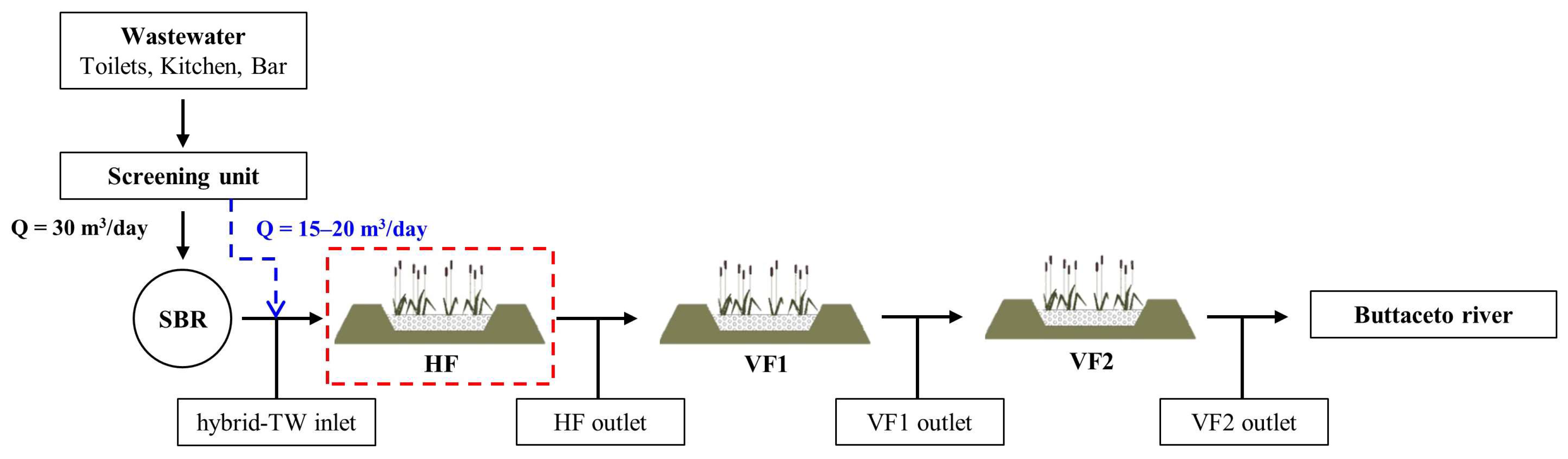
2.1. Study Area

This study was carried out in a 10-year-old HSTW used, in combination with two vertical units (V1 and V2), as a secondary WW treatment plant for the IKEA^® store situated in Catania (Eastern Sicily, South Italy, 37°26′ N; 15°01′ E) in the Mediterranean Region (Figure 1). The three units are arranged in series, with the HSTW serving as the initial stage to decrease organic matter and suspended solids (SS) concentrations. Subsequently, the two vertical subsurface TWs continue this process of reducing organic matter and SS, while also facilitating the nitrification of ammonia into nitrate. The hybrid TW was introduced in 2014 to bolster the primary sequential batch reactor (SBR) system, which has proved to be inadequate due to the pronounced fluctuations in hydraulic and organic load influent. The system was designed to treat mixed WW, receiving 30 m³ of daily effluent from the SBR and 15–20 m³ of daily effluent from the screening unit, which bypasses the SBR when the amount of WW exceeds the SBR’s design flow rate. The HSTW unit spans approximately 400 m² (12 × 34 m) with an average depth of 0.60 m. It is filled with volcanic gravel (8–12 mm) and planted with Phragmites australis at a density of 4 plants per square meter.

CR samples were collected within the HSTW in August (H1), September (H2) and October (H3) 2022 in 9 plots (each one of an area of 0.25 m²) equally distributed along 3 transects (Ts) established at 8.5 m (T1), at 17.0 m (T2) and at 25.5 (T3) m from the inlet. The biomass harvested in August was 5 months old (because the last wetland vegetation management/cutting was carried out at the beginning of March), while those harvested in September and October were about 1 month old (because they are the regrowth of August and September cuts, respectively). To determine the BMP, a subsample was prepared for each T by bulking the harvested biomass of the corresponding sample points (BT1, BT2, BT3) (Figure 2).

2.2. Common Reed Biomass Composition

Phragmites australis (Cav.) Trin ex. Steud. (common reed) is a perennial grass that belongs to the Poaceae family with a wide distribution from cold temperate regions to tropics. Thanks to its high capacity to retain various nutrients, heavy metals and micro pollutants, CR is one of the most used emergent macrophytes in the world’s wetlands. However, CR, in spite of its high above-ground dry matter yield, has been less studied for bioenergy supply compared to other energy crops. To characterize the composition of CR, measurements of fresh biomass, culm and node counts and plant heights were taken at selected harvest intervals. In particular, all the fresh biomass growth within each plot was harvested and prepared by milling using an EFCO electric shredder for chemical analysis. Then, three samples of about 100 g each were used as replicates to determine the DM content by oven drying at 65 °C until a constant weight to quantify the dry weight per culm (g DM per culm); the levels of volatile solid (VS) and ash contents were assessed following the standard procedure outlined in UNI EN 12879:2002 [25]. This involved subjecting freshly collected biomass samples to ignition at 550 °C within a muffle furnace. Hemicellulose, cellulose and lignin contents were estimated through the determination of Neutral Detergent Fiber (NDF), Acid Detergent Fiber (ADF) and Acid Detergent Lignin (ADL) using an Infrared Fiber Spectrometer. Subsamples necessary for BMP determination were created by combining the harvested biomass samples and subsequently storing them at −20 °C in accordance with the UNI/TS 11703:2018 [26] international standard.

2.3. Biochemical Methane Potential (BMP) Assay

In this study, the BMP tests played a pivotal role in evaluating methane yields from materials degraded under anaerobic conditions. The BMP determination followed the established guidelines of UNI/TS 11703:2018, which outlines a comprehensive method for assessing methane potential production via wet anaerobic digestion. This involved conducting anaerobic digestion experiments in 2 L batch reactors, with duplicate assays (D2 and D3 reactors) performed for samples harvested in August (BT1), September (BT2) and October (BT3) 2022, resulting in a total of nine tests. The addition of substrate was carefully regulated, maintaining a ratio of 2:1 between the VS of the inoculum and the substrate. To measure non-specific methane production associated with the inoculum, a control experiment (D1 reactor) was conducted using demineralized water instead of substrate. The reactors were then sealed, stored in a thermostat cabinet, flushed with oxygen-free inert gas and incubated at 37 ± 1 °C until biogas production became negligible, typically around 30 days. Throughout the BMP test duration, the biogas pressure within each reactor was continuously monitored using pressure piezo-resistive transducers.

The overall BMP value (expressed in Nm³ CH₄/tVS) was determined by averaging the BMP values obtained from each test reactor (D2 and D3).

$$BMP=\frac{\sum _1^n{BMP}_i}{n}$$

(1)

The biogas quality was assessed by measuring methane, carbon dioxide and hydrogen sulfide levels using a portable biogas analyzer (Optima7 Biogas, MRU Italia Srl, Thiene, Italy). For more details on the BMP determination procedure, see [27].

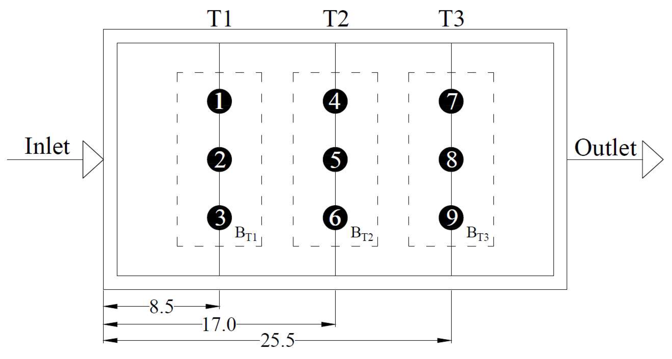
2.4. Ks Measurements

In September 2022, the falling-head method was employed to determine the Ks values within the HSTW unit. Specifically, four falling-head infiltration tests were conducted around each of the nine piezometers situated in the unit, amounting to a total of 36 measurements taken at various distances from the inlet (Figure 3). In particular, given the clogging process in the HSTW, the pervious (p) permeameter allowed us to evaluate both vertical and horizontal K_s by using Equation (2) as in [28]. The p permeameter and the corresponding equations adapted from [29] have been used since April 2018 after the calibration of the equation in [30].

$$K_s=\frac{2\pi R_{mod}+11L_{mod}}{11(t_2-t_1)}ln\left(\frac{H_1}{H_2}\right)$$

(2)

where $R_{mod}$ and $L_{mod}$ are the radius (m) and the submerged length (m), respectively, and $H_1$ and $H_2$ are the water levels (m) in the permeameter cell corresponding to time $t_1$ and $t_2$ (s), respectively. $R_{mod}$ and $L_{mod}$ are equal to 4.9 cm and 20 cm, respectively (while R and L in the original equation are equal to 5 cm and 32 cm, respectively). The interval between $t_1$ and $t_2$ is set equal to 0.25 s.

The permeameter was placed in a small hole dug in the HSTW medium until the water table was reached. Next, water was introduced into the system in a single-pulse mode using a plastic water reservoir (6.6 L volume) equipped with measurement units and a ball valve. A pressure probe (STS—Sensor Technik Sirnach, AG, Sirnach, Switzerland), connected to a laptop via a CR200-R data logger (Campbell Scientific, Logan, UT, USA), was inserted into the permeameters to monitor water level variations (H) within the measurement unit until the HSTW water table was reached. Four water level data points per second were recorded over a 30 s period. The best fit between simulated and measured water levels was determined by minimizing the squared differences between the theoretical curve and the field measurements, as expressed in Equation (3).

$${\sum }_{t=0}^n=(H_{obs}\left(t\right)-H_{sim}\left(t\right){)}^2$$

(3)

where $H_{obs}$ is the height of the water table level measured inside the permeameter at time $t$ during the test (m); $H_{sim}$ is the corresponding modelled data calculated using Equation (2). For further details on device design and the dimensions and construction of the experimental setup, see [17]. Finally, a spatial interpolation technique performed in a Geographic Information System (GIS) environment was used to assess the spatial and temporal variation in the Ks (m day⁻¹) values inside the HSTW. In detail, the inverse distance weighting (IDW) approach was applied to estimate the attribute values of an unsampled point computed as the weighted average of known values within the neighborhood assuming that the weights are inversely related to the distance between each other. This method allowed us to assign an areal significance to Ks measures recorded as point values. To perform the interpolation for one or both piezometers, the average of Ks values measured four times around each of the 9 piezometers was used. The final result was a raster image showing the Ks values variation within the HSTW.

2.5. Data Analysis

Statistix 9 software was used to conduct statistical analyses. Biomass productivity, morphological and chemical traits, methane yield of CR and Ks values were compared across HSTW transects and different harvests using one-way analysis of variance (ANOVA) to ascertain statistical significance. Upon identifying significant differences (p < 0.05), post hoc comparisons were carried out using Tukey’s honest significant difference (HSD) test at p < 0.05. Additionally, a linear regression model was employed to explore relationships among biomass characteristics, biogas yield, BMP production and hydraulic conductivity variation in the HSTW. The coefficient of determination (R2) was computed, and significance was assessed with a threshold of p < 0.05.

3. Results

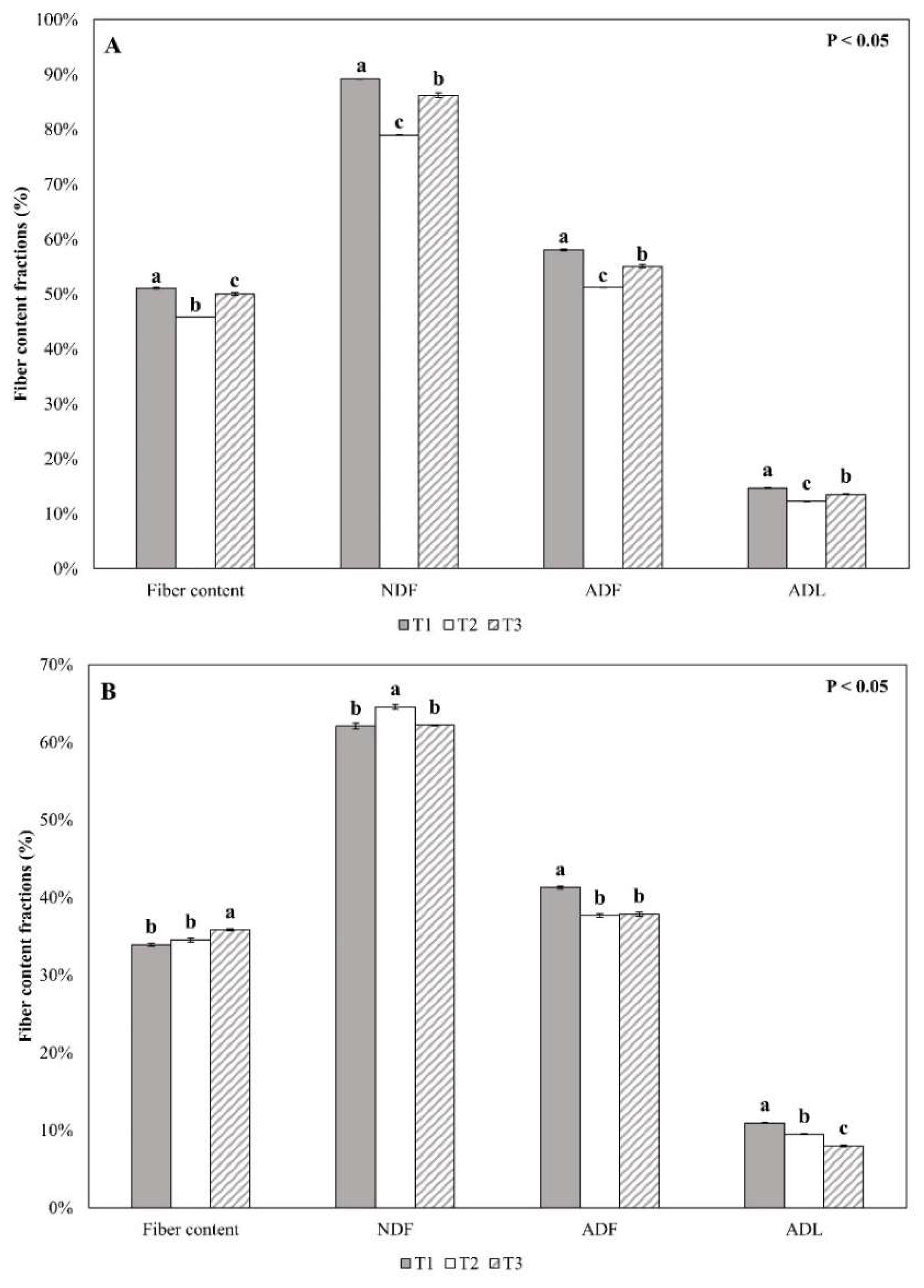
3.1. Common Reed Biomass Characteristics Variation at Different Harvest Times

The main morphological and chemical characteristics of the CRs harvested within the HSTW in H1, H2 and H3 are reported in

Table 1. Common reed morphological and chemical characteristics for different harvest times.

Properties	H1 (Aug)	H2 (Sept)	H3 (Oct)
Plant height (m) a	2.50 ± 0.05	0.78 ± 0.19	0.87 ± 0.30
Culms number (-) a	19 ± 5	25 ± 13	67 ± 26
DM (%) b	45.08 ± 0.92	22.62 ± 0.08	32.00 ± 6.38
Dry weight (g DM per culm) b	39.11 ± 8.28	4.03 ± 1.23	3.34 ± 1.10
Fiber content (%) c	48.98 ± 2.76	34.76 ± 0.97	35.21 ± 2.90
Neutral Detergent Fiber—NDF (%) c	84.75 ± 5.28	62.93 ± 1.40	63.98 ± 3.73
Acid Detergent Fiber—ADF (%) c	54.76 ± 3.41	38.94 ± 2.05	38.04 ± 4.04
Acid Detergent Lignin—ADL (%) c	13.48 ± 1.22	9.47 ± 1.49	10.32 ± 1.71

^a The data represent the mean of field measurements with their respective standard deviations. ^b The data represent the mean of three replicates with their respective standard deviations. ^c The data represent the mean of two replicates with their respective standard deviations.

.

As was expected, statistically significant differences (p < 0.05) were observed for plant height, culms number and DM content among the harvest times considering that H2 and H3 are the regrowth of the biomass harvested in summer (H1). In detail, the mean plant height ranged between 2.50 m ± 0.05 in H1 and 0.87 m ± 0.30 in H3 and the culms number surface increased during the three harvest times from a minimum of 19 ± 5 in H1 to a maximum of 67 ± 26 in H3 (Figure 4A,B). The DM content results showed significant differences (p < 0.05) among the different cuts, decreasing from H1 to H2 and H3 with plant age. In particular, the DM content ranged from a maximum of 45.08% ± 0.92 in H1 to a minimum of 22.62% ± 0.08 in H2 due to the presence of young plant tissue in September and October (Figure 4C). Also, the culms dry weight significantly decreased (p < 0.05) from H1 to H3 with plant age from older to newly formed plant tissue ranging from a maximum of 39.11 g DM ± 8.28 to a minimum of 3.34 g DM ± 1.10 (Figure 4D).

The fiber content analysis showed that significant differences (p < 0.05) occurred in the NDF, ADF and ADL content (Figure 5A–D) among the different harvest times, with higher values in the summer cut (H1) (84.75% ± 5.28, 54.76% ± 3.41, 13.48% ± 1.22, respectively) than autumn cut (H3) (63.98% ± 3.73, 38.04% ± 4.04, 10.32% ± 1.71, respectively), decreasing as the plant age decreased. There were non-significant differences in fiber fractions content between H2 and H3, which were both characterized by young tissue regrown after summer cutting. It is interesting to note that the NDF, ADF and ADL fiber fractions contents also significantly differed (p < 0.05) among the HSTW transects for each harvest time, with a heterogeneous trend showing the higher values in T1 than in T2 and T3, especially in H1 in which the plant tissues were more mature (Figure 6A). The trends in the fiber fractions contents in H2 and H3 between the HSTW transects, instead, were slightly different due to the plants’ juvenile stage (Figure 6B,C).

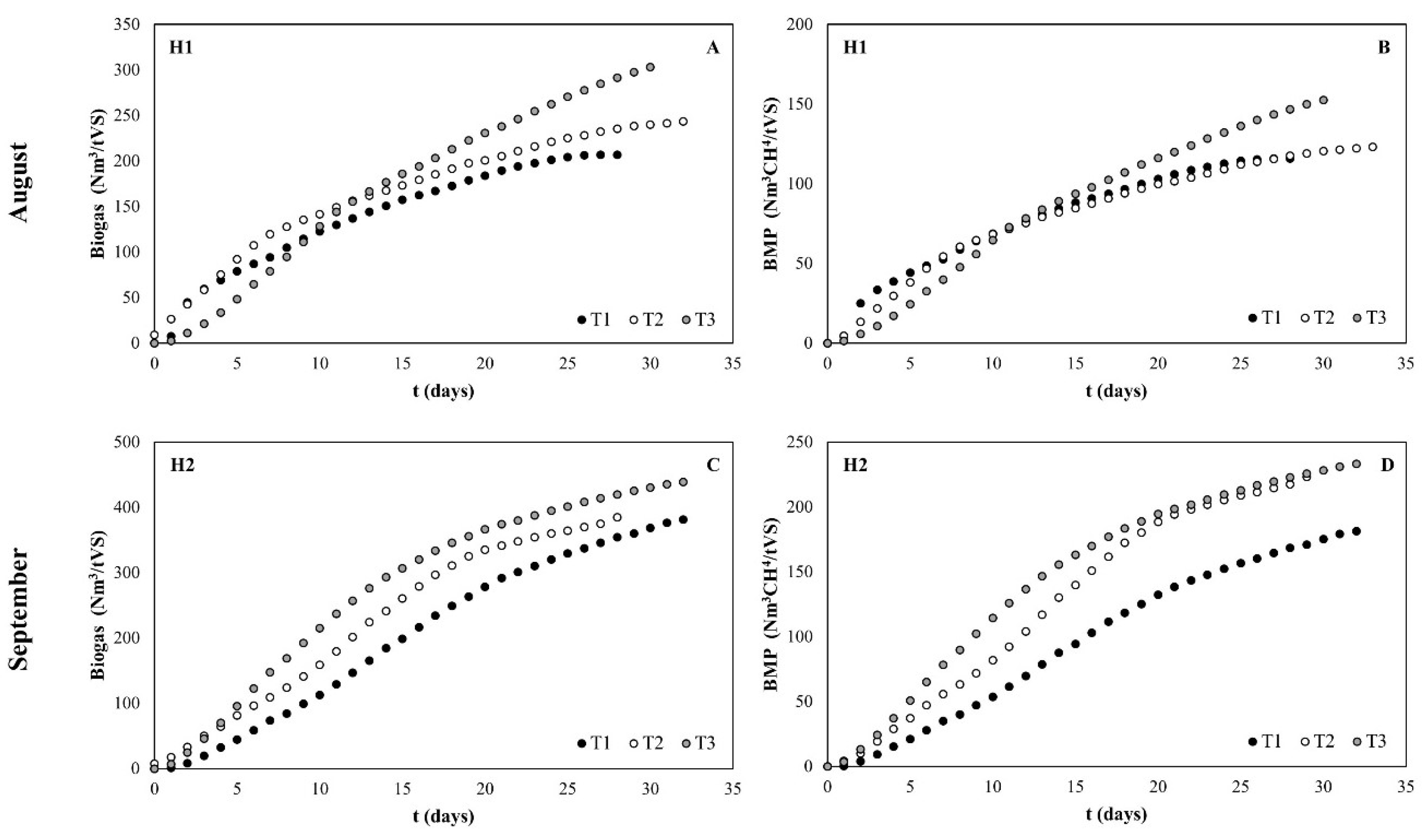
3.2. Common Reed Methane Potential Production

The laboratory tests conducted on CR samples revealed a consistent pattern in biogas and BMP production between H1 and H2, with the peak BMP value observed in September (H2) for T3 (Figure 7A). Additionally, our study’s linear regression analysis demonstrated a significant correlation (R² = 0.94) between observed biogas and BMP production trends (Figure 7B).

Table 2. BMP tests and gas quality analysis results performed on CR samples harvested in August and September 2022.

Properties	H1 (Aug)	H2 (Sept)
Biogas (Nm3/tVS) a	251.16 ± 54.72	402.08 ± 89.38
BMP (Nm3CH4/tVS) a	130.57 ± 24.29	212.70 ± 50.62
CH4 (%) a	52.32 ± 3.18	52.88 ± 5.24
CO2 (%) a	16.88 ± 4.51	14.82 ± 3.04
H2S (ppm) a	20.5 ± 14.26	74.7 ± 9.42

^a The data represent the mean of two replicates with their respective standard deviations.

summarizes the results obtained from the BMP assays and the gas quality analysis performed at lab scale. Specifically, when accounting for the two replicates (D2 and D3 reactors), the mean biogas production in H1 amounted to 251.16 Nm³/tVS ± 54.7, accompanied by a methane content of approximately 130.57 Nm³CH₄/tVS ± 24.29. (Figure 8A,B). For the H2, both the biogas production and the total amount of methane were higher than that of H1 with mean values of 402.08 Nm³/tVS ± 89.38 and 212.70 Nm³CH₄/tVS ± 50.62, respectively (Figure 8C,D). Finally, the results from the gas quality analysis performed at the end of the BMP test showed for the summer cut (H1) average contents of methane of 52.32% ± 3.18, of CO₂ of 16.88% ± 4.51 and of H₂S of 20.5 ppm ± 14.26. The H2 harvest revealed a similar trend to that of H1 showing a slightly higher methane content, with average values of 52.88% ± 5.24. The mean CO₂ and H₂S concentrations in H2 were slightly lower (14.82% ± 3.04) and higher (74.7 ppm ± 9.42) than those in H1, respectively.

Generally, the BMP production curves displayed a varied pattern for both harvests (H1 and H2), as depicted in Figure 8. The following three distinct phases of methane production emerged during the BMP test: (i) an initial delay in production commencement compared to the onset of the assay; (ii) a rapid escalation in production until reaching maximum yield, illustrated by the horizontal asymptote indicating the point at which production in the test reactors (D2 and D3) surpassed that of the blank test reactor (D1); and (iii) a gradual increase in methane production until the yield became negligible.

As shown in Figure 9, the BMP tests revealed a statistically significant difference (p < 0.05) in biogas yield and methane content between H1 and H2.

Furthermore, the DM and fiber fractions content (NDF, ADF, ADL) affected the BMP production that decreased with the increases in these parameters in the CR biomass. In our study, the linear regression analysis indicated a significant negative correlation between the observed BMP production and DM (R² = 0.50), fibers (R² = 0.51), NDF (R² = 0.51), ADF (R² = 0.59) and ADL content (R² = 0.59) (Figure 10A–C).

Regarding the outcomes derived from laboratory tests conducted on CR samples harvested in October, H3 showed the lowest biogas (mean value 201.18 Nm³/tVS ± 60.04) and biomethane yield (mean value 72.83 Nm³CH₄/tVS ± 23.19) compared to those of H1 and H2, demonstrating that the inoculum non-feed and its impoverishment over time negatively influenced BMP production which significantly decreased by, on average, 55%. The gas quality analysis also revealed lower methane contents than H1 and H2 with average values of 36.34% ± 3.97 and presented mean values of CO₂ of 7.84% ± 4.37 and H₂S of 5.5 ppm ± 6.95.

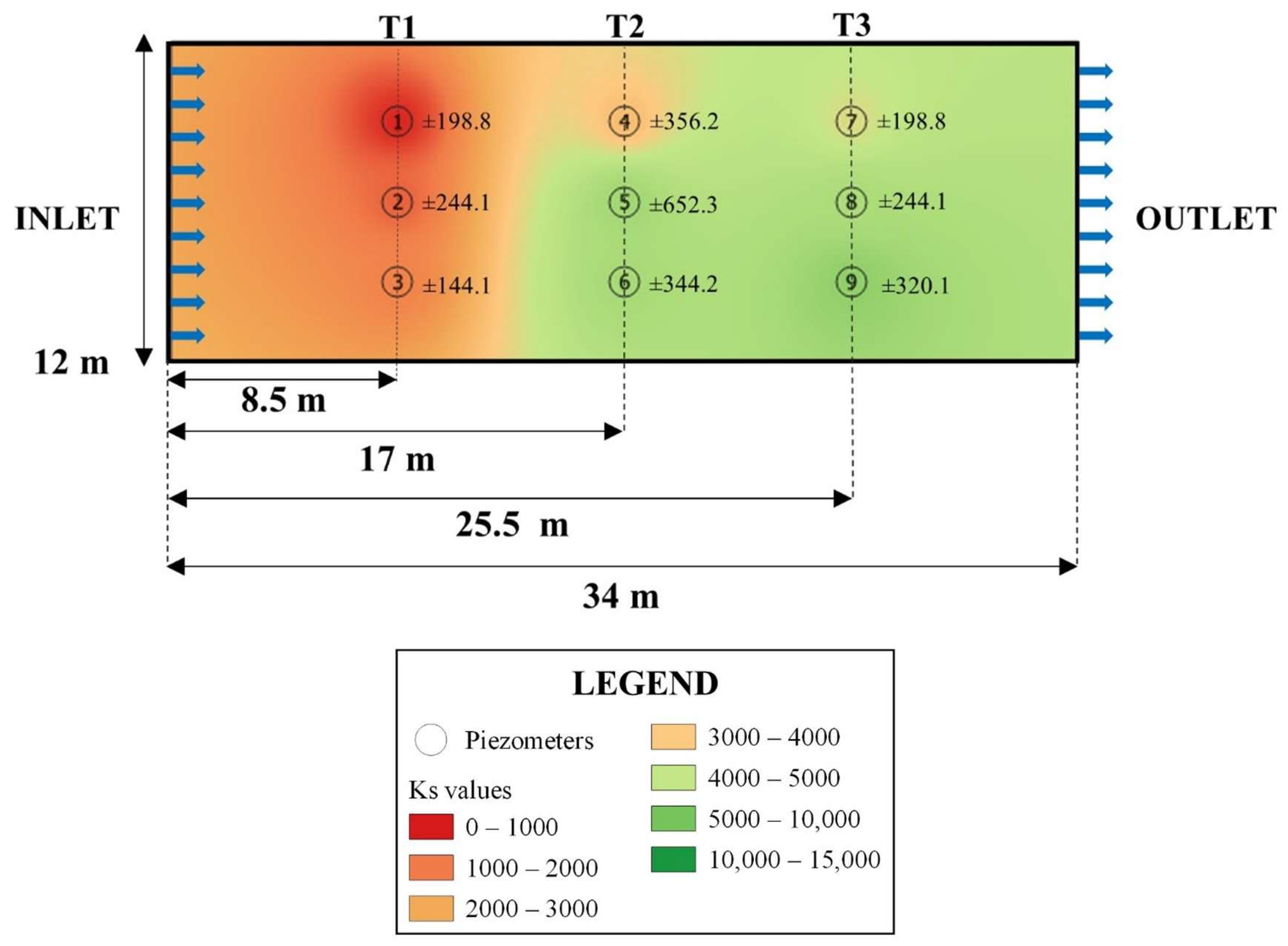
3.3. Ks Measurements within the HSTW

Table 3. Ks average ± standard deviation (SD, n = 4 per sampling point) values by each piezometer measured using falling-head method with p permeameter in the HSTW unit.

		September 2022
Piezometers	Distance from the Inlet	Ks	SD	Reductions of Ks (%)
	(m)	(m day−1)		Relative to Clean Gravel 1
1	8.5	1135.02	198.8	94
2	17	1725.13	244.1	91
3	25.5	2135.68	144.1	89
4	8.5	3568.94	356.2	82
5	17	7288.32	652.3	63
6	25.5	6895.41	344.2	65
7	8.5	4597.07	198.8	76
8	17	6570.20	244.1	66
9	25.5	8432.20	320.1	57

Note: Ks, hydraulic conductivity at saturation; SD standard deviation. ¹ Ks = 19,466 m day⁻¹.

and Figure 11 present the mean Ks values obtained using the p permeameter from each of the nine piezometers within the HSTW unit, along with their corresponding standard deviations (SD), as observed in September 2022. The Ks values recorded by piezometers 1, 2 and 3, positioned near the inlet in the T1, exhibited the lowest values, with a mean of 1665.28 m day⁻¹.

A very low Ks value was also observed for piezometer 4 of, on average, 3568.94 m day⁻¹, along the T2 (mean value 5917.56 m day⁻¹). The T3 showed the highest Ks values with a mean value of about 6533.16 m day⁻¹. Consequently, in 2022 our data showed that Ks tended to increase from the inlet to the outlet of the HSTW bed because of the high organic load that entered the hybrid-TW when the SBR system was by-passed due to the high volumes of WW produced at the IKEA^® store. Finally, the T1 results show that it was the transect that was more influenced by the clogging phenomenon.

As shown in Figure 12, the Ks measurements demonstrated a statistically significant difference (p < 0.05) in hydraulic conductivity values along the T1 and the others two transects, T2 and T3. A non-significant difference was observed between T2 and T3, which showed similar Ks values.

Furthermore, the HSTW hydraulic conductivity influenced the biomass’ morphological and chemical characteristics. Figure 13 shows clearly this phenomenon through cumulated values of culms numbers and dry weight per culm highlighting that the culms number tends to increase from T1 (which is the most clogged transect) to T3 (which is the most unclogged transect), and instead the dry weight per culm decreases from T1 to T3.

In particular, low Ks values corresponded to a greater plants’ height, but to a lower culms number. The linear regression analysis showed a strongly negative correlation between Ks values and plant height (R² = 0.85), but a significant positive correlation between Ks measures and culms number (R² = 0.56) (Figure 14A,B). As the Ks values decreased the fiber fractions content (NDF, ADF, ADL) increased as well as the DM content and the dry weight per culm, due to a large quantity of organic matter and solids in the inlet of the HSTW unit. The linear regression analysis performed in our study showed a negative correlation between Ks and fiber (R² = 0.74), NDF (R² = 0.73), ADF (R² = 0.80), ADL (R² = 0.83), DM content (R² = 0.58) and dry weight per culm (R² = 0.74) (Figure 14C–F).

Finally, considering the HSTW hydraulic conductivity’s influence on the biomass characteristics, the BMP yield also appeared to be affected, increasing as the Ks increased. In our study, the linear regression analysis indicated a slight correlation between Ks and BMP production for H1 (R² = 0.30) and a positive correlation between Ks and BMP production for H2 (R² = 0.57) (Figure 15).

4. Discussion

Our results are in line with data reported in the literature. The methane production achieved through BMP tests conducted on biomass samples collected during summer was comparable to findings from studies conducted under varied climate, plant growth and cultivation conditions. For instance, ref. [31] studied the use of summer-harvested CRs from the “Kållandsundet” drainage basin in Sweden as a raw material for biogas production, showing that they had a methane potential value of about 180 NL CH₄ kg VS⁻¹, while ref. [32] found biogas potential values varying from 400 to 500 NL CH₄ kg d.m.⁻¹ with CH₄ contents of 55–60%. In recent times, ref. [33] discussed the possibility of generating bioenergy from CR harvesting under paludiculture conditions and showed higher BMP values that decreased with crop maturity from 283 NL CH₄ kg VS⁻¹ in May to 209 NL CH₄ kg VS⁻¹ in September.

The fiber fractions content (NDF, ADF, ADL) found at crop maturity (H1) were in line with those observed by other authors [34,35]. Furthermore, according to previous findings [7,31], the results confirmed that fiber contents, especially lignin, negatively affected biomethane yield due to their recalcitrance during anaerobic digestion; for this reason, green, summer CRs (May–October) with a high nutrient content are required instead of CRs harvested in autumn that are characterized by a lower biogas potential due to their higher lignin content. In our study, younger plants harvested in September, as regrowth of the August cut, allowed us to achieve the highest biomethane production compared to the mature biomass.

Another important aspect that appeared to influence the anaerobic digestion efficiency, the BMP assay accuracy and the biomethane yield was the feeding and enriching with an inoculum made of various wastes such as agro-industrial residues, water and vegetation water prior to beginning each test. In this study, the inoculum non-feed and its impoverishment over time negatively influenced the BMP production of CR samples harvested in October, which significantly decreased by 55% on average. In recent times, ref. [27] evaluated the potential and the use of giant reeds from natural wetlands for local energy production, showing that the biomass harvest times and its characteristics affected the biomethane yield but there was no decrease in BMP production related to the inoculum that was fed and enriched prior to beginning each assay.

The evaluation of the HSTW unit’s hydraulic conductivity revealed, in line with previous studies [36,37], that the spatial evolution of clogging since the beginning of the operation period (2014) and during the observation period (2022) was more severe in the area close to the inlet along the T1 with a reduction of 91% on average for clean gravel [17,38,39]. However, to date, although related to partial clogging, numerous studies have demonstrated that there is no capacity for the reduction or removal of organic matter and suspended solids from the HSTW system and the quality of the effluent was always acceptable according to the Italian legislation limits (L.D. 152/06 and M.D. 185/03) [17,20]. Another important finding of the present study, that has not been extensively studied in previous research, is Ks’ influence on biomass growth and development, as well as on its morphological and chemical characteristics. Our results showed that, in the partially clogged areas of the HSTW, there was a lower culms number with higher dry weight per culm and height, while in the unclogged areas, the number of culms was higher, but each plant had a lower dry weight and height. In addition, the higher weight of each plant in the partially clogged area, with respect to the unclogged zone, coincided with higher fiber fractions and DM contents, due to a large quantity of organic matter and solids in the inlet of the HSTW unit, as also supported by the findings of [40] in terms of the lower COD removal efficiency observed in T1. All of this is also confirmed by the biomethane yield results obtained from the BMP assays. Consequently, the greater energy yield, in terms of methane BMP production, was obtained by using younger CR plants harvested in September within the T3, which was the most unclogged transect of the HSTW bed characterized by biomass with a low DM and fibers content.

Ultimately, our research demonstrates that TWs can be the cornerstone in the integrated management of water, nutrient and energy cycles and could contribute to the achievement of the Sustainable Development Goals (SDGs) established by the United Nation Conference on Sustainable Development (Rio +20, 2012), particularly regarding SDG Goal 6 (Ensure access to water and sanitation for all) and SDG Goal 7 (Affordable and clean energy). In addition, within the framework of the circular economy, biomass sourced from wastewater treatment plants, including crop residues, could be harnessed for energy production, thus bolstering the renewable energy cycle without encroaching on land dedicated to food production.

5. Conclusions

In this study, both the potential of TWs’ CRs’ areal biomass for biogas production and the influence of the HSTW’s hydraulic conductivity on the biomethane yield were evaluated by using a BMP testing approach. The results showed the successful possibility of integrating the depuration role of CR vegetation with the bioenergy production into TWs, thanks to the potential of CRs to produce a satisfactory methane yield despite not being a common energy crop.

Considering that the mature plant biomass (i.e., August) was characterized by a higher fiber content which negatively affected biomethane yield, younger plants (i.e., September) allowed to obtain higher BMP production. Also, the HSTW’s hydraulic conductivity appeared to influence the methane yield through plant growth and the greater energy yield was obtained by using CRs in the juvenile stages (i.e., September) harvested within the T3, which was the most unclogged transect of the HSTW bed and promoted a vegetative biomass with a low DM and fibers content.

In the framework of a circular economy, the research could contribute to encouraging plant operators to reuse biomass from TWs for local energy production in order to increase the sustainability of the system and to reduce the maintenance costs. Furthermore, this study could help plant operators (i) to understand hydraulic characteristics’ effects on biomass development and on its chemical and morphological characteristics, and (ii) to improve TWs treatment efficiency, system management and lifespan. Therefore, vegetation within wastewater treatment plants could significantly contribute to bioenergy production while also serving as a crucial component of the wastewater treatment process. This supplementary role of biomass could facilitate the expansion of wastewater treatment plants in inland Mediterranean Regions, where larger surface areas are available compared to coastal areas.

References

1. Vymazal, J. Emergent plants used in free water surface constructed wetlands: A review. Ecol. Eng. 2013, 61, 582–592. [Google Scholar] [CrossRef]
2. Avellan, C.T.; Ardakanian, R.; Gremillion, P. The role of constructed wetlands for biomass production within the water-soil-waste nexus. Water Sci. Technol. 2017, 75, 2237–2245. [Google Scholar] [CrossRef] [PubMed]
3. Licata, M.; Gennaro, M.C.; Tuttolomondo, T.; Leto, C.; La Bella, S. Research focusing on plant performance in constructed wetlands and agronomic application of treated wastewater—A set of experimental studies in Sicily (Italy). PLoS ONE 2019, 14, e0219445. [Google Scholar] [CrossRef] [PubMed]
4. Meng, P.; Hu, W.; Pei, H.; Hou, Q.; Ji, Y. Effect of different plant species on nutrient removal and rhizospheric microorganisms distribution in horizontal-flow constructed wetlands. Environ. Technol. 2014, 35, 808–816. [Google Scholar] [CrossRef] [PubMed]
5. Zhang, D.Q.; Jinadasa, K.; Gersberg, R.M.; Liu, Y.; Ng, W.J.; Tan, S.K. Application of constructed wetlands for wastewater treatment in developing countries—A review of recent developments (2000–2013). J. Environ. Manag. 2014, 141, 116–131. [Google Scholar] [CrossRef]
6. Liu, D.; Wu, X.; Chang, J.; Gu, B.; Min, Y.; Ge, Y.; Shi, Y.; Xue, H.; Peng, C.; Wu, J. Constructed wetlands as biofuel production systems. Nat. Clim. Chang. 2012, 2, 190–194. [Google Scholar] [CrossRef]
7. Köbbing, J.F.; Thevs, N.; Zerbe, S. The utilisation of reed (Phragmites australis): A review. Mires Peat 2013, 13, 1–14. [Google Scholar]
8. Geurts, J.J.; Oehmke, C.; Lambertini, C.; Eller, F.; Sorrell, B.K.; Mandiola, S.R.; Grootjans, A.P.; Brix, H.; Wichtmann, W.; Lamers, L.P.; et al. Nutrient removal potential and biomass production by Phragmites australis and Typha latifolia on European rewetted peat and mineral soils. Sci. Total. Environ. 2020, 747, 141102. [Google Scholar] [CrossRef] [PubMed]
9. Dandikas, V.; Heuwinkel, H.; Lichti, F.; Drewes, J.E.; Koch, K. Correlation between Biogas Yield and Chemical Composition of Grassland Plant Species. Energy Fuels 2015, 29, 7221–7229. [Google Scholar] [CrossRef]
10. Kandel, T.P.; Sutaryo, S.; Møller, H.B.; Jørgensen, U.; Lærke, P.E. Chemical composition and methane yield of reed canary grass as influenced by harvesting time and harvest frequency. Bioresour. Technol. 2013, 130, 659–666. [Google Scholar] [CrossRef]
11. Ragaglini, G.; Dragoni, F.; Simone, M.; Bonari, E. Suitability of giant reed (Arundo donax L.) for anaerobic digestion: Effect of harvest time and frequency on the biomethane yield potential. Bioresour. Technol. 2014, 152, 107–115. [Google Scholar] [CrossRef] [PubMed]
12. Dragoni, F.; Ragaglini, G.; Corneli, E.; o Di Nasso, N.N.; Tozzini, C.; Cattani, S.; Bonari, E. Giant reed (Arundo donax L.) for biogas production: Land use saving and nitrogen utilisation efficiency compared with arable crops. Ital. J. Agron. 2015, 10, 192–201. [Google Scholar] [CrossRef]
13. Yang, Z.; Wang, Q.; Zhang, J.; Xie, H.; Feng, S. Effect of plant harvesting on the performance of constructed wetlands during summer. Water 2016, 8, 24. [Google Scholar] [CrossRef]
14. Wang, Q.; Xie, H.; Zhang, J.; Liang, S.; Ngo, H.H.; Guo, W.; Liu, C.; Zhao, C.; Li, H. Effect of plant harvesting on the performance of constructed wetlands during winter: Radial oxygen loss and microbial characteristics. Environ. Sci. Pollut. Res. 2015, 22, 7476–7484. [Google Scholar] [CrossRef] [PubMed]
15. Al-Isawi, R.; Scholz, M.; Wang, Y.; Sani, A. Clogging of vertical-flow constructed wetlands treating urban wastewater contaminated with a diesel spill. Environ. Sci. Pollut. Res. 2015, 22, 12779–12803. [Google Scholar] [CrossRef] [PubMed]
16. Knowles, P.; Dotro, G.; Nivala, J.; García, J. Clogging in subsurface-flow treatment wetlands: Occurrence and contributing factors. Ecol. Eng. 2011, 37, 99–112. [Google Scholar] [CrossRef]
17. Licciardello, F.; Sacco, A.; Barbagallo, S.; Ventura, D.; Cirelli, G.L. Evaluation of different methods to assess the hydraulic behavior in horizontal treatment wetlands. Water 2020, 12, 2286. [Google Scholar] [CrossRef]
18. de Matos, M.P.; von Sperling, M.; de Matos, A.T. Clogging in horizontal subsurface flow constructed wetlands: Influencing factors, research methods and remediation techniques. Rev. Environ. Sci. Bio/Technol. 2018, 17, 87–107. [Google Scholar] [CrossRef]
19. Tang, Y.; Yao, X.; Chen, Y.; Zhou, Y.; Zhu, D.Z.; Zhang, Y.; Zhang, T.; Peng, Y. Experiment research on physical clogging mechanism in the porousmedia and its impact on permeability. Granul. Matter 2020, 22, 37. [Google Scholar] [CrossRef]
20. Vymazal, J. Does clogging affect long-term removal of organics and suspended solids in gravel-based horizontal subsurface flow constructed wetlands? Chem. Eng. J. 2018, 331, 663–674. [Google Scholar] [CrossRef]
21. Sanford, W.E.; Steenhuis, T.S.; Parlange, J.-Y.; Surface, J.M.; Peverly, J.H. Hydraulic conductivity of gravel and sand as substrates in rock-reed filters. Ecol. Eng. 1995, 4, 321–336. [Google Scholar] [CrossRef]
22. Suliman, F.; French, H.; Haugen, L.; Søvik, A. Change in flow and transport patterns in horizontal subsurface flow constructed wetlands as a result of biological growth. Ecol. Eng. 2006, 27, 124–133. [Google Scholar] [CrossRef]
23. Pedescoll, A.; Uggetti, E.; Llorens, E.; Granés, F.; García, D.; García, J. Practical method based on saturated hydraulic conductivity used to assess clogging in subsurface flow constructed wetlands. Ecol. Eng. 2009, 35, 1216–1224. [Google Scholar] [CrossRef]
24. Garcia-Artigas, R.; Himi, M.; Revil, A.; Urruela, A.; Lovera, R.; Sendrós, A.; Casas, A.; Rivero, L. Time-domain induced polarization as a tool to image clogging in treatment wetlands. Sci. Total Environ. 2020, 724, 138189. [Google Scholar] [CrossRef]
25. UNI EN 12879:2002; Characterization of Sludges—Determination of the Loss on Ignition of Dry Mass. UNI: Rome, Italy, 2002.
26. UNI/TS 11703:2018; Method for the Measurement of the Potential Production of Methane from Wet Anaerobic Digestion—Matrices in Feed. UNI: Rome, Italy, 2018.
27. Sciuto, L.; Licciardello, F.; Barbera, A.; Cirelli, G. Giant reed from wetlands as a potential resource for biomethane production. Ecol. Eng. 2023, 190, 106947. [Google Scholar] [CrossRef]
28. Naval Facilities Engineering Command. Soil Mechanics. Design Manual 7.01; Nav. Facil. Eng. Command: Alexandria, VA, USA, 1986. [Google Scholar]
29. Pedescoll, A.; Samsó, R.; Romero, E.; Puigagut, J.; García, J. Reliability, repeatability and accuracy of the falling head method for hydraulic conductivity measurements under laboratory conditions. Ecol. Eng. 2011, 37, 754–757. [Google Scholar] [CrossRef]
30. Licciardello, F.; Aiello, R.; Alagna, V.; Iovino, M.; Ventura, D.; Cirelli, G.L. Assessment of clogging in constructed wetlands by saturated hydraulic conductivity measurements. Water Sci. Technol. 2019, 79, 314–322. [Google Scholar] [CrossRef] [PubMed]
31. Hansson, P.-A.; Fredriksson, H. Use of summer harvested common reed (Phragmites australis) as nutrient source for organic crop production in Sweden. Agric. Ecosyst. Environ. 2004, 102, 365–375. [Google Scholar] [CrossRef]
32. Komulainen, M.; Simi, P.; Hagelberg, E.; Ikonen, I.; Lyytinen, S. Reed Energy—Possibilities of Using the Common Reed for Energy Generation in Southern Finland. Rep. Turku Univ. Appl. Sci. 2008, 67, 81. [Google Scholar]
33. Dragoni, F.; Giannini, V.; Ragaglini, G.; Bonari, E.; Silvestri, N. Effect of Harvest Time and Frequency on Biomass Quality and Biomethane Potential of Common Reed (Phragmites australis) Under Paludiculture Conditions. BioEnergy Res. 2017, 10, 1066–1078. [Google Scholar] [CrossRef]
34. Dinka, M.; Ágoston-Szabó, E.; Tóth, I. Changes in nutrient and fibre content of decomposing Phragmites australis litter. Int. Rev. Hydrobiol. 2004, 89, 519–535. [Google Scholar] [CrossRef]
35. Wohler-Geske, A.; Moschner, C.R.; Gellerich, A.; Militz, H.; Greef, J.M.; Hartung, E. Provenances and properties of thatching reed (Phragmites australis). Landbauforsch 2016, 66, 1–10. [Google Scholar] [CrossRef]
36. Xu, Q.; Chen, S.; Huang, Z.; Cui, L.; Wang, X. Evaluation of organic matter removal efficiency and microbial enzyme activity in vertical-flow constructed wetland systems. Environments 2016, 3, 26. [Google Scholar] [CrossRef]
37. Vymazal, J. Removal of BOD in constructed wetlands with horizontal sub-surface flow: Czech experience. Water Sci. Technol. 1999, 40, 133–138. [Google Scholar] [CrossRef]
38. Knowles, P.; Davies, P. A method for the in-situ determination of the hydraulic conductivity of gravels as used in constructed wetlands for wastewater treatment. Desalination Water Treat. 2009, 5, 257–266. [Google Scholar] [CrossRef]
39. Pedescoll, A.; Knowles, P.R.; Davies, P.; García, J.; Puigagut, J. A comparison of in situ constant and falling head permeameter tests to assess the distribution of clogging within horizontal subsurface flow constructed wetlands. Water Air Soil Pollut. 2012, 223, 2263–2275. [Google Scholar] [CrossRef]
40. Sacco, A.; Sciuto, L.; Licciardello, F.; Cirelli, G.L.; Milani, M.; Barbera, A.C. Effects of Solids Accumulation on Greenhouse Gas Emissions, Substrate, Plant Growth and Performance of a Mediterranean Horizontal Flow Treatment Wetland. Environments 2023, 10, 30. [Google Scholar] [CrossRef]
Figure 1. Design of the hybrid-TW system at the IKEA® store in Catania (Eastern Sicily, South Italy). Red frame indicates the HSTW unit, which is the subject of this study.
Sustainability 16 02751 g001
Figure 2. HSTW experimental unit. Black dots are above-ground biomass sampling plots.
Sustainability 16 02751 g002
Figure 3. Setup of the HSTW bed showing the locations of piezometers and saturated hydraulic conductivity (Ks) measurements.
Sustainability 16 02751 g003
Figure 4. Common reed morphological and chemical characteristics according to different harvest times (H1–H3). (A) Plant height; (B) culms number; (C) dry matter content; and (D) dry weight per culm. Different letters indicate statistically significant differences (p < 0.05).
Sustainability 16 02751 g004
Figure 5. Common reed fiber fractions content according to different harvest times (H1–H3). (A) fiber content; (B) Neutral Detergent Fiber (NDF) content; (C) Acid Detergent Fiber (ADF) content; and (D) Acid Detergent Lignin (ADL) content. Different letters indicate statistically significant differences (p < 0.05).
Sustainability 16 02751 g005
Figure 6. Common reed fiber fractions content according to different HSTW transects (T1–T3). (A) August; (B) September; (C) October. Different letters indicate statistically significant differences (p < 0.05).
Sustainability 16 02751 g006aSustainability 16 02751 g006b
Figure 7. (A) Curves of biogas and BMP production. The values are the means of the different HSTW transects for each harvest time (August—H1 and September—H2). (B) Relationship between observed biogas and BMP production.
Sustainability 16 02751 g007
Figure 8. Curves of biogas and BMP production performed for each HSTW transect (T1–T3) of the CR samples harvested in August (H1) and September (H2). (A) Biogas yield in August; (B) BMP production in August; (C) biogas yield in September; (D) BMP production in September.
Sustainability 16 02751 g008
Figure 9. Biogas and BMP production according to different harvest times (August—H1; September—H2). Different letters indicate statistically significant differences (p < 0.05).
Sustainability 16 02751 g009
Figure 10. Relationship between observed BMP production and (A) DM, (B) fibers, (C) NDF, ADF and ADL content.
Sustainability 16 02751 g010
Figure 11. Spatial variation of Ks (m day−1) values for the 9 piezometers inside the HSTW bed in September 2022 obtained by using the inverse distance weighting (IDW) approach in a Geographic Information System (GIS) environment.
Sustainability 16 02751 g011
Figure 12. Ks values according to different HSTW transects (T1–T3). Different letters indicate statistically significant differences (p < 0.05).
Sustainability 16 02751 g012
Figure 13. Cumulated values of culms number and dry weight per culm according to different HSTW transects (T1–T3).
Sustainability 16 02751 g013
Figure 14. Relationship between measured Ks values and (A) culms number, (B) plant height, (C) DM content, (D) dry weight per culm, (E) fiber content, (F) NDF, ADF and ADL content.
Sustainability 16 02751 g014
Figure 15. Relationship between measured Ks values and BMP production.
Sustainability 16 02751 g015