Vision-Based Reinforcement Learning Approach to Optimize Bucket Elevator Process for Solid Waste Utilization

Abstract

An energy-intensive industry such as cement manufacturing requires a constant supply of high amounts of traditional fossil fuels, such as coal or gas, for the calcination process. A way to overcome this fuel need is the usage of solid waste or Alternative Fuel Resources (AFRs), such as wood or paper. An advantage of using such waste is that their combustion byproduct, “ash”, can be used as a raw material alternative in the cement manufacturing process. However, for structural reasons, only bucket elevator technology is feasible to convey the fuel vertically for feeding the calciner in most cement plants. During the fuel feeding process, the inhomogeneous characteristics of AFRs lead to discharge parabolas of these materials varying over the infeed sample. Hence, a need arises to observe these trajectories and estimate a method for their optimal discharge. Thus, the purpose of this study is to develop an intelligent high-performance bucket elevator system. As such, a vision-based reinforcement learning algorithm is proposed in this study to monitor and control the speed of the elevator depending on the material properties observed at the inlet. These inlet materials properties include the type of material used in the simulation, and the particle size distribution within the infeed sample. A relationship is established between the inlet material properties and the speed of the bucket elevator. The best possible scenario is then deduced using a reward function. Here, the reward function is formulated via the deep learning image segmentation algorithm, a novel approach. After observing the test simulation conducted with a random-parameters setup, it was noted that the optimum speed for a given infeed sample was predicted correctly. As such, it can be concluded that the goal of developing an intelligent bucket elevator system was achieved.

1. Introduction

A large amount of energy is required for thermal production across manufacturing industries. In particular, the cement industry requires thermal heat production through the calcination process. Traditionally, coal is used as fuel to feed the calciner in cement plants. A calciner is a steel cylinder located within a furnace. With a controlled atmosphere, it performs indirect high-temperature raw fuel processing (550–1150 °C) by rotating inside a heated furnace. This fuel is usually dumped in the furnace at an elevated height using bucket elevator technology. An example of such a system can be seen in Figure 1. For structural reasons, bucket elevator technology is the only viable vertical conveying option for feeding the calciner with fuel in most cement plants. With sustainability and resource conservation, there is an increasing trend towards the substitution of classical fossil fuels, such as coal or gas, by Alternative Fuel Resources (AFRs) across the process industry [1]. Some of these fuel particles that have been considered include materials such as wood straws, rubber granules, paper waste, wood chips, etc.

The solid waste or AFRs have calorific values that are sufficient to generate the heat needed for the calcination process. Also, high temperatures in the calciner facilitate the complete combustion of these waste products, which minimizes the chances of harmful emissions. The combustion of AFRs results in a byproduct in the form of residual ash. This ash has transformative potential in the cement manufacturing process, as discussed in [2]. The ash exhibits pozzolanic properties. The durable cement compounds are formed when lime is combined with pozzolan materials. Here, the ash byproduct can be used as an alternative raw material for cement manufacturing. The ash could also replace clinker, another raw material for cement manufacturing, thereby contributing to a significant reduction in CO2 emissions.

The usage of AFRs for cement production at the stage of the cement combustion process has been explored in [3]. It provided a detailed study of actively monitoring a multi-fuel burner using traditional image analysis concepts for the use of AFRs dynamically in energy production. However, the problem of optimizing an AFR material infeed for such a burner remained an open question. Biomass or waste streams are the primary sources to procure these AFRs. And, as such, they possess inhomogeneous bulk material characteristics, such as humidity, density, and particle size distribution. Although the usage of such materials is environmentally favorable, conventional bucket elevators are not suitable, with the often fluffy and inhomogeneous substitute fuels, to efficiently feed these materials in heat furnaces. The inhomogeneous characteristics of AFRs lead to discharge parabolas of these materials varying over the sample that is discharged. Hence, a need arises to observe these trajectories and estimate a method for their optimal discharge. This article, therefore, aims to develop an intelligent high-performance bucket elevator. The idea is to optimize the speed of the bucket elevator intelligently. A reinforcement learning (RL) algorithm controlled by a vision-based reward function is proposed to achieve this goal. However, training an RL algorithm requires a large amount of quality data. Acquiring high-quality data in large volumes with an actual bucket elevator requires operating the machine multiple times, which is a cumbersome process that leads to high energy consumption along with potential wear and tear on the system. An alternative approach is to collect data from a simulation that replicates the behavior of the system and transfer the learning from the virtual experience to the real world. As such, the research is carried out by optimizing the bucket elevator simulation based on the software coupling of Computational Fluid Dynamics (CFD) and the discrete element method (DEM). The ability to numerically calculate finite element particle displacements and rotations and to automatically perform contact detection for a group of different particle types is called the discrete element method [4]. The DEM uses Newton’s laws of motion and numerical integration for background computation purposes. As such, the software is capable of calculating forces acting on particles and, thus, acceleration, velocity, and position for every particle. With a discretized approach behind the DEM, the method is well suited for modeling the bulk materials’ behavior. Based on the simulation models, discharge parabolas, and online measurement data, intelligent control of the conveying process is developed.

In order to illustrate the volatility of typical AFRs, Figure 2 provides an overview of different fuel types typically used as a heat source, e.g., within the cement clinkering process. As is immediately visible from their visual appearance, their general bulk material properties (e.g., humidity, particle size distribution, bulk density, etc.) vary enormously. Furthermore, even the same types of fuel (e.g., wood chips) tend to have inhomogeneous characteristics, since they are mostly produced by different fuel preparation plants and, therefore, originate from different source material streams. It can be stated, in general, that all of the shown fuels have non-supporting characteristics when it comes to their transportation within a bucket elevator. Most of the fuels tend to be quite coarse, lumpy, and fibrous, and have a relatively low bulk density, if compared to homogenous bulk materials, such as sand or cement.

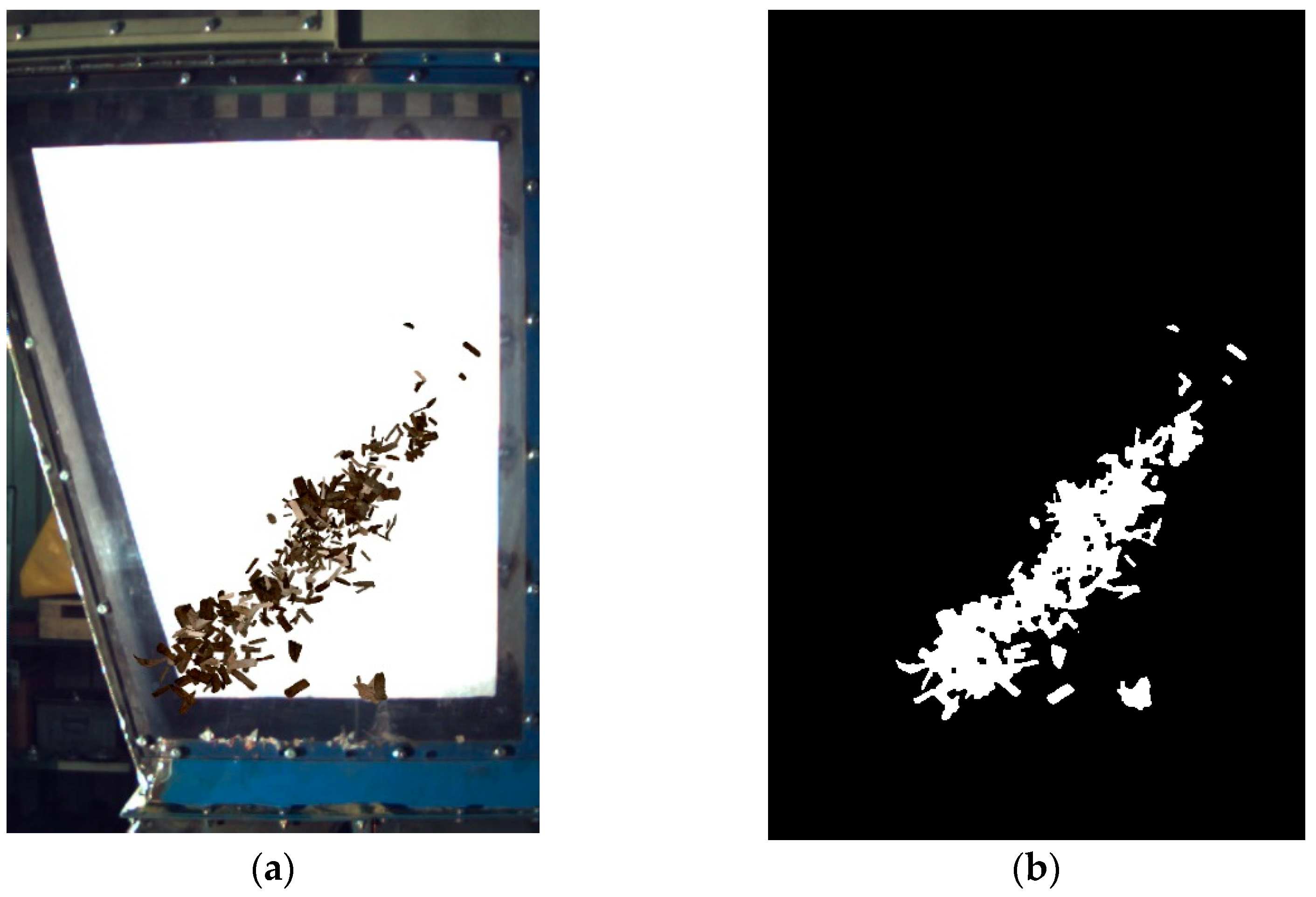
To increase the efficiency of the bucket elevator, it is important to analyze the discharge trajectory of the material and control it. The idea is to ensure that the maximum amount of material gets disposed into the target furnace rather than back into the elevator base. General studies about the discharge behavior of bucket elevators have been carried out for decades, which led to a general theoretical model of bucket elevator discharge trajectories (see [5]). However, most of the work considers only homogenous bulk materials or the actual mechanical design of the machine itself (see [6]).

A particular work about inhomogeneous AFRs was done by Rammrath in his thesis (see [7]). In [7], a proof of concept was established with respect to calculating the discharge parabolas of these AFRs. The work focused on using tools of the OpenCV (Open Source Computer Vision) library such as morphological operation, canny edge detection, and the RANSAC (Random Sample Consensus) algorithm to estimate the trajectories of AFRs. However, the study was limited to the detection of the external edge of discharge material due to approach implementation restrictions. After computing the theoretical-based discharge parabola representation using Müller’s Theoretical Drop Model, the study concluded that a balancing function needs to be developed to estimate the exact dependence of a discharge parabola on various material properties of AFR particles. The typical properties that define the material behavior are Young’s modulus, the Poisson ratio, the coefficient of friction, the coefficient of restitution, the coefficient of rolling friction, and cohesion. As discussed earlier, the process would be conducted in a CFDEM-based experimental simulation setup. Much research has been done to simulate the exact behavior of bulk materials in DEM simulations. Namely, two common approaches are followed, microscopic and macroscopic approaches to calibrate DEM material parameters. The microscopic approach analyzes the direct contact-level information such as density and the coefficient of friction between particles to simulate bulk materials. On the other hand, the macroscopic approach observes the overall behavior of DEM simulation compared to real work values. A broad application of these approaches to determine and calibrate DEM parameters is available in [8,9]. One of the prime studies that piqued our interest was our co-author Elbel’s thesis work where he uses the RL algorithm to estimate the bulk material properties. The concept behind Elbel’s work was to use an Advantage Actor–Critic (A2C) RL algorithm to replicate two targets’ static and dynamic angles of repose in a DEM simulation close to the real-world value. The angle of repose is the measure of the flowability of bulk material and is located between the horizontal plane and the material surface. To achieve this objective, various combinations of four different bulk material properties were tried out in a systematic manner. This idea was also one of the motivations behind the current research.

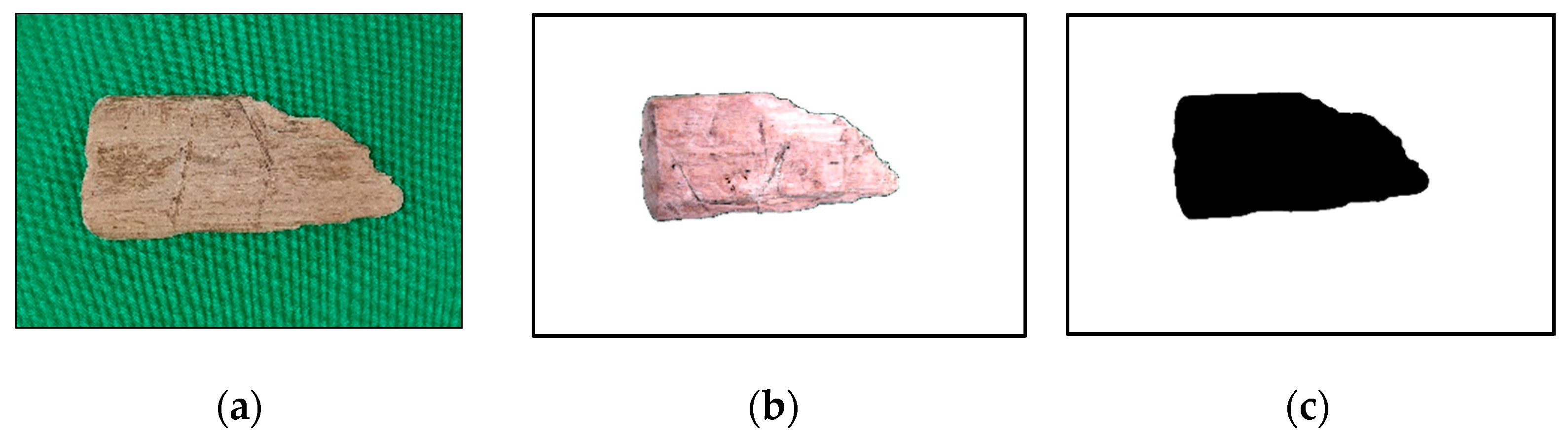
Optimizing the material discharge parabola requires understanding and correlating various physical properties of materials such as density, particle size distribution (PSD), and flowability. One such work implemented preceding this article was the online PSD estimation based on a DL-based segmentation approach, a detail of which is available in [10]. This work would also have a significant role in describing the state of the RL system agent. A notable outcome of this work was the use of a synthetically generated image dataset for the segmentation task. The alpha channel of the individual particle images was manipulated to form the superset of images. As the reward function of the RL agent used in this research is based on a combination of computer vision (CV) and the DL concept, a modified version of the synthetic dataset generation algorithm described in [10] was used to achieve the task of dataset formation. The important objective of that article was to detect the region within an image where the particles were present at a given time. Such a task is referred to as an image segmentation task. During the last decade, researchers have developed a plethora of convolutional-based models for image segmentation. It all started when the image segmentation task became highly efficient with the successful segmentation of biomedical images for brain tumor detection using the deep learning architecture UNET described in article [11]. The UNET architecture is based on convolutional operators that extract important local features of the image. However, they are still limited in modeling a global context, and this is where a more advanced transformer-based UNET architecture took over. A notable application of these vision transformers can be seen in article [12]. That paper provides a thorough comparison of vision transformers with different segmentation model variants for a forest fire image segmentation task and ascertains their improved performance compared to more traditional UNET architecture. A similar variant of the vision transformer is also used in this work.

The training or learning of an algorithm based on its interactions with a dynamic environment is the ML branch called reinforcement learning. The reinforcement learning algorithm consists of an agent or a brain that continuously observes the state of the environment and interacts with it to change it to a required or optimized state by performing an action. It can be said to be a trial-and-error process of learning over time. The measure of how good or bad is the action taken by an agent is the reward. The aim is to maximize the reward. One key aspect of RL is the need to find the trade-off between exploration and exploitation of the environment. With the aim to maximize the reward, the agent could get stuck in local minima where the probability of getting a good reward is high. However, there could be another region in the state space where a much better reward can be obtained, and the agent should keep exploring for the same. Hence, the agent must decide whether to take the risk of exploration in an effort to find better rewards or to exploit the current experience of the environment [13]. This problem scenario of exploration vs. 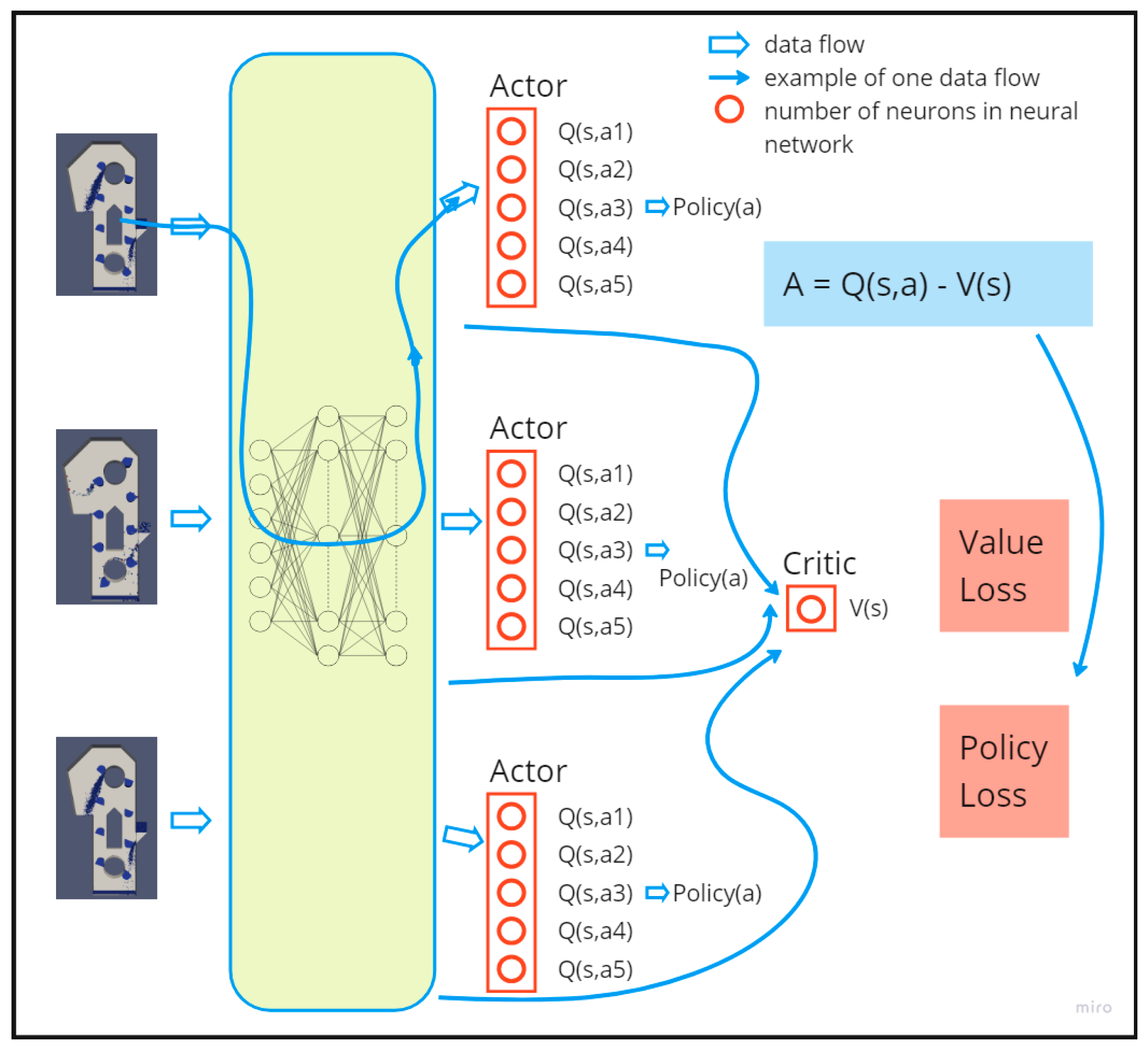exploitation of the environment, as stated by Sutton, one of the founding members of the RL field, is still in the research stage, and is mostly resolved based on the domain knowledge of RL application [13]. One of the advanced RL algorithms that minimizes the scenario of exploration vs. exploitation is the Asynchronous Advantage Actor–Critic (A3C) algorithm. It enables the agent to explore unique states and at the same time work on the known one. A variant of such an A3C algorithm is used in this work, and the choice of considering such an algorithm is further discussed in the later subsection.

To summarize, this article provides a short overview of the proposed framework in Section 2. It also consists of discussions of two important parts of the methodology, namely CV and a DL-based approach for detecting discharge parabolas and the optimization of bucket elevator throughput using RL. This is then followed by evaluating the approach to different scenarios in Section 3. The algorithm for detecting the material discharge parabola and, thereby, the RL reward function will be evaluated. And, this will be followed by the test of the RL algorithm in a test simulation setup. The paper is finalized with a conclusion and discussion of future scope.

2. Methodology

This article focuses on the online optimization of the bucket elevator discharge process using the tools of Artificial Intelligence. An overview of this unique approach is elaborated in this section and can be visualized in Figure 3.

As seen in Figure 3, the RL’s environment is the bucket elevator simulation itself. To optimize the process, the bucket elevator was constantly monitored. The monitored parameters included the type of the infeed material, the particle size distribution of the infeed material, the infeed rate of the material, the velocity of the bucket elevator movement, and the average mass of the material within a bucket and at the outlet of the elevator. Of these mentioned parameters, the type of the infeed material, the particle size distribution, the infeed rate of the material, and the velocity of the bucket elevator were used to describe the state of the environment. Based on the current state values, the agent processed them and produced an action in the form of a change in bucket velocity magnitude. The action brought a change to the environment, which in this case was the change in the discharge trajectory of the material. This change was measured in terms of a segmented image percentage value of the desired area. This was accomplished using a combination of computer vision and a deep learning algorithm. As such, it produced a continuous value in the range of 0 to 1, which acted as a reward signal for the RL algorithm. Based on this, the bucket elevator achieved an optimum speed of discharge for a given set of material properties. A detailed step-by-step implementation of each aspect of the process is explained in subsequent stages.

2.1. CV and DL-Based Approach for Detection of Discharge Trajectory of AFR Material

In this study, a combination of CV and a DL-based approach was used to track the discharge behavior of AFR material. However, to implement this approach in reality, a large chunk of well-labelled material trajectory data was needed. To conduct such activity on site with an actual bucket elevator system is a challenging task accompanied by a huge electric power requirement. As such, a novel approach using discrete element method (DEM) simulation software called LIGGGHTS (version 3.7.0) has been proposed in this study. With an aim to improve the production process and solve industrial problems, LIGGGHTS is used to simulate particle behavior in the fields of chemical, pharmaceutical, agricultural, and food production, mining, and many more [14]. This DEM simulation used a spring-damper contact model explained in [15] to compute the simulation stats.

The functioning of the bucket elevator with AFR material was simulated and the data from LIGGGHTS software were extracted. Here, the data were extracted in terms of the centroid coordinates of the individual particles within the simulation. These data were processed and used to generate the dataset containing images and corresponding masks. Finally, a deep learning algorithm for an image segmentation task was used to determine the parabola behavior at the outlet of the bucket elevator. As stated in article [16] by Minaee et al., deep learning-based segmentation models can be classified into 10 different categories based on the model architecture. In this study, two variants of an encoder–decoder-based model were used and are explained in the next subsections.

2.1.1. Discrete Element Simulation-Based Experimental Setup

The simulated experimental setup consists of LIGGGHTS input scripts that when executed generate Visualization Toolkit (VTK) files. However, an important aspect of the usage of LIGGGHTS software is its interface capabilities with the Python language. LIGGGHTS enables certain methods such as extract_atom(), get_atoms(), extract_variable(), etc. that allow the user to transfer the computed data of LIGGGHTS into Python for further processing. The prime data that were accessed from LIGGGHTS were the number of particles in the simulation at any given time, their corresponding coordinates within the system, and the differentiating factor (radius or density) of each corresponding particle. To conduct the next task of dataset generation, the resulting particle coordinates needed to be normalized. Also, it is important to load the normalized coordinates along with the corresponding radius simultaneously. As such, these activities were conducted using Python as the backbone. An example of a VTK file-based setup visualized using Paraview software (version 5.6.1) is shown in Figure 4.

2.1.2. Synthetic Dataset Generation

For a deep learning-based model to detect the discharge parabolas, a well-labelled dataset is essential. A labelled dataset refers to an exact correspondence between a set of images and the underlying particle contours, also called ground truth images. This process, if conducted manually, could lead to a higher probability of human errors. As such, a novel concept for synthetic dataset generation used in [10] was adapted to achieve this task.

• Background Separation

As implemented in [10], about 500 individual wood particle images of varying shapes and sizes were captured. An industrial camera with an image resolution of 1024 × 768 pixels was used for this purpose. Here, firstly the individual particle region of interest was extracted by converting the image background to black in HSV (Hue Saturation Value) format followed by the “bitwise_and” logical operation. This was followed by changing the region of interest’s alpha channel to opaque and the rest to transparent. A sample of such alpha channel-manipulated images can be seen in Figure 5. At the same time, a mask was extracted for the corresponding particle images by using OpenCV library tools, mainly binary thresholding and morphological. A detailed guide about the process can be found in [10]. The improvised procedure of [10] used for the study objective is formally presented in Algorithm 1.

Algorithm 1 Background separation of individual particles and their contour generation

procedure bg_separation(images)  for the particle in images do    Detect the background by inspecting its pixel range    Extract the particle using bitwise “and”    Create a copy of the extracted particle      Convert the original extracted image to grayscale followed by a blur    Pass the image to the inverse binary thresholding technique to obtain the mask    Apply morphological transformations    Get the sure foreground area using the distance transformation method    Manipulate the alpha channel of particle contour using the sure foreground area      Manipulate the alpha channel of the extracted particle using the sure foreground    area    return extracted particle and its contour end procedure

• Image and Mask creation

The design of the bucket elevator used in a real-world scenario is such that only the area marked red in Figure 4 is a Plexiglass surface. Any analysis that can be done via vision sensor techniques is limited to that region. Hence, only those particle coordinates in the simulation that belong in the Plexiglass region were considered for image generation and, hence, for parabola detection. The coordinates extracted have the values in the simulation range domain. Hence, they were first normalized in the range of image pixel resolution. The normalized coordinates of simulated particles extracted from LIGGGHTS were used as centroids for placing the background-separated particles. At the same time, the mask extracted for the corresponding particle images was placed simultaneously at the same location. Before placing the particles at the respective coordinates, the radius information of the given particle was used to resize the particle image with respect to real-world sizes. The overlapping importance between the particles was taken care of by the alpha channel-based manipulation, a detailed guide about which can be found in [10]. The adapted procedure of [10] used for the study objective is formally presented in Algorithm 2. Once the alpha channel-manipulated particle images and corresponding masks are placed at the respective locations, one can easily obtain an infinite amount of overall parabola images at any given time. A sample of such images and ground truths (masks) can be seen in Figure 6. Thus, the dataset was ready, with training and testing images and respective masks, to use for training in a segmentation model. The standard ratio of an 80/20 split for train and test sets, respectively, was maintained.

Algorithm 2 Image and mask generation

procedure generation(manipulated_images, canvas, centroids, radii)   for index in the length of centroids do     if radii[index] in the list of radii do       Resize the manipulated_images[index] to appropriate resolution       Normalize alpha channel of both canvas and manipulated_images [index]       Over-relay manipulated_images [index] on canvas using array mutation   return canvas end procedure

2.1.3. UNET Deep Learning Model

The UNET architecture is a deep learning-based model used for contour or semantic segmentation tasks. It consists of two parts, namely contracting and expansive, as seen in Figure 7. The contracting part, composed of downsampling blocks, extracts a high-dimensional feature map of input images by using the concept of convolutional layers. The downsampling blocks consist of a pair of 3 × 3 convolutional layers, a batch normalization layer, and an activation function in the form of a rectified linear activation function, or ReLu. This is followed by max pooling of kernel size 2 × 2, which highlights import features within feature maps. The expansive part composed of upsampling blocks decodes the feature and predicts the mask of the objects. The upsampling block contains a deconvolutional layer that halves the feature channels. Then, the result is concatenated with the corresponding downsampling block’s feature channels, also called skip connections. This is, again, then followed by a pair of 3 × 3 convolutional layers, a batch normalization layer, and a ReLu. The employed architecture was composed of four downsampling and four upsampling blocks. Finally, a 1 × 1 convolutional layer produced the mask of the input, which in this case was the detected discharge parabola. The success of UNET is mainly contributed by the presence of skip connections. These skip connections provide the upsampling block with low-level texture information, which is a crucial factor in the generation of high-level semantic feature outputs. The detected discharge parabola still had some irregularities in segmented output. These were mostly observed at the edges of the segmented parabola. Thus, to provide the ML algorithm with this global context, another model was trained and evaluated from the domain of vision transformers. Detailed information about its architecture is explained in the next section.

2.1.4. TransUNET Deep Learning Model

TransUNET is a hybrid CNN–transformer model, which, consistent with the previous UNET architecture, is also a U-shaped model integrating both the transformer and UNET network, as illustrated in Figure 8. It combines the advantage of UNET (high resolution of local features extracted by a CNN) and the transformer (encoded global contextual information by attention mechanism) to generate a powerful segmentation model. Similar to UNET, the architecture of TransUNET can be divided into two parts, namely, the encoding or contracting part followed by the decoding or expansive part. The encoding part contains three downsampling blocks composed of CNNs that extract key features. A part of these extracted feature maps was used in the corresponding upsampling block as skip connections. Furthermore, the output of the final downsampling block was tokenized into a 2D embedding or patch embedding by means of linear projection. The embedding encoded positional information. This was followed by the attention mechanism of the transformers. The employed architecture contained eight transformer layers. Here, each layer, as illustrated on the left side of Figure 8, contained a normalization layer, a Multi-Layer Perceptron (MLP), and a Multi-Head Self-Attention (MSA) mechanism. An MLP comprises several fully connected layers. The MSA mechanism was the main driving block behind the transformer usage and was based on the dot product attention mechanism, inspired by the work of Vaswani et al. in [17]. Finally, to enable the input of the decoding part of the transformer, the output was reshaped to the required value. In the expansive part, the reshaped output feature maps were passed through upsampling blocks in a manner similar to the UNET process. As such, the architecture employed four upsampling blocks. Lastly, a 1 × 1 convolutional layer produced the mask of the input, which in this case was the detected discharge parabola. A better segmentation result was obtained using TransUNET, which will be discussed later.

2.1.5. DL-Based Image Segmentation Algorithm

As DL segmentation models require high computational power to train, a 24 GB GPU (Graphical Processing Unit) was utilized, with training conducted under the framework of the deep learning library PyTorch. Initially, the images were resized to a lower resolution of 496 × 320 pixels to ease the computation burden. A few image pre-processing techniques were employed to enhance the features of images. It is important to ensure that there is a smooth transition between particles and background within an image. Also, the edges must be preserved. To ensure that this requirement was met, a median filter was used for image pre-processing. This was followed by normalizing the image pixel values between 0 and 1. The pre-processing techniques employed for both UNET and TransUNET were the same.

The pre-processed images were then loaded randomly in batches to ensure the generalization of data within a batch while training. The training was conducted with an optimizer function in the form of Adam, and a scheduled learning rate with a fixed starting learning rate value was considered. The binary cross entropy was used as a loss function as the predicted model output and the ground truth had binarized pixel values to compare.

The grad scaler, an Automatic Mixed Precision technique in PyTorch, was used during the gradient calculation. The model and optimizer parameters of the data type tensor are usually in float32 type. The grad scaler converts them to float16 type for calculations, which in turn increases the training speed and reduces the VRAM memory usage. A summarized specification regarding the various parameters used for training purposes in both cases can be found in

Table 1. DL Training specifications.

Model	UNET	TransUNET
Resolution	496 × 320	496 × 320
Training Images	3380	3380
Testing Images	820	820
Batch Size	8	8
Epochs	30	68
Learning Rate	1 × 10−3	1 × 10−4
Optimizer	Adam	Adam
Loss Function	BCE	BCE
Trainable Parameters	31,037,633	149,820,143

.

2.2. Optimization of Discharge Parabolas of Infeed Materials in DEM Simulation Using RL

The DEM simulation of spheres works as an environment that is combined with a reinforcement learning (RL) algorithm to optimize the trajectory. The process is divided to form a two-step approach. This includes a training phase, in which the RL agent learns the specific behavior of the material and relationships between the different system parameters. Afterward, the pre-trained agent uses the DEM simulation to optimize the discharge material trajectory for any given system state. To validate the results, for a given set of system parameters, the average material mass at the inlet for an individual bucket is calculated and compared with the average mass of material dumped by an individual bucket at the outlet. This reveals the success status of the optimization approach.

2.2.1. RL Environment Setup

The environment is an overall action space where in which an agent works to change the current state of the system. For a given state of a system, the environment receives an action signal that generates a reward/penalty based on how good/bad is the new state that the environment ends in. In this study, the LIGGGHTS input scripts were used as an RL environment in which we changed certain parameters at regular instances. These parameters basically defined the state of the system at a given time. An example of a LIGGGHTS simulation-based system environment can be seen in Section 2.1.1. Within this setup, two distinct types of behavior of the system were developed. The two simulation system behaviors can be approximately considered the behavior of paper and wood particles in a real bucket elevator system and, as such, will be called by these aliases in this work. A simulated visualization of these can be seen in Figure 9.

As the optimization process was managed by the change in the speed of the bucket elevator, particular care must be taken while working with the data extracted from the simulation. The change in the speed of the elevator brought a change in the amount of material filled within the bucket at that time. Thus, a dynamic waiting time must be incorporated for the corresponding bucket elevator speed. This was to ensure that the current time matched the time at which the bucket reached the data extraction point, i.e., the top of the bucket elevator. Afterward, the data were extracted for a set of five buckets to have a mean value of material flow at a given speed of the elevator.

2.2.2. State Space of RL

In the optimization of the bucket elevator process, we defined the state of the system by four important parameters, namely, the speed of the elevator, the type of material used in the simulation, the rate of infeed of material, and the particle size distribution within a particular infeed material sample shown in Figure 10. In a simulation, these state values can be easily extracted from the LIGGGHTS script at a given time. In a real-world bucket elevator system, the speed of the bucket elevator and the infeed rate of material can be obtained via their respective Variable–Frequency drives. The information regarding the type of material at the inlet along with the particle size distribution within a sample can be procured using a deep learning-based segmentation approach, discussed in [10].

Depending on the state of the system, the RL agent has a choice to increase or decrease the speed of the elevator by a certain predefined magnitude. As this action brings a change in the system state, the algorithm calculates the magnitude of the change. This is called a reward. This reward defines whether the agent performed an optimum action or not. The process of assigning rewards will be explained further in the next stage.

2.2.3. Action Space of RL

The optimization process was carried out by manipulating the bucket elevator velocity. The operating velocity of the system was established in a range between 0.5 m/s and 2.0 m/s. With the goal of obtaining an optimum velocity of the bucket for a given state of the system, the velocity was found by converting the operating velocity range into a discretized space. Hence, certain magnitude jumps were established and assigned to each action. Thus, in total, 5 actions were available to the agent to perform. Of these, 4 actions were of different magnitude and direction, and an additional action was formulated to repeat the same velocity. This additional action ensured that the agent would perform the same action (no change of velocity) once it had reached the optimum velocity value.

2.2.4. Reward Function

In simple terms, a reward is a positive or negative feedback that an agent receives in return for its interaction with the environment. In the current case study, a unique approach is proposed in relation to the reward function. Here, the segmented discharge parabola obtained from the process discussed in Section 2.1 is considered a reward decision window. It can be seen in Figure 8 that the discharge parabola has many outliers that are not necessarily important with respect to trajectory tracking. Hence, these outliers were first removed. A density-based clustering mechanism called DBScan was employed here. It is an unsupervised machine learning algorithm that identifies clusters in datasets by observing the local density of the data points [18]. A minimum radius parameter in the form of an epsilon needs to be fixed, which decides what set of data points form a cluster. After an analysis based on the K-distance graph, the epsilon value was chosen to be 30. As such, the outliers were removed and we proceeded to the next stage of reward function formulation.

At this point, all the white pixels (detected parabola) population was calculated within an image window. However, from the optimization perspective, the main goal is to minimize the event of discharge of AFR material back to the elevator base. As such, to increase the magnitude of the surveillance on this particular area, a relatively smaller window of the complete detected discharge parabola section was considered for reward calculations. A visualization of this reward window can be seen in Figure 11. Within this reward window, a red marked area, as shown in Figure 11, was established whereby any particle present within this area would end up back within the elevator bottom surface. The size of this area was based on observed and analyzed particle discharge trajectories and, thus, is a hyper-parameter that can be further tuned to improve the algorithm efficiency. Thus, we calculated the percentage of material (white pixels) that would be outside this unwanted elevator region (red-marked). The result of such a hypothesis is a continuous reward value that drives the agent to reach an optimal stage. In order to verify the functionality of this hypothesis, a few test setups were developed, which are discussed in Appendix A.

To push the agent quickly out of the unwanted region in case of extreme scenarios (e.g., when a major chunk of material is flowing back to the bucket elevator base), a bigger penalty was added to the existing reward function. This penalty was applied based on a threshold value of the segmentation output. In this case, the penalty was applied if the area of particles present in the red region was greater than 30%. Another important phenomenon that was observed during the trajectory analysis was that a greater amount of material was transported at the outlet if the bucket elevator was running at lower speed values. Thus, the goal should be to find the optimum discharge behavior of the bucket elevator at the lowest possible speed. To incorporate this information into the reward calculations, a certain magnitude of the current speed of the bucket was subtracted from the existing reward value. The magnitude of this speed factor was considered drastically lesser than the magnitude of the segmentation-based reward, as the main goal was to first find the optimum speed. Thus, the overall reward can be summarized as seen in Equation (1).

$$R=\left\{\begin{array}{c}if 100-se{g}_{percent}>30\%\\ x,\hspace{1em}\hspace{1em}-2+\underset{0}{\overset{se{g}_{percent}}{\int }}dx\\ .\\ else\\ x,\hspace{1em}\hspace{1em}-1+0.9\ast \underset{0}{\overset{se{g}_{percent}}{\int }}dx+0.1\ast (1-Norm\left(v\right))\\ .\\ 2,\hspace{1em}\hspace{1em}if m_o\ge 0.95\ast m_i\\ .\end{array}\right.$$

(1)

Here, R is the reward, $m_o$ is the mass of material at the outlet bucket, $m_i$ is the mass of material at the inlet bucket, $se{g}_{percent}$ is the percentage of segmentation material at the outlet as indicated earlier, Norm indicates a normalized value, and $v$ is the velocity of the bucket elevator.

2.2.5. Asynchronous Advantage Actor–Critic (A3C) Algorithm

One of the major hindrances that arose with the use of DEM simulation as an RL environment was that the Python interface only enabled the usage of one processing core at a time. This drastically reduced the complete usage of available computing power. This is where the Asynchronous Advantage Actor–Critic (A3C) algorithm used in [19] proved to be beneficial. Here, the term asynchronous indicates the usage of unique environment instances running parallelly. This makes the overall experience available for training more diverse, as each environment state change is independent of others. Thus, with each core running a distinct simulation-based environment, there is a possibility to have somewhere around 8 to 10 environments running in parallel to train the agent of the A3C algorithm. The training takes place based on the outputs received from any environment as they arrive, i.e., online training on a first-arrived, first-used basis. This approach can be visualized using Figure 12.

An actor–critic algorithm, as the name suggests, involves exploring two outputs. An actor in the algorithm is responsible for estimating the policy function [π(s)], which indicates the optimal policy to use. The critic is responsible for estimating the value function [V(s)], which indicates the value for being in the current state. Thus, an actor performs an action by following a policy, and the critic’s aim is to criticize these actions. The performed action by an actor can be described mathematically as

$$Q\left(s,a\right)=r+\gamma V\left(s^{\prime }\right)$$

(2)

where Q(s, a) is the action value for the current state “s”. “r” is the reward for the action performed, $\gamma$ is the discount factor, and $V\left(s^{\prime }\right)$ is the value of the previous state $s^{\prime }$. At any given time, an advantage signal is computed by the critic based on its value, which can be expressed as,

$$A\left(s,a\right)=Q\left(s,a\right)-V\left(s\right)$$

(3)

$$A\left(s,a\right)=r+\gamma V\left(s^{\prime }\right)-V\left(s\right)$$

(4)

where A(s, a) is the advantage signal. This advantage has the responsibility of adjusting both the policy and value function by backpropagating the error in the network. Here, a positive advantage indicates that the current state value is better than expected, and a negative advantage means the state value is worse. The optimization of both policy and value is done simultaneously. By having the same neural network for both the policy and value function, the network learns much faster and more effectively. It can be said that the actor improves performance, and the critic makes the model more precise.

2.2.6. Deep Feed Forward Neural Network (DNN)-Based RL Agent

The state space of the system describes the actual state of the RL environment at a given time. In the current work, these states are discrete numerical values. Based on these values, the agent computes the probabilities of every possible action along with a value describing how good the chosen action is using the highest probability. As such, these numerical calculations can be performed by means of a DNN network. A DNN is a kind of artificial neural network but contains more than one hidden layers, hence the term “deep”. The DNN network architecture used for this task can be visualized in Figure 12. The agent is defined here by means of the PyTorch neural network module. It consists of a common base (state space and hidden layers), an actor (action space), and a critic (value function neuron).

As seen in Figure 13, the number of the input neurons of the brain is decided by that of the state space, which is six. The number of output neurons is decided by that of the action space, in this case, five. The network consists of two hidden layers with thirty-two neurons each. In between these two hidden layers, an activation function, ReLu, is used. It filters out all the negative values generated from hidden layer one and, thus, encourages the agent to add non-linearity into the process. Finally, a softmax function is used at the output of the network, i.e., the action space, to generate probabilities for action space. As explained in the A3C algorithm section, the action space forms the actor, and the additional neuron at the end forms the critic. Both parts of the A3C algorithm branch out from a common base of hidden neurons. And, the error is propagated by the weighted sum of these two parts while training the algorithm.

2.2.7. RL Training Parameters for Optimization of Discharge Parabolas

A well-defined RL environment based on the LIGGGHTS spherical particle type was established. The next stage was to define the various parameters needed for the overall agent training, which can be found in

Table 2. RL Training specifications.

Parameters	Values
Number of processes (environments)	10
Number of episodes in each process	22
Maximum steps in each episode	25
Learning rate	1 × 10−3
Discount factor	0.99
Hidden layers	2
Hidden neurons/layer	32
Optimizer	Adam
Particle radii	3, 1.5, and 0.5 cm

. The values of these parameters are based on the authors’ understanding of the system and also on the computational restrictions. The values were finalized from the test setup experience and produced good optimization results, which will be discussed in the result evaluation section.

As seen in Table 2, ten independent DEM simulations were running simultaneously for training, with each simulation using one core of processors. This enabled us to make fully optimal use of the available resources to train the agent for the optimization task. An important factor to note is that in the training phase, the input state space values were normalized in the range of 0–1 before being passed on to the agent. This ensured that the agent gave importance to all values in input features of a similar scale or extent. This, in turn, improved the performance and training stability of the agent during activities such as gradient descent.

3. Result Evaluation and Testing

In the evaluation of the material discharge segmentation algorithm, real-world bucket elevator images conveying wood pellets were used. The performance of both UNET and TransUNET DL models was evaluated on these wood pellet images. The three evaluation metrics, namely, dice score/F1 score, IoU score/Jaccard Index, and Segmentation Precision, were used for performance measurement. Here, a dice score coefficient can be defined as the value of the overlap area between two images divided by the total number of pixels in both images [20]. In simple terms, it indicates the measure of similarity between two images. An IoU can be defined as the value of the overlap area between the segmentation prediction and the ground truth divided by the area of union between the two images. An IoU of 1 indicates exactly identical images and a best score. The way IoU is defined leads to penalizing single instances of bad classification more than the dice score. Thus, the IoU is always quantitatively less than the dice score. The Segmentation Precision (SA) metric used in [11] was also employed for the performance evaluation.

During the evaluation of the RL algorithm, a random set of material parameters used in state space was considered along with the random starting point of the elevator velocity. The RL algorithm was then run in evaluation mode. In this mode, only those actions with the highest probability in the action space were performed. The system was analyzed to check if the bucket elevator reached an optimum speed for a given set of material parameters. The optimum speed in this scenario was the point at which 95% of the material conveyed in a bucket at a given time would be discharged at the outlet. With the framework as explained in the Methodology section developed, this section will first evaluate the DL-based discharge segmentation algorithm followed by testing and evaluating the actual bucket elevator optimization approach.

3.1. DL Algorithm Evaluation for Discharge Material Segmentation

This section provides the evaluation of the two DL models discussed earlier. The resulting evaluations are first done on the synthetic images, which the models were never trained on. This is then followed by the evaluation comparison using the real-world bucket elevator images in the consequent subsection.

3.1.1. UNET Evaluation

With the training parameters indicated in Table 1, a decrease in the value of the loss function over the epochs was noticed. It is important to note that the decreasing pattern was similar for both the training and testing datasets’ losses. This indicates the model parameters were not over-fitted to the training dataset but, rather, the model learned a generalized representation of the notable features within the images. These features are the spatial information, such as a change in textures and colors, that distinguishes the material from the background surface. The decreasing pattern of the training loss function over the epochs can be visualized in Figure 14.

To ascertain the loss theory, it was found that the UNET model algorithm was able to achieve a dice score of 0.9725 for the test dataset. The plot for the dice score evaluation over the training epochs can be seen in Figure 15. An increasing trend in the dice score was observed, which shows improved performance as the training progressed. An early stop function was implemented based on the test dice score value in the program. This function incorporates a counter that waits up to a predefined threshold (in the study, a value of 10) for an increase in the dice score value. Once this threshold passes, the model stops its training. A better visual understanding regarding the prediction of the UNET model can be obtained by observing some random sample images chosen from the synthetic test dataset.

3.1.2. TransUNET Evaluation

The TransUNET model was also trained with the parameters indicated in Table 1. The resultant DL model was able to segment the test dataset with a slightly better dice score value of 0.9736. The corresponding training loss also displayed a decreasing loss over the epochs. A graph of the same behavior can be seen in Figure 16. However, it took more training time than UNET to achieve the best dice score. One of the prime reasons for this is the usage of a comparatively smaller learning rate (1 × 10⁻⁴). With a higher value of learning rate, the problem of exploding gradients was observed. Also, with a higher number of trainable parameters present in the model, the problem of exploding gradients was magnified. To avoid this scenario, a gradient clipping mechanism was implemented that limits the values of the gradient update to a certain threshold. This process of clipping or clamping the gradient prevents the model parameters from having a huge update during backpropagation and, thus, avoids the degeneration of the algorithm.

The plot for the dice score evaluation over the training epochs in the case of the TransUNET model can be seen in Figure 17. Similar to the UNET model, an increasing trend in the dice score was observed, which shows improved performance as the training progressed. Also, an early stop function implemented in UNET was incorporated here with a threshold value of 10. During this period, the test dice score of an active epoch was checked with the previous one for improvement. Once this threshold passed, the model stopped its training.

A better visual understanding regarding the prediction of the TransUNET model can be obtained by observing some sample images chosen randomly from the synthetic test dataset. Two of such unique sample images’ predictions are drawn out in Figure 18. Also, a brief comparison of the performance metrics of two DL models on the test dataset can be found in

Table 3. DL Evaluation results.

Metric	UNET	TransUNET
Dice Score	0.9725	0.9736
Segmentation Precision	0.9723	0.9723
IoU Score	0.9644	0.9665

.

3.1.3. Algorithm Evaluation Using Real-World Images

It is necessary that the proposed approach works for real-world image segmentation. An evaluation was conducted on a few of the captured bucket elevator images. Two such image predictions can be visualized in Figure 19.

It can be seen that the proposed approaches are able to segment the trajectory up to a certain extent. However, there are also some false segmentations present within the predicted image. The reason could be the lower quality of the captured images. The camera used for this task was an industrial camera with an image resolution of 0.4 MP. Fine-tuning the model prediction by training with a better-quality background image could help to overcome these false segmentations within the predicted images.

Although the performance of TransUNET was slightly better compared to UNET, more computation resources were required to achieve this performance. This is due to the four-fold greater trainable parameters present in TransUNET compared to UNET, as indicated in Table 1. Hence, when choosing the right model for the trajectory segmentation, a comprise must be made based on required performance and computational power availability.

3.2. RL Optimization Process Evaluation

With the masked images readily available at this instance for the reward calculation, the training and testing process of the RL agent was initiated. The various parameters and hyper-parameters used in this process are described in Table 2. The evaluation of the RL optimization process can be divided into two phases. The first phase involves training the RL agent so that it can correlate its network parameters to different states that are observed within the system. In this training phase, an advantage function, described in Section 2.2.5., was backpropagated through the agent to learn this correlation function. A detailed performance description regarding the learning phase of the agent is explained in the first subsection. This is followed by testing the learned behavior in the second phase or test phase. This helped us to evaluate the performance of the proposed approach in the bucket elevator process optimization.

3.2.1. RL Training Phase

With the higher computation cost behind the usage of DEM simulation, the RL training algorithm went on for 20 days. The training was conducted in such a way as to ensure that 95% of the material within a bucket at the inlet was transferred to the outlet for optimum discharge. During this period, a total of 220 episodes, each consisting of a varying number of unique steps ranging between 2 and 25, were carried out. Some promising results were obtained after this training duration.

Figure 20 shows the earned reward during the training procedure. The abscissa represents the total number of performed training steps, whereas the ordinate describes the possible reward range. As seen in the graph, at least until 3300 steps, most of the RL agent’s earned reward is on the negative side of the graph. This indicates that the RL agent was still learning the system’s behavior. However, as it approached 3500 steps, there was an increase in the occurrence of maximum reward of +2. This indicates that most of the agent’s actions at this interval led to the system reaching the required optimal state.

A better performance indication of the algorithm’s behavior can be obtained by observing the loss function plot. The overall loss function behavior over the episodes is visualized in Figure 21.

The overall training loss is a combination of policy and value loss. Thus, the behavior of the overall loss is influenced by the values of policy and value loss, and their visualization is provided in Figure 22. In these graphs, the blue-colored distribution indicates the loss values, and a mean over 10 episodes was calculated and is represented in orange. It can be noticed from these graphs that the loss values displayed highly oscillating behavior in the initial phase, i.e., until 180 episodes. As the training progressed, these oscillations were reduced, and the mean value shows a steady movement towards the zero-loss value. This means the RL policy was adjusting towards mapping the right actions from a given state. This is possible because of the advantage function, using which the critic was able to predict the best expected reward. When the loss function reached close to a zero value, the training process was stopped, and the learned parameters were stored.

3.2.2. RL Testing Phase—System Evaluation

The testing phase used the trained agent to control the bucket elevator simulation. At any given instance, the system described by the state space was analyzed by the pre-trained RL agent. This analysis resulted in a decision that brought a change in the magnitude of the bucket elevator speed. The quality of how good or bad this decision was was then measured in the backend by the DL-based reward function. Based on the trained RL agent, a few test scenarios were conducted to check if the randomly initiated state of the bucket elevator DEM simulation was able to reach the optimum velocity. Two such test scenarios, one each for the wood and paper simulations, will be illustrated further.

In the case of a test wood simulation scenario, a visualization of the various parameter changes over the steps can be observed in Figure 23. The initial state of the system in this scenario consisted of an elevator velocity of 1.8 m/s, a constant material infeed rate of 0.5 m/s, and a PSD within the infeed material sample consisting of 21% of 3 cm, 17% of 1.5 cm, and 62% of 0.5 cm radii spheres. The figure shows that three parameters of the setup were tracked over the step progress. These parameters were the material mass/bucket at both the inlet and outlet, and the change in velocity over the steps. A better visualization of this test scenario can be observed in Figure 24. In here, the impact of the given velocity on the material discharge can be seen. During the RL-based optimization process, a few snapshots at discrete intervals were captured and are presented. It can be seen that at the elevator speed of 1.55 m/s, most of the material within the discharge parabola belonged to the unwanted region (red area) of the reward window (green) discussed in Section 2.2.4. This led to a higher negative reward value. But as the agent progressed towards decreasing the bucket elevator velocity in the wood case, more and more material was driven out of this unwanted red region and towards the outlet, which led to a better reward. The RL agent then stopped the optimization process once almost 95% of material mass within a bucket measured at the inlet was discharged at the outlet section, which in this particular scenario was at the 1.05 m/s bucket elevator velocity.

Another scenario, of the paper setup DEM simulation, was tested. The initial state of the system in this scenario consisted of an elevator velocity of 1.0 m/s, a constant material infeed rate of 0.5 m/s, and a PSD within the infeed material sample consisting of 43% of 3 cm, 5% of 1.5 cm, and 52% of 0.5 cm radii spheres. The plot for this setup can be observed in Figure 25.

A better visualization of this test scenario can be seen in Figure 26. There, the impact of the given velocity on the material discharge can be seen. During the RL-based optimization process, a few snapshots at discrete intervals were captured and are presented. It can be seen that at the elevator speed of 1.1 m/s, most of the material within the discharge parabola belonged to the unwanted region (red area) of the reward window (green) discussed in Section 2.2.4. This led to a higher negative reward value. But as we progressed towards increasing the bucket elevator velocity (a trend that the RL agent learned during training, in particular for paper-type particles), more and more material was driven out of this unwanted red region and towards the outlet section, which led to a better reward. It can be noticed that the agent was able to move the elevator velocity towards the optimal value, where 95% of the material within a bucket at the inlet was transferred at the outlet (see

Table 4. RL testing parameters.

		Case 1 (Wood)	Case 2 (Paper)
PSD (3 cm, 1.5 cm, and 0.5 cm radii spheres)		21, 17, and 62%	43, 5, and 52%
Initial elevator velocity		1.8 m/s	1.0 m/s
Final elevator velocity		1.05 m/s	1.5 m/s
Material—mass/bucket	Inlet	$2.9301\mathrm{k}\mathrm{g}/{\mathrm{m}}^3$	$1.4779\mathrm{k}\mathrm{g}/{\mathrm{m}}^3$
	Outlet	$2.7993\mathrm{k}\mathrm{g}/{\mathrm{m}}^3$	$1.4750\mathrm{k}\mathrm{g}/{\mathrm{m}}^3$

). The velocity in this case was found to be 1.5 m/s. Once the agent reached this stage, the DEM simulation episode stopped further exploration. A brief overview of the various parameters involved in both cases can be found in Table 4.

4. Conclusions

The objective of this study is to make a provision for the utilization of Alternative Fuel Resources such as wood straws, rubber granules, and paper waste for the combustion process in cement manufacturing plants. As such, the goal is to develop an intelligent bucket elevator system capable of adjusting its velocity to provide an optimum throughput for different AFR material types. A combination of DL and RL algorithm setups based on a DEM simulation as an RL environment was implemented to achieve this goal.

This study focuses on implementing an RL-based approach in a DEM simulated system setup as a background in a way that the process is easily transferable to real-world bucket elevator system optimization. As such, it takes into account every restriction that a programmer might face in a real-world bucket elevator system when considering various parameters of the overall implemented algorithm. These restrictions include the available visibility area (the Plexiglass surface) for tracking the particle discharge motion and difficulties in measuring the mass of the material per bucket at both the inlet and outlet.

A comparative evaluation was conducted between the UNET and TransUNET DL segmentation techniques, and a slightly better performance was observed in the case of the latter, albeit with higher computational requirements. Hence, the choice of the DL method depends on a compromise between the required accuracy and the available computational power. With the DL-based trajectory segmentation technique able to segment the images with an average dice score of 0.97, the corresponding reward calculation approach is reliable.

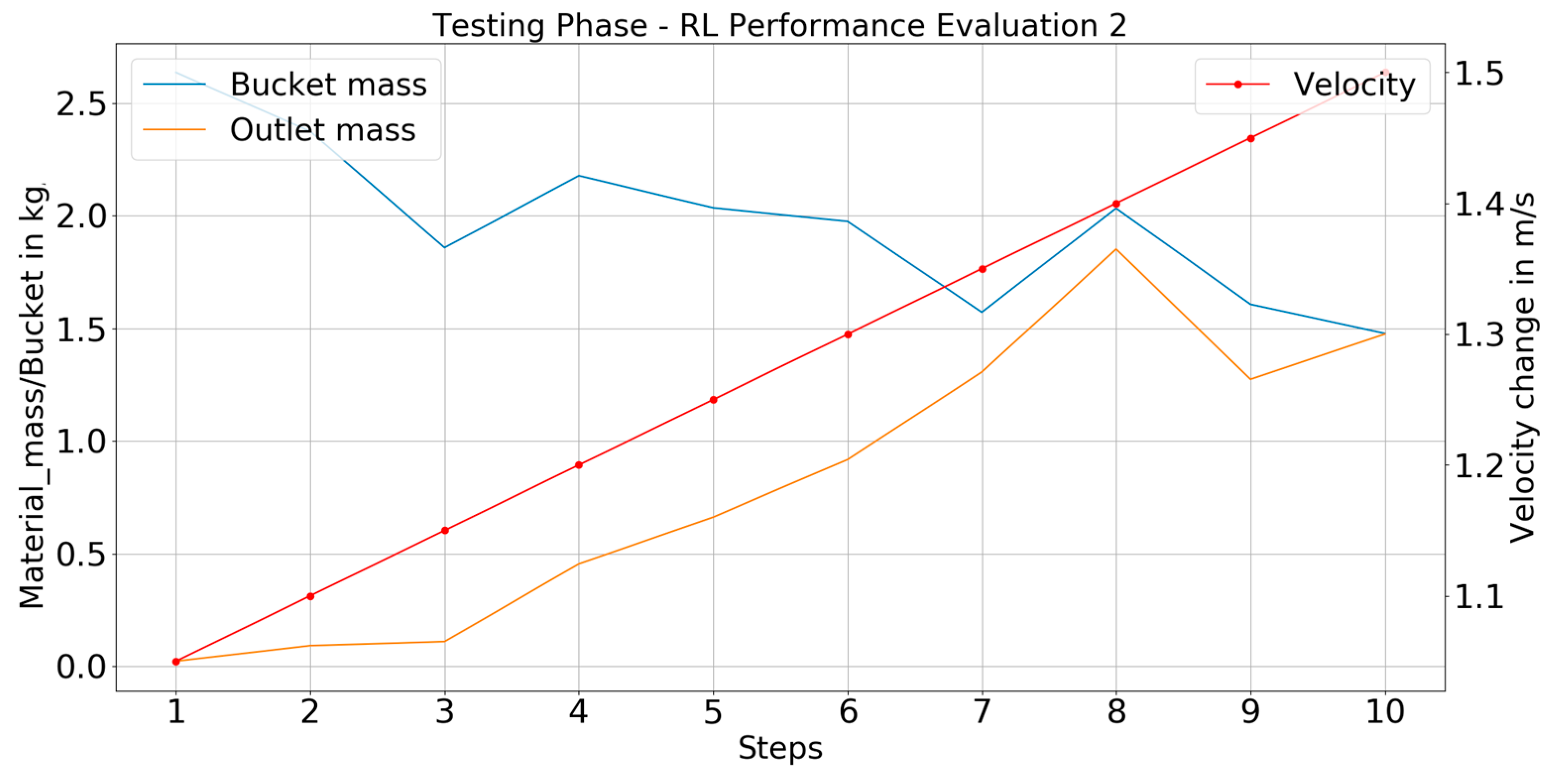
The RL-based optimization process was conducted by observing four important parameters that define the system state at a given instance. These parameters are the magnitude of the current velocity of the bucket elevator, the type of material in the system, the infeed rate of the material, and the PSD of the infeed material. Of these parameters, the infeed rate of the material was kept static and should be further manipulated in future tasks to make the optimization process more robust. Based on the values of these four parameters, the RL system formed a feedback control loop to monitor them and keep the discharge of the material at the outlet at an optimum level. The comparison between the mass of material within a filled bucket at the inlet and the discharge at the outlet was used as a measure to indicate if the system’s process was carried out in a planned manner. This material mass measurement did not have any impact on the RL algorithm itself.

This proposed approach was implemented using the A3C RL algorithm. This powerful algorithm allows the training to be conducted across multiple processors parallelly, wherein each processor was running its own unique DEM-based environment. Thus, a complete use of the available computation power was achieved.

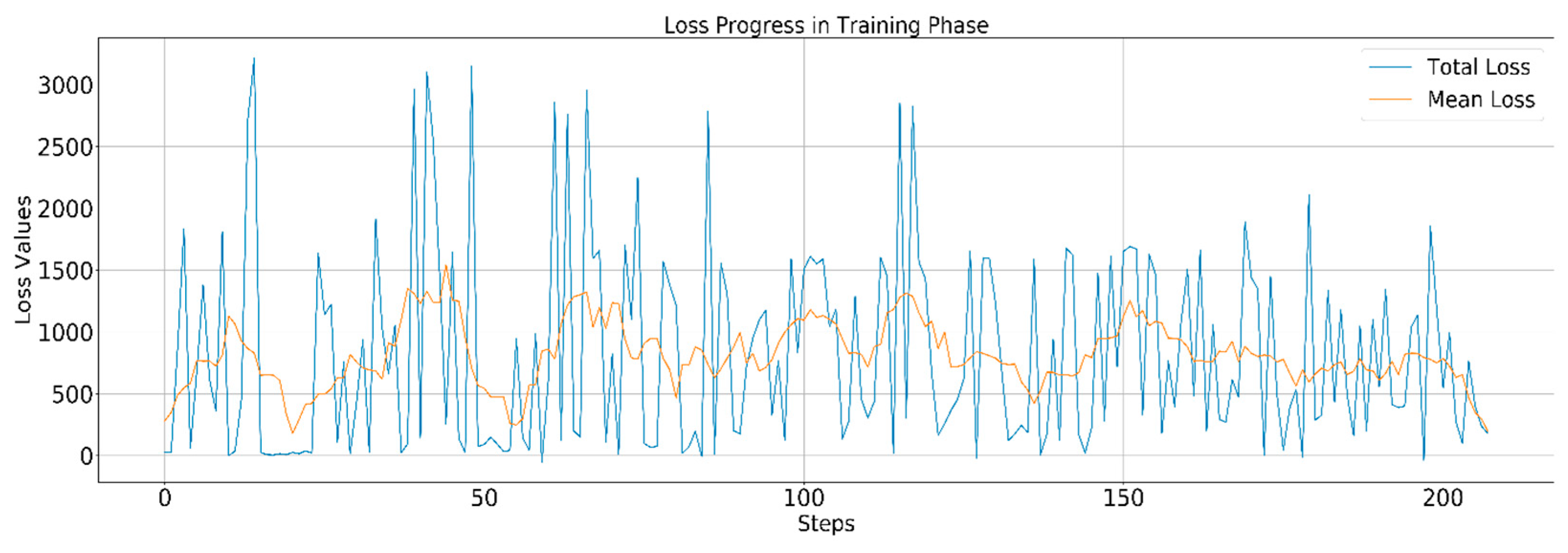
The results obtained in the training phase indicate that this approach to monitoring and optimizing the bucket elevator system using reinforcement learning is practical and usable. With a throughput that transferred 95% of the inlet material within a bucket at the outlet section, it proves the approach to be promising for making the bucket elevator system intelligent.

5. Future Scope

The optimization process of the bucket elevator system can be further boosted by considering the infeed material rate. Here, one can use a multi-objective optimization approach to monitor and control both the infeed rate and bucket velocity parameters. Certain provisions have already been made in the code to consider this in the future.

With the approach proposed by Mr. Elbel, it is possible to generate the DEM parameters replicating the behavior of AFR particles in the simulation. As such, this idea can be used to obtain the simulated behavior of different AFR particles and further optimize their usage in the bucket elevator system using the combination of DL and RL approaches discussed in this work.

One of the roadblocks to training with the RL approach for a satisfactory number of episodes was the allowance of the usage of only CPU cores in the Virtual Machine to run the DEM simulation. The possibility of running this DEM-based simulation on a Graphical User Interface (GPU) needs to be explored. With such a provision, it is possible to make full use of the GPU VRAM cores along with the CPU cores to increase the computational efficiency of the DEM simulation.

The DEM simulation is based on the Lagrangian method that involves solving trajectories or movements of each particle over time within the simulation. This means a higher degree of computation in the background. With a plan to develop a miniature prototype of a bucket elevator system, the use of such a prototype to train the RL agent can be explored. The training involved in such a setup will be a real-time inference and will drastically reduce the training time compared to the time needed in a DEM setup. If the prototype functions similarly to the actual bucket elevator system, the information learned by the RL agent using such a setup can be easily transferred and scaled to the actual system. Hereon, with only a few additional training episodes, the bucket elevator system will be functionally able to intelligently carry out its task. Thus, the training cost can be reduced to a great extent.

References

1. Aufderheide, D.; Di Matteo, L. Increasing Alternative Fuel Utilisation at Phoenix Cement. Cem. Int. 2020, 18, 2–8. [Google Scholar]
2. Paglia, C. Cement, Materials, Waste and Ashes: An Effort to Reduce CO2 Emissions. WEKA Industrie Medien, 14 July 2022. Available online: https://waste-management-world.com/resource-use/cement-materials-waste-and-ashes-an-effort-to-reduce-co2-emissions/ (accessed on 16 February 2023).
3. Vogelbacher, M.; Waibel, P.; Matthes, J.; Keller, H.B. Image-Based Characterization of Alternative Fuel Combustion with Multifuel Burners. IEEE Trans. Ind. Inform. 2018, 14, 588–597. [Google Scholar] [CrossRef]
4. Hassanpour, A.; Pasha, M. Discrete Element Method Applications in Process Engineering; CRC Press: Boca Raton, FL, USA, 2015. [Google Scholar]
5. Zegzulka, J. Bucket Elevator Filling and Discharge. In Discrete Element Method in the Design of Transport Systems; Springer: Berlin/Heidelberg, Germany, 2019. [Google Scholar]
6. Chikelu, P.O.; Nwigbo, S.C.; Obot, O.W.; Okolie, P.C.; Chukwuneke, J.L. Modeling and simulation of belt bucket elevator head shaft for safe life operation. Sci. Rep. 2023, 13, 1083. [Google Scholar] [CrossRef] [PubMed]
7. Ramrath, A. Kameragestützte Auswertung des Austragsverhaltens von Becherwerken; South Westphalia University of Applied Sciences: Soest, Germany, 2021. [Google Scholar]
8. Coetzee, C.J. Review: Calibration of the discrete element method. Powder Technol. 2017, 310, 104–142. [Google Scholar] [CrossRef]
9. Zhu, H.P.; Yhou, Z.Y.; Yang, R.; Yu, A. Discrete particle simulation of particulate systems: A review of major applications and findings. Chem. Eng. Sci. 2008, 62, 5728–5770. [Google Scholar] [CrossRef]
10. Chavan, A.; Aufderheide, D.; Schmidt, A.; Klopries, H. Synthetic Image Generation for Visual Particle Size Distribution Estimation based on U-NET Convolutional Networks. In Proceedings of the International Conference on Device Intelligence, Computing and Communication Technologies, (DICCT), Dehradun, India, 17–18 March 2023. [Google Scholar]
11. Ronneberger, O.; Fischer, P.; Brox, T. U-Net: Convolutional Networks for Biomedical Image Segmentation. In Medical Image Computing and Computer-Assisted Intervention (MICCAI); Springer: Berlin/Heidelberg, Germany, 2015; Volume 9351, pp. 234–241. [Google Scholar]
12. Ghali, R.; Akhloufi, M.A.; Jmal, M.; Mseddi, W. Wildfire Segmentation Using Deep Vision Transformers. Remote Sens. 2021, 13, 3527. [Google Scholar] [CrossRef]
13. Sutton, R.S.; Barto, A.G. Reinforcement Learning: An Introduction; MIT Press: Cambridge, MA, USA, 2018. [Google Scholar]
14. Kloss, C.; Goniva, C.; Hager, A.; Amberger, S.; Pirker, S. Models, algorithms and validation for opensource DEM and CFD- DEM. Prog. Comput. Fluid Dyn. 2012, 12, 140–152. [Google Scholar] [CrossRef]
15. Gelnar, D.; Zegzulka, J. Discrete Element Method in the Design of Transport Systems; Springer: Ostrava, Czech Republic, 2019. [Google Scholar]
16. Minaee, S.; Boykov, Y.; Porikli, F.; Plaza, A.; Kehtarnavaz, N.; Terzopoulos, D. Image Segmentation Using Deep Learning: A Survey. IEEE Trans. Pattern Anal. Mach. Intell. 2022, 44, 3523–3542. [Google Scholar] [CrossRef] [PubMed]
17. Vaswani, A.; Shazeer, N.M.; Parmar, N.; Uszkoreit, J.; Jones, L.; Gomez, A.N.; Kaiser, L.; Polosukhin, I. Attention is All you Need. Advances in neural information processing systems. 2017, 30. [Google Scholar]
18. Valeti, D. DBSCAN Algorithm for Fraud Detection & Outlier Detection in a Data Set. Medium, 18 October 2021. Available online: https://medium.com/@dilip.voleti/dbscan-algorithm-for-fraud-detection-outlier-detection-in-a-data-set-60a10ad06ea8 (accessed on 20 April 2023).
19. Mnih, V.; Badia, A.P.; Mirza, M.; Graves, A.; Lillicrap, T.; Harley, T.; Silver, D.; Kavukcuoglu, K. Asynchronous Methods for Deep Reinforcement Learning. In Proceedings of the 33rd International Conference on Machine Learning, New York, NY, USA, 19–24 June 2016. [Google Scholar]
20. Huynh, N. Understanding Evaluation Metrics in Medical Image Segmentation. Medium, 1 March 2023. Available online: https://medium.com/mlearning-ai/understanding-evaluation-metrics-in-medical-image-segmentation-d289a373a3f (accessed on 12 July 2023).
Figure 1. Bucket elevator: (a) real, (b) simulation.
Sustainability 16 03452 g001
Figure 2. Typical AFR resources used as a heat source, e.g., in the cement industry: (a) plastic waste, (b) rubber pieces (e.g., from shredded tires), (c) carpet and cloth waste, (d) biomass, (e) wood chips.
Sustainability 16 03452 g002
Figure 3. Process framework.
Sustainability 16 03452 g003
Figure 4. Simulated bucket elevator—Red outline shows the observed outlet of the elevator.
Sustainability 16 03452 g004
Figure 5. Sample background manipulated particle image: (a) original particle; (b) manipulated particle image; (c) manipulated particle mask.
Sustainability 16 03452 g005
Figure 6. Synthetic dataset sample: (a) image; (b) ground truth.
Sustainability 16 03452 g006
Figure 7. UNET architecture.
Sustainability 16 03452 g007
Figure 8. TransUNET architecture.
Sustainability 16 03452 g008
Figure 9. Variants of LIGGGHTS simulation (RL environment): (a) wood; (b) paper.
Sustainability 16 03452 g009
Figure 10. State space.
Sustainability 16 03452 g010
Figure 11. Reward calculation window—The red outline marks the undesired material area.
Sustainability 16 03452 g011
Figure 12. Working principle of A3C.
Sustainability 16 03452 g012
Figure 13. RL agent architecture.
Sustainability 16 03452 g013
Figure 14. UNET training and evaluation plot.
Sustainability 16 03452 g014
Figure 15. UNET dice score plot.
Sustainability 16 03452 g015
Figure 16. TransUNET training and evaluation plot.
Sustainability 16 03452 g016
Figure 17. TransUNET dice score plot.
Sustainability 16 03452 g017
Figure 18. Synthetic Samples: (a) image; (b) ground truth; (c) UNET prediction; (d) TransUNET prediction.
Sustainability 16 03452 g018
Figure 19. Real samples: (a) image; (b) UNET prediction; (c) TransUNET prediction.
Sustainability 16 03452 g019
Figure 20. Training phase—earned reward.
Sustainability 16 03452 g020
Figure 21. Training phase—overall loss.
Sustainability 16 03452 g021
Figure 22. Training phase—policy and value loss.
Sustainability 16 03452 g022
Figure 23. Testing phase—wood simulation.
Sustainability 16 03452 g023
Figure 24. Evaluation of optimization process (simulation type: wood)—Green area marks the desired material outlet region and red area indicates undesired region for material appearance.
Sustainability 16 03452 g024
Figure 25. Testing phase—paper simulation.
Sustainability 16 03452 g025
Figure 26. Evaluation of optimization process (simulation type: paper)—Green area marks the desired material outlet region and red area indicates undesired region for material appearance.
Sustainability 16 03452 g026