Vineyard Microclimatic Zoning as a Tool to Promote Sustainable Viticulture under Climate Change

Abstract

Understanding microclimate spatial variability is crucial for sustainable and optimised grape production within vineyard plots. By employing a combination of a microclimate model (NicheMapR) and multiple climate data sources, this study aimed to achieve microclimatic analysis in two vineyard plots, Quinta do Bomfim (northern Portugal) and Herdade do Esporão (southern Portugal). This approach provides an innovative 10 m spatial resolution for climate variables. This study incorporated local station hourly data with quantile mapping bias correction on the ERA5-land data. The microclimate model output was employed to perform bias correction on a EURO-CORDEX model ensemble. Climate extreme and bioclimatic indices specifically targeted to viticulture were calculated for each vineyard plot. The 10 m scale was analysed to identify potential shifts in temperature extremes, precipitation patterns, and other crucial climatic variables for grape cultivation within each specific plot. The significance of microclimate analyses was higher in areas with intricate topography, while in areas with smooth slopes, the variation of climatic variables was determined to be negligible. There was a projected increase in the median temperature of approximately 3.5 °C and 3.6 °C and a decrease in precipitation of approximately 98 mm and 105 mm in Quinta do Bomfim and Herdade do Esporão, respectively, when comparing a future scenario for the period 2071–2100 against the historical period (1981–2010). Hence, this study offers a comprehensive and future-oriented method for analysing microclimates in vineyard plots. By incorporating geospatial data, ERA5-land data, and the microclimate NicheMapR model, this research aimed to enhance the understanding of current microclimates and future climate scenarios for viticulturists.

1. Introduction

Over the past several decades, climate change has been attributed to anthropogenic forces acting on the climate system, with the increasing atmospheric concentrations of greenhouse gases and land use development caused by deforestation, desertification, and urbanisation being the two major drivers [1,2].

Climate change has a significant impact on all crops, and its effects are particularly pronounced for crops like grapevines [2]. Warmer temperatures are the most obvious consequence of this situation [3]. As a result of this shift, the entire cycle of wine grape growth is occurring earlier than usual. This includes the stages of budding, flowering, fruit-set, veraison, and harvest, all of which are currently occurring approximately ten days to two weeks earlier than their typical timing [4]. The ongoing increase in temperature implies that the alcohol levels tend to be higher, the acidity levels lower, and the tannins, which often ripen later, are found to be less refined [5]. Once the air temperatures surpass 35 °C, vines experience heat stress, which consequently leads to a decline in the production of secondary metabolites, a decrease in photosynthetic rates, and a reduction in vegetative growth [6]. This presents a problem for winegrowers who struggle to reach a balance between production and wine quality [7]. Furthermore, winters are also becoming significantly milder, causing grapevines to come out of dormancy earlier and making them more vulnerable to frost [8,9].

In xeric areas, where winters are moist and cool and summers are dry and warm, such as the Mediterranean region, vineyard soils are often the focus of attention to reduce competition between grapevines and the surrounding flora for essential resources such as water and nutrients [10,11]. Commonly used agricultural practices, such as herbicides’ application and intensive tillage [12], have the potential to affect soil quality and erosion and the overall sustainability of wine production [13], by affecting heat transfer and water storage, thus playing an important role in wine typicity [14].

While climate and soil are commonly considered the primary drivers of terroir on a regional level, many studies have emphasised the influence of topographical features such as elevation, slope, and aspect in the specific characteristics of wine at a local scale [15,16,17,18]. These topographical features have a significant impact on temperature profiles within a specific vineyard and are essential in the transition from macroclimate (i.e., larger region) to mesoclimate (i.e., specific vineyards) and to microclimate (i.e., individual rows of vines within the vineyard). The study of meteorological variables at the microscale can be a relevant tool for winegrowers to make well-informed decisions in the definition of their management strategies [19,20,21], and it becomes fundamental when it comes to adapting to the effects of climate change [2,22,23]. Innovative approaches are crucial for managing vineyards due to the complex relationship between microclimates and viticulture, especially in the face of climate change. Advanced microclimate models [24], sensor technology [25], and drone-based monitoring systems [26] can transform how viticulturists comprehend and adjust to changing environmental conditions in vineyards. Using microclimatic zoning allows the identification of environmental variations in vineyards, yielding valuable information on the climatic factors that impact the growth of grapevines [27,28]. However, we also recognise the potential of sensor technologies and drones to augment our understanding of microclimatic variations [29,30,31,32,33]. Despite the higher costs associated with sensors, their ability to collect real-time data provides invaluable insights into local environmental conditions. Similarly, the use of drones with specialised sensors allows for aerial monitoring, providing a complete understanding of vineyard microclimate. Nonetheless, these tools are not always available and can only be used in real-time monitoring of microclimates (not in forecasting or climate change projections).

The present study applied a microclimate model, NicheMapR [34], which combines physical elements, meteorological station data, and reanalysis of climate data to reproduce hourly temperature and precipitation data at a 10 m spatial resolution, within illustrative vineyard plots of two different terroirs in Portugal. With these data, we assessed potential climate change impacts by using two distinct representative concentration pathway scenarios. Additionally, the calculation of climatic and bioclimatic indices was performed to evaluate the spatial and temporal variability within each vineyard plot. This serves as a support system tool for decision-making, specifically concerning climate change and its effects on vineyards. Its purpose is to enhance the understanding of climate change among viticulturists, policymakers, and other relevant stakeholders, ultimately assisting them in their adaptation planning and eventually promoting sustainable viticultural practices.

2. Materials and Methods

2.1. Study Area Characterisation

Two vineyard plots located in two different terroirs in Portugal were the target of this study (Figure 1). The first plot features a vertical distance of around 70 m and is part of “Quinta do Bomfim” (QB, herein) which is located in the Douro region (Figure 1b,d), a region known for its intricate topography. This plot covers an area of 0.02 km² and is characterised by variations in direct sunlight due to mountains casting shadows throughout the day. The other plot belongs to “Herdade do Esporão” (HE, herein), located in the Alentejo region, southern Portugal (Figure 1c,e), and exhibits a predominantly flat terrain with a vertical distance of approximately 7 m. Consequently, the daily climatic conditions throughout the entire plot, covering an area of approximately 0.05 km², remain nearly unchanged. In the QB and HE plots, the grown grapevine cultivar is “Touriga Franca” and “Touriga Nacional”, respectively.

In terms of irrigation for the QB plot, it is important to note that currently no irrigation is being utilised, despite the presence of an installed irrigation system. The conduction system utilised in this particular setup is Royat, which involves a unilateral cordon and a density of 2900 plants per hectare, with a loam soil texture. In order to meet the plants’ needs, the HE plot utilises irrigation. The conduction system employed is a bilateral cordon with a density of 2222 plants per hectare. There is a distance of 3 m between lines and 1.5 m between plants. The plot is characterised by a sandy loam soil texture.

2.2. Microclimate Model

Microscale climate conditions depend on relevant processes, such as heat and mass exchange, air temperature, wind speed, humidity, short- and long-wavelength radiation, as well as soil moisture [35]. Noteworthy habitat features, including canopy shade, terrain, hill shade, and vegetation, are essential in effectively replicating microclimate conditions with precision. For microclimate modelling and calculating hourly air temperature in the vineyard plots, the NicheMapR package of the R programming environment was used [34]. One of the key features of the NicheMapR package is the inclusion of different model categories, such as plant models, endotherm models [36], ectotherm models [37], and dynamic energy budget models [38]. Its primary application is to provide hour-by-hour predictions of various climate variables, including air temperature, relative humidity, wind speed, soil moisture, and temperature. Solar radiation is among the routines used in this calculation and considers shading effects as hill shade, aspect, and slope. The NicheMapR package relies on the presence of various libraries, which are required for it to run properly. Data collection for microclimate modelling with high-resolution climate-forcing data implied the use of MCERA5 [39], a library from the R programming language. The combination of MCERA5 with the NicheMapR package, using ERA5-Land data, allows the computation of predictions for a local microclimate [40]. In addition to the installation of MCERA5, we also installed the complementary package ECMWFR [41]. This package allows access to climate datasets from Copernicus’s Climate Data Store, which can be found at https://cds.climate.copernicus.eu (accessed on 12 June 2023) [40]. The package LUBRIDATE [42] was used to work with and properly format dates and times from the climate datasets. Additionally, the use of DPLYR [43] significantly enhanced computation time in data manipulation, while TIDYNC [44] was a useful tool for manipulating binary data, specifically NetCDF files [45]. The function ‘get_dem’ from the microclima R package, which uses the R package ELEVATR [46], produces a digital elevation model (DEM) for a defined area. In this study, the DEM was retrieved for both vineyard plots. This enabled the incorporation of local orographic features, such as latitude, slope, and aspect, which combined with climatic factors, such as surface radiation, wind components, dew-point temperature, and cloud cover (Figure 2a), allowing the downscaling of ERA5-Land hourly 2 m air temperature data from a 10 km spatial resolution to a spatial resolution of approximately 10 m.

One of the key features of the R package NicheMapR is its incorporation of a generalised version of one of the earliest mechanistic models [47]. Extensive testing has been conducted in a wide array of settings to validate its relevance and efficiency [48,49,50,51,52,53,54,55,56], which ultimately led to its inclusion in this study. All parameters were set by coupling the vineyard plots’ spatial coordinates with a 10 m spatial resolution DEM, which was then used to calculate the topographical features for the downscaling of the climate data.

2.3. Climate Data

For this study, three periods were carefully selected: 1981–2010, which serves as a historical reference, and two future periods, namely 2041–2070 and 2071–2100 under two different scenarios, the Representative Concentration Pathways (RCP), namely RCP4.5 and RCP8.5 [57], thus representing a moderate and a severe climate scenario, respectively.

With the NicheMapR package, historical climate data from ERA5-Land (European Climate Rea-Analysis version 5) was retrieved for each vineyard plot from the Copernicus Climate Change Service, which provides a spatial resolution of approximately 10 km [58]. For each vineyard plot, we also collected the observed hourly precipitation and temperature station data from each partner (QB and HE) from 2000 to 2019. These data were used to bias correct the ERA5-Land data. This was conducted by applying quantile mapping, resorting to an R package named ‘qmap’ (Section 2.4). The future climate data used in this study were obtained from a series of experiments conducted by the EURO-CORDEX project. To mitigate uncertainty arising from different models, we employed an ensemble approach by using three distinct Regional Climate Models (RCMs), forced by three separate General Circulation Models (GCMs). Daily mean (TG), minimum (TN), and maximum (TX) air temperatures (in °C) and precipitation (RR) (in mm) time series were retrieved from the three chain experiment model datasets for both plots over the historical and future periods. The following chain experiments were considered: SMHIRCA4 driven by MPI-M-MPI-ESM-LR, DMI-HIRHAM5 driven by ICHEC-EC-EARTH, and CLMcom-CCLM4-8-17 driven by CNRM-CERFACS-CNRM-CM5 (under both RCP4.5 and RCP8.5) (Table S1). The same quantile mapping technique was applied between the output of the microclimate model and the series of experiments conducted by the EURO-CORDEX models to obtain bias-corrected data series of daily precipitation and temperature for the future periods (2041–2070 and 2071–2100) under both RCPs (Figure 2b).

2.4. Quantile Mapping

To perform the bias correction of the climate data (ERA5-Land vs. observed station data and EURO-CORDEX models vs. microclimate data output) the qmap R package was used [59]. It performs statistical transformations for processing climate model outputs using quantile mapping. The primary functions are ‘fitQmap’ and ‘doQmap’. The first identifies the parameters of different quantile mapping methods, while the second performs quantile mapping using the parameters identified previously. Four different quantile mapping methods were tested: (1) using parametric transformations (fitQmapPTF), (2) using smoothing spline (fitQmapSSPLIN), (3) non-parametric using robust empirical quantiles (fitQmapRQUANT) and (4) non-parametric using empirical quantiles (fitQmapQUANT).

The ‘fitQmapPTF’ function fits parametric transformations into the quantile-quantile relation. Subsequently, the ‘doQmapPTF’ function applies this transformation to adjust the distribution of the modelled data to match that of the observations. The ‘fitQmapSSPLIN’ function is used to fit a smoothing spline to the quantile-quantile plot of the observed and modelled time series. On the other hand, the ‘doQmapSSPLIN’ function applies the spline function to adjust the distribution of the modelled data so that it aligns with the distribution of the observations. To estimate the quantile-quantile relation values between observed and modelled time series for regularly spaced quantiles, the ‘fitQmapRQUANT’ function employs a local linear least square regression. Conversely, the ‘doQmapRQUANT’ function performs quantile mapping by interpolating the empirical quantiles. The ‘fitQmapQUANT’ function estimates the values of the empirical cumulative distribution function for both the observed and modelled time series. These estimates are calculated for regularly spaced quantiles. The ‘doQmapQUANT’ function uses these estimates to perform quantile mapping. Lastly, we chose the smoothing spline method based on the obtained performance metrics (Figure S1).

2.5. Agroclimatic Zoning

Climate data operators (CDOs) [60] allow the analysis and manipulation of climate data to calculate climatic indices, which are crucial tools for analysing and understanding climate patterns. Climatic indices play a major role in characterising different aspects of climate spatial and temporal variability. They provide quantitative measures that help in assessing the frequency, intensity, and duration of specific climate events. Understanding these indices is essential for climate policymakers and researchers to identify climate change impacts and develop effective mitigation and adaptation strategies. This approach enables a comprehensive analysis of temperature and precipitation, and their effects on vineyards, contributing to a better perception of climate variability and its implications for the wine sector. In this study, several climatic and bioclimatic indices were calculated: (1) the dryness index, (2) the hydrothermal index of Branas, Bernon and Levandoux, and (3) the Huglin Heliothermal index, as bioclimatic indices (Table S2), and (4) growing season length, (5) extreme summer days, and (6) tropical nights, as relevant climate extreme indices. Other temperature and precipitation indices are shown in Figures S2–S4 and their definitions are described in Table S3, in the Supplementary Material.

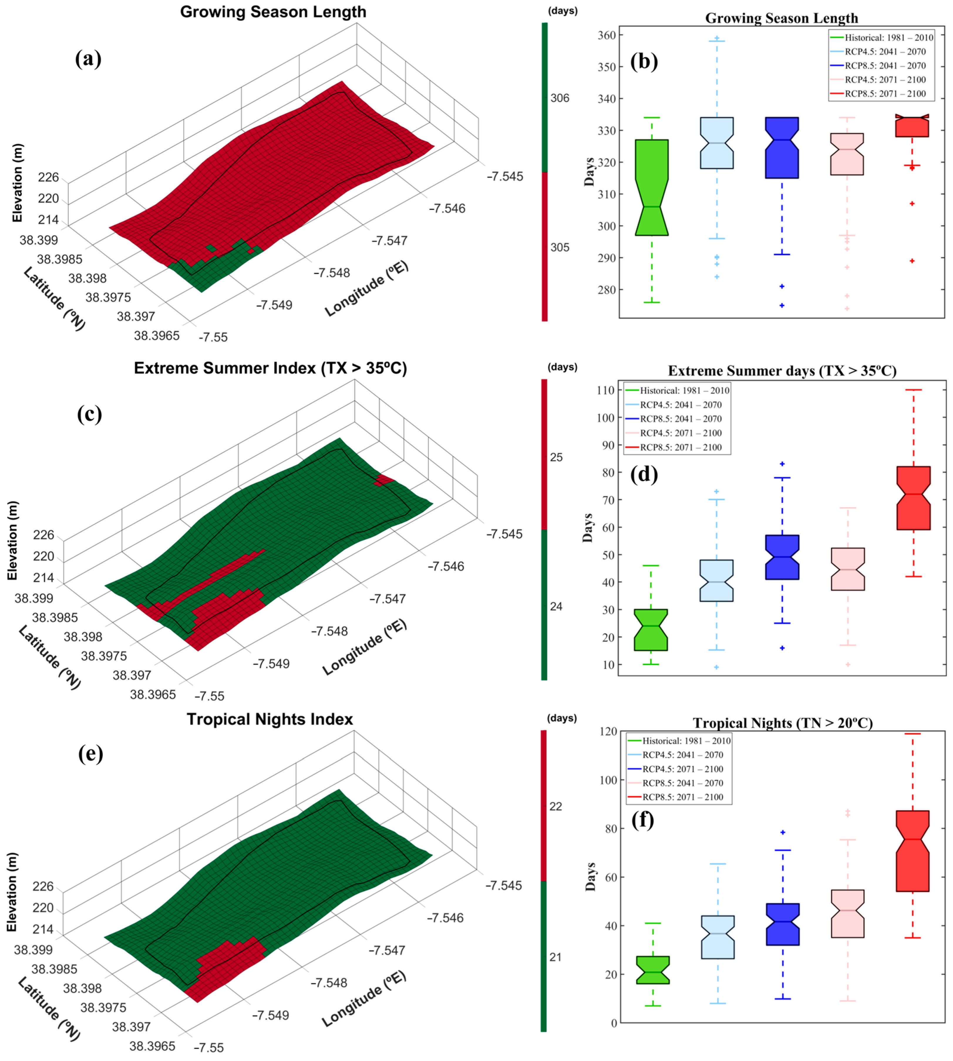
2.5.1. Growing Season Length

The Growing Season Length (GSL) is a climatic index that plays a major role in understanding favourable conditions for plant growth and development. In this study, it was defined as the period where, for 6 consecutive days, the minimum temperature was above 10 °C, which, for vineyards, is within the favourable range of plant growth [22]. GSL is also an essential indicator of agroforestry, providing insights into the duration of days for crops to complete their life cycles, and helping farmers determine suitable planting and harvesting times. It provides insight into the choice of grape cultivars or different crops that can be grown in a specific region and contributes to optimising agricultural practices for higher yields.

2.5.2. Extreme Summer Days

The summer days index measures the number of days with maximum temperatures exceeding a predefined threshold, typically 25 °C. In this study, we calculated extreme summer days (temperature above 35 °C) since it has a greater impact on vineyards [61], identifying trends in temperature changes during summer, and providing insights into heatwave occurrences.

2.5.3. Tropical Nights

The tropical night index quantifies the number of nights with minimum temperatures above a specified threshold, commonly 20 °C. It offers insights into night time temperature variations, crucial for assessing heat stress on plants.

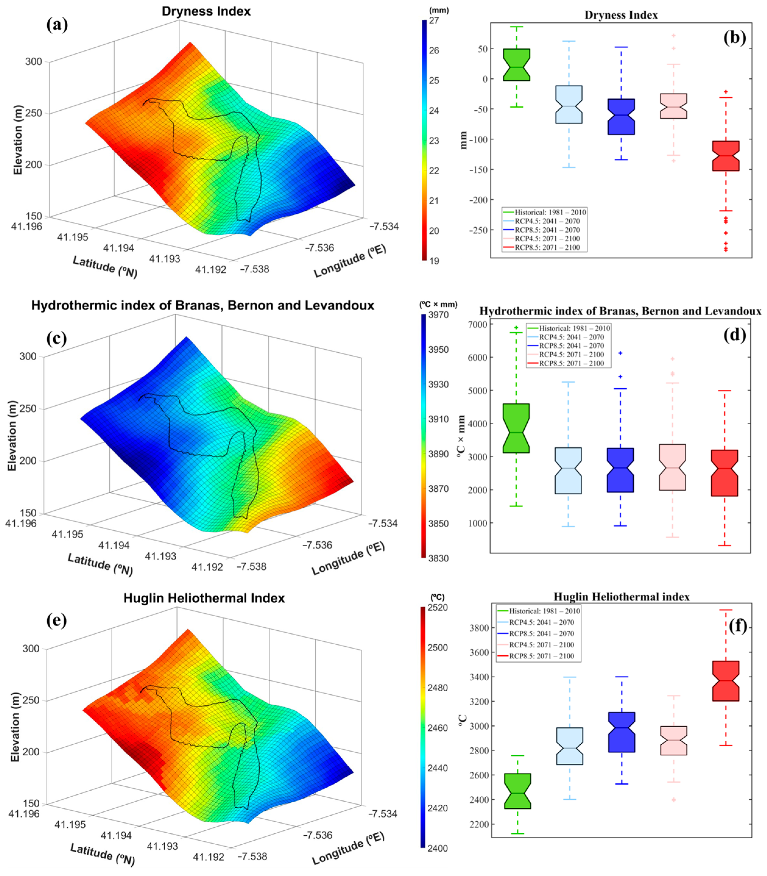
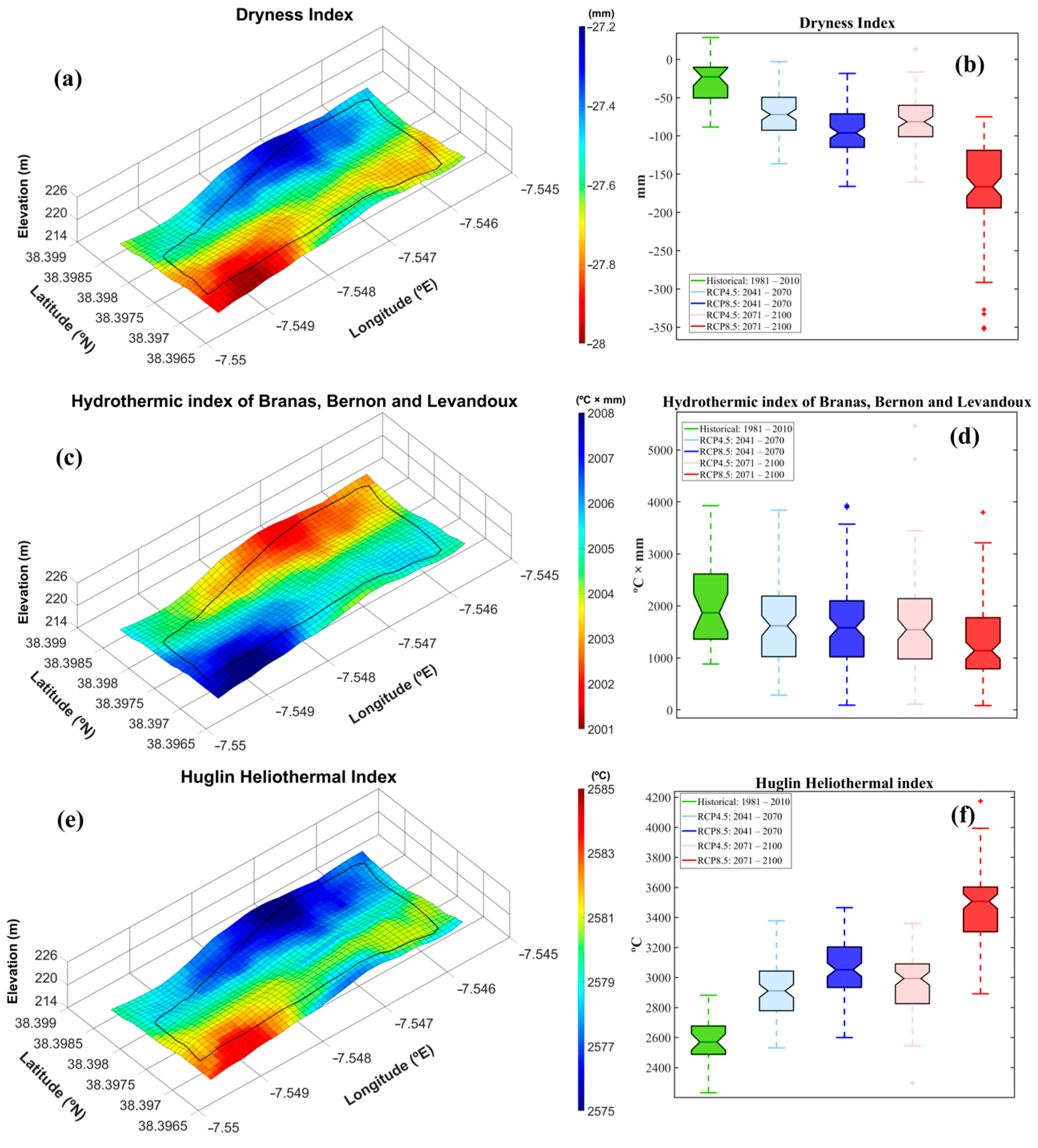
2.5.4. Huglin Heliothermic Index

The Huglin Heliothermic Index (HI) [62] is a bioclimatic heat index specifically designed for viticulture regions. It considers the heliothermic potential and calculates the temperature sum above 10 °C during specific periods, depending on the hemisphere. For the Northern hemisphere, the index considers the temperature sum from April until September, while for the Southern hemisphere, it considers the period from October until March. This index is particularly relevant when related to the phenological timings of grapevines, especially the maturation stage.

2.5.5. Hydrothermal Index of Branas, Bernon and Levandoux

The Hydrothermal Index of Branas, Bernon, and Levandoux (HIBBL) [63] considers the combined impact of temperature and precipitation on grape yield and the overall quality of the resulting wine. The index value is calculated by summing the products of the monthly mean temperature (°C) and the monthly accumulated precipitation amount (mm), over the period from April to September in the Northern Hemisphere or from October to February in the Southern Hemisphere. This index is known to be related to the potential risk of grapevine fungal diseases, such as downy mildew.

2.5.6. Dryness Index

The Dryness Index (DI) [64] was determined by using a modified version of Riou’s potential water balance of the soil index [65], specifically for vineyards. This method allows for the characterisation of the water component of the climate in a grape-growing region by considering factors such as evaporation and precipitation without deduction for surface runoff or drainage. This index provides a lower and upper threshold in defining the water requirements for grapevines.

3. Results

3.1. Microclimatic Characteristics

The ombrothermic diagram and the annual mean temperature and precipitation for the historical period for both vineyard plots at a 10 m spatial resolution are shown in Figure 3. As expected, the QB plot shows a more moderate climate in the summer than the HE plot, which is much dryer (Figure 3a,b). Although the temperature profile is very similar, QB shows more precipitation throughout the year when compared to HE. Further, the spatial variation in annual mean temperature modelled in QB (0.6 °C, Figure 3c) is greater than the one observed in HE (less than 0.1 °C, Figure 3d). On the other hand, precipitation variation in such small plots is negligible, with fluctuations between 1 and 2 mm (Figure 3e,f). Noteworthy, higher precipitation values co-occur with higher temperatures, highlighting the relevance of topographic features in determining the spatial correlation between these two critical variables.

Figure 4 shows the boxplots of the mean annual temperature and mean annual precipitation for both QB and HE for both future periods (2041–2070 and 2071–2100) and scenarios (RCP4.5 and RCP8.5). Maximum and minimum annual temperatures are shown in Figure S5. As expected, in line with the ongoing trend of climate change, we have observed an increase in temperature and a simultaneous decrease in precipitation in both vineyard parcels. There is a projected increase in the median temperature of approximately 3.5 °C and 3.6 °C and a decrease in precipitation of approximately 98 mm and 105 mm in QB and HE, respectively, when comparing the RCP8.5 scenario for the period 2071–2100 against the historical period. Topographic information (i.e., slope and aspect, can be found in Figure S6 in the Supplementary Material).

An ANOVA test to assess the overall variance among the datasets developed in this paper was conducted (Table S4). Subsequently, to identify specific differences between individual groups, we employed a post hoc Tukey–Kramer test (Table S5). Based on the results of the ANOVA (F-test = 5731) and Tukey–Kramer tests conducted, we found that all p-values were below 0.01, showing highly significant differences among the groups. Furthermore, examination of the means revealed each group exhibited statistically significant variations from one another. It can be inferred that the differences observed in the datasets developed in our study reflect meaningful distinctions in their characteristics.

3.2. Climatic Indices

The spatial variation shown in Figure 5 and Figure 6 is relative to the mean values of the entire historical period, while the boxplots show the yearly variation for all scenarios and future periods. The GSL index in QB (Figure 5a) varies between 284 and 302 days, mainly due to the topographic features observed in the Douro region (deep valleys and mountain shades). This leads to a strong temperature variation within the vineyard plot, where the northernmost part of the plot is subject to more hours per day of solar radiation than the southernmost part, which receives mountain shade. The median projected variation of the GSL (Figure 5b) is expected to increase between 320 days (RCP4.5; 2041–2070) and 330 days (RC8.5; 2071–2100), due to the increasing temperature projected by the climate change models. The increase in temperature also brings other challenges, such as extreme temperature events, which were analysed by calculating the extreme temperature index and the tropical night index. The extreme temperature index (Figure 5c) followed a similar spatial pattern to the GSL, with the northwestern area of the plot having summer days more often with TX higher than 35 °C than the southeastern area. For the historical period, this index varied between 18 and 21 days, with median values ranging between 38 days under RCP4.5 and 65 days under RCP8.5, and a maximum value of 115 days for RCP8.5 considering the 2071–2100 period. At night, the spatial variation of TN (tropical night index, Figure 5e) was similar to the one observed for the extreme temperature index, meaning that during the night, the warmer areas occurred more often in the north and northwesternmost part of the vineyard plot (Figure 4e), with values varying between 15 and 21 days for the historical period and an expected increase to 38 and 62 days for future scenarios (RCP4.5 and RCP8.5, respectively). Figures S2 and S3 in the Supplementary Material show other climatic indices, with their spatial and temporal distribution, for the QB plot.

Concerning the spatial variation of these indices for the HE, albeit minimal (Figure 6a,c,e), higher values are observed in the southwestern most part of the plot with values for the historical period varying between 305 and 306 days, 24 and 25 days, and 21 and 22 days for the GSL, extreme summer index, and tropical nights, respectively. This can be explained by the homogeneous topography observed in HE. Also, since HE is usually warmer than QB, these values are higher than QB for both historical and future scenarios. In the HE plot, the GSL is expected to increase to 326 and 332 days (Figure 6b), the extreme summer index to 40 and 71 days (Figure 6d), and the number of tropical nights to 38 and 73 days (Figure 6f) under RCP4.5 (2041–2070) and RCP8.5 (2071–2100), respectively. Figure S3 in the Supplementary Material shows other climatic indices and their temporal distribution for the HE plot not mentioned here (it is worth mentioning that the HE plot has no significant spatial variation).

As mentioned previously, the spatial variation of precipitation at such a high resolution and for such small areas does not reveal major changes; therefore, the spatial variation of the precipitation indices is almost null, particularly in HE. Still, the temporal variation for both plots is presented (Figures S3 and S4) and the median values are shown in

Table 1. Historical precipitation indices and expected precipitation indices under different future (2071–2100) climate scenarios (RCP4.5 and RCP8.5) in the QB and HE vineyard plots (bold values show statistical significance).

Index	QB			HE
	Historical	RCP4.5	RCP8.5	Historical	RCP4.5	RCP8.5
Precipitation (April–September) (mm)	255	169	160	150	103	81
Simple daily intensity index (mm)	7	7	8	6	6	7
Precipitation days above 20 mm (days)	7	7	7	3	3	4
Precipitation days above 30 mm (days)	1	2	2	0	1	1
Highest one-day precipitation (mm)	40	39	39	30	35	35

.

In both vineyard plots, QB and HE, precipitation in the favourable period (April to September) is expected to decrease, while temperature is expected to increase under both RCPs. The frequency of extreme precipitation events is likely to increase, as shown by the increment in the number of days with precipitation above 30 mm for both plots and climate scenarios. As for the severity of extreme precipitation events, the maximum precipitation occurring in one day is expected to slightly increase in HE, while remaining virtually unchanged in QB. All boxplots provide a visual representation that effectively shows the level of uncertainty surrounding the median (notch) for all of the indices. The fact that the notches of all of the precipitation indices (except precipitation April–September, between the historical and future periods,Figures S3c and S4e) overlap shows that there is not enough evidence to support a significant difference in the medians.

3.3. Bioclimatic Indices

In the current conditions, both plots fall within the moderately dry category according to the DI (Table S2), although the HE plot exhibits slightly higher levels of dryness (Figure 7 and Figure 8). While the variability of DI in the HE plot is negligible, there is a slight variation in the QB plot where the drier areas have a similar disposition to the highest values of the previously presented climatic indexes. Looking ahead, under future scenarios, both plots are projected to experience heightened dryness, which is particularly clear in the RCP8.5 scenario where the DI escalates from the moderately dry to the excessively dry class. This emphasises the need for irrigation to maintain grapevine suitability.

Regarding the risk of fungal diseases, such as downy mildew, under historic conditions, the HIBBL shows a moderate risk in the QB plot, where there is some spatial variation, and a low risk in the HE plot, where HIBBL is practically constant. Of note, the higher risk areas for fungal diseases in the QB plot occur in the northwestern part of the plot, coinciding with higher drier index values, although with increased precipitation, thus higher values of HIBBL. Under future climate conditions, the HIBBL values are expected to decrease, showing a reduced risk of such diseases. These shifts are attributed to the expected decreases in precipitation and humidity under future climate scenarios.

The results show that for both plots, the HI currently falls within the warm category. The spatial variability of HI occurring in the QB and HE plots is enough to present some management challenges, especially in the planning of phenology-dependent activities. However, with projected future climate change, both plots should transition towards the “too hot” classification, potentially posing additional threats and challenges.

Despite the enhanced resolution, the spatial variability of bioclimatic indices within each plot is not enough for class differentiation. Consequently, the plots are grouped into the same classes for HI, HIBBL, and DI, primarily due to the limited study area.

4. Discussion

4.1. Microclimate

NicheMapR was demonstrated to be a powerful tool for perceiving microclimate changes in small areas, such as vineyards. Its integration with historical weather data, geospatial data, global aerosol data, and site properties provides insights into understanding the vineyard environment. The results obtained using NicheMapR show that topography plays a major role in temperature variation, depicting the effect of radiation and mountain shade (not disregarding wind profiles). Thus, the microclimate model can depict differences in temperature in relatively small areas. It can help vineyard managers anticipate and adapt to these changes by identifying different microclimates for future planting or implementing adaptation measures for long-term sustainability [66,67]. Overall, NicheMapR can be a useful decision tool that provides insights for crop management, enhancing decision-making processes, and ultimately improving vineyard sustainability.

4.2. Extreme Climatic Indices

4.2.1. Growing Season Length

The GSL plays a crucial role in determining grape ripening and lifecycle. Shorter growing seasons may lead to incomplete grape ripening and increased acidity, affecting the flavour and thus affecting the quality of the wine [22]. Conversely, longer growing seasons may provide enough time for grapes to reach optimal ripeness, potentially enhancing wine quality, though over-ripeness can lead to elevated sugar levels and thus higher alcohol content [68]. An expansion of this season may lead to earlier germination or budbreak (and consequently other phenological stages). Earlier germination or sprouting can increase the likelihood of frost damage, even if the frequency of late frosts does not increase and there is no change in the period in which they occur. Conversely, at the end of the vegetative cycle, the temperatures may not drop enough to start the dormancy period. The year 2023 at HE was marked by an interesting observation, where the vines began a new vegetative cycle in the post-harvest period. However, this growth was cut short due to the absence of suitable conditions for further development. This index helps viticulturists to make informed decisions on adaptation strategies for a particular region, such as planting and harvesting dates or the selection of different cultivars [23]. GSL also gives insights into determining the chilling requirement for the dormancy period, affecting the timing of budburst [69]. In the future, GSL is expected to increase in both QB and HE, challenging the adequate grape maturation but decreased dormancy period.

4.2.2. Extreme Summer Days

Excessive heat can lead to increased sugar accumulation in grapes, potentially leading to higher alcohol levels [70], but it can also cause stress to the grapevines [71], resulting in maturation stoppages [72]. Vineyard management strategies, such as canopy management [73] and irrigation [74], may need to be adjusted to mitigate the effects of extreme heat to achieve the wine characteristics of the region. Shading nets and kaolin applications are two common practices that offer distinct benefits, ranging from protection from extreme weather to pest management [75]. Despite the projected increase of days with very high temperatures, cv. “Touriga Nacional” and cv. “Touriga Franca” are known for their ability to adapt to environmental stresses, particularly due to their capacity to withstand high light intensities. This characteristic enables them to better adjust to warm conditions, as long as sufficient water is provided [76], though they are still subject to yield losses. With temperatures expected to rise, pests are also expected to develop more quickly, producing more generations per year, increasing the intensity of their attacks and, consequently, increasing the damage to vineyards. The challenges in vineyard management are further compounded by the anticipation of pests “arriving” and the subsequent rise in the intensity of attacks.

4.2.3. Tropical Nights

Tropical nights (high minimum temperatures) influence grapevine respiration and metabolic processes, causing a decrease in the overall carbohydrate contents of the leaves [77] and an alteration in the balance between sugar accumulation and acid degradation [78], as well as aromatic profiles [79]. Future climate data shows that the minimum values of tropical nights coincide with the maximum values of the historical period. While in HE the spatial variation in the plot is minimal, in the northernmost area of the plot in QB, tropical nights are expected to become more prevalent due to climate change. Vineyard practices may need to be adapted to maintain the desired balance in grape composition when compared to the rest of the plot.

4.2.4. Precipitation Indices

In both plots, an overall decrease in precipitation is expected, although days with higher precipitation are expected to increase, which may lead to more erosion events [80]. Noteworthy, the median values of the boxplots for all periods and scenarios against historical periods show no statistical difference, except for the precipitation in the favourable periods (April to September) (Figures S3c and S4e), which are predicted to decrease considerably. The combined effect of drier and warmer conditions exacerbates plant stress even further, since evapotranspiration decreases, resulting in a higher temperature at the plant level (reduced latent heat) [81,82].

4.3. Bioclimatic Indices

Under future climate scenarios, these two vineyard plots are expected to undergo significant changes in climatic conditions, which may affect grape yields and quality attributes, ultimately affecting wine production. These variations include a projected increase in HI, a decreased HIBBL, and higher dryness. HI is likely to shift to the “too-warm class”, showing that the warmer temperatures may have profound effects on the grapevine phenological stages, potentially leading to earlier onset of bud break or accelerated ripening [83]. These aspects, combined with the impacts from the extreme temperatures (maturation stoppages, cf. Section 4.2.2), may have profound negative impacts on viticulture and winemaking. Furthermore, higher temperatures may bring changes to grape flavour profiles, influencing the typicity of wines produced by the plots [84,85]. The projected decrease in HIBBL, according to the index definition, shows lower risks of fungal pathogens and diseases, such as downy mildew. Both vineyard plots are projected to face increased dryness, driven by changes in precipitation patterns and rising temperatures. This heightened aridity, according to the index classification, may exacerbate water scarcity concerns, requiring irrigation and sustainable water management strategies to maintain typicity, yields and quality [86]. Hence, the future climatic conditions for plots QB and HE require proactive adaptation measures that will be essential for vineyard management in these plots to improve sustainability and produce high-quality wines amidst adverse climatic conditions.

4.4. Climate Change Scenarios

In the context of climate change scenarios like RCP4.5 and RCP8.5, these agroclimatic indices can serve as valuable tools for predicting future conditions. Although future scenarios suggest potential shifts in temperature and precipitation patterns, in smaller areas, such as the vineyard plots addressed here, the spatial climate change signal remains the same due to the spatial resolution of the future climate data. The increased temperature, reduced precipitation and a heightened occurrence of extreme weather events may lead to shifts in all of these indices, which can significantly affect viticulture in the future [87,88]. The occurrence of extreme heat events has the potential to cause sunburn on grape clusters, while extreme precipitation events represent an increasing risk of physical damage to grape clusters and of erosion potentially affecting the integrity of vertical vineyards due to landslides. An increase in temperature and decrease in precipitation may cause reduced soil moisture levels, altering the availability of nutrients and water stress in vineyards. This can intensify the flavours of the grapes, but it can also result in the formation of smaller berries and a reduction in the overall yield of grapes [89].

The agroclimatic indices mentioned here are highly valuable as they offer insights into a range of climatic parameters that have a direct impact on the growth of grapevines, the ripening of grapes, and ultimately, the overall quality of wine [90,91]. Adapting to these changes may involve implementing innovative viticultural practices, selecting suitable grape cultivars, and potentially exploring new terroirs [87]. Climate-smart viticulture, associated with a thorough understanding of agroclimatic indices, warrants the sustainability and resilience of vineyards in the face of climate change [7,78]. As a direct result of these changing climate conditions, it becomes important to continue to re-evaluate these agroclimatic indices and act accordingly to maintain the climate features that contribute to a specific terroir. If other strategies fail, these climatic scenarios may have the potential to restrict the growth of vineyards and require their relocation to higher altitudes [2].

4.5. Advantages and Disadvantages of Microclimate Models

Microclimate models offer advantages and disadvantages when compared to sensors or drones [25] for tracking small-scale temperature and precipitation fluctuations. By considering different environmental factors and inputs (heat and mass exchange, air temperature, wind speed, humidity, short- and long-wavelength radiation, soil moisture, canopy shade, terrain, hill shade, and vegetation), microclimate models can simulate and predict variations in temperature and precipitation. Once microclimate models are developed, they can offer a cost-effective alternative to continuously deploying sensors or drones [28,34,92]. These models can provide valuable insights over a larger geographical area, provided they undergo proper calibration and validation. Conversely, the development of microclimate models requires specialised knowledge in fields such as meteorology, climatology, and computational modelling, combined with the use of robust computational processing capabilities. For models to perform effectively, it is crucial to have accurate input data. However, this can be a challenge, particularly in remote or less-studied areas, where it may not always be available. When deciding between microclimate models, sensors, or drones, several factors come into play, including specific research or monitoring objectives, budget constraints, spatial scale, topography complexity, and data accuracy requirements. The most effective strategy for comprehensive environmental monitoring may often involve a combination of these approaches [93].

Despite the differences in approaches, both methods enable a thorough characterisation of microclimate conditions found within vineyard landscapes. This, in turn, aids in the identification of mesoclimatic variations, the exploration of potential climate change impacts, the evaluation of adaptation strategies, and the optimisation of vineyard management decisions, all of which contribute to enhancing the expression of terroir. These tools serve as invaluable tools for vineyard management, offering valuable insights into various aspects such as ideal planting locations, vineyard design, canopy management techniques, irrigation scheduling, and even determining the perfect time for harvest. Winegrowers obtain the ability to maximise grape quality and wine typicity by integrating terroir-specific information into their decision-making processes, which in turn contributes to the sustainability and resilience of the winegrowing industry.

5. Conclusions

The importance of microclimate modelling cannot be overstated, especially when it comes to determining agroclimatic indices for vineyards, particularly at a spatial resolution that aligns with the intricacies of vineyard landscapes, as shown in this study. In the HE vineyard plot, the spatial results are not very relevant because the terrain is mostly flat, with slight spatial gradients and the relevance of this modelling is not as valuable. However, in the QB vineyard plot, the significance merit of this type of modelling is clear, denoting important variations at such a small spatial resolution. The relationship between different climatic elements within a specific area may have a significant influence on the growth and development of grapevines, particularly in areas with complex topography, ultimately shaping the quality of the wine produced. To preserve the typicity of wines and terroirs, it is crucial to comprehend and adjust to the spatial variation of these agroclimatic indices when facing the ongoing climate. This can be achieved through a combination of sustainable viticultural practices and, in certain cases, a re-evaluation of grape cultivars and vineyard locations.

References

1. IPCC Climate Change 2022: Impacts, Adaptation and Vulnerability; Working Group II Contribution to the IPCC Sixth Assessment Report; IPCC: Geneva, Switzerland, 2022.
2. Jones, G.V.; Edwards, E.J.; Bonada, M.; Sadras, V.O.; Krstic, M.P.; Herderich, M.J. Climate Change and Its Consequences for Viticulture, Chapter 17. In Managing Wine Quality (Second Edition); Reynolds, A.G., Ed.; Woodhead Publishing: Cambridge, UK, 2022; pp. 727–778. ISBN 978-0-08-102067-8. [Google Scholar]
3. Kimani, B.K. Influence of Temperature Variations on Grapevine Phenology. Am. J. Agric. 2024, 6, 46–55. [Google Scholar]
4. Fraga, H.; Malheiro, A.C.; Moutinho-Pereira, J.; Santos, J.A. An Overview of Climate Change Impacts on European Viticulture. Food Energy Secur. 2012, 1, 94–110. [Google Scholar] [CrossRef]
5. Van Leeuwen, C.; Darriet, P. The Impact of Climate Change on Viticulture and Wine Quality. J. Wine Econ. 2016, 11, 150–167. [Google Scholar] [CrossRef]
6. Moutinho-Pereira, J.M.; Correia, C.M.; Gonçalves, B.M.; Bacelar, E.A.; Torres-Pereira, J.M. Leaf Gas Exchange and Water Relations of Grapevines Grown in Three Different Conditions. Photosynthetica 2004, 42, 81–86. [Google Scholar] [CrossRef]
7. Santos, J.A.; Fraga, H.; Malheiro, A.C.; Moutinho-Pereira, J.; Dinis, L.-T.; Correia, C.; Moriondo, M.; Leolini, L.; Dibari, C.; Costafreda-Aumedes, S. A Review of the Potential Climate Change Impacts and Adaptation Options for European Viticulture. Appl. Sci. 2020, 10, 3092. [Google Scholar] [CrossRef]
8. Poni, S.; Sabbatini, P.; Palliotti, A. Facing Spring Frost Damage in Grapevine: Recent Developments and the Role of Delayed Winter Pruning—A Review. Am. J. Enol. Vitic. 2022, 73, 211–226. [Google Scholar] [CrossRef]
9. Kovács, L.G.; Byers, P.L.; Kaps, M.L.; Saenz, J. Dormancy, Cold Hardiness, and Spring Frost Hazard in Vitis Amurensis Hybrids under Continental Climatic Conditions. Am. J. Enol. Vitic. 2003, 54, 8–14. [Google Scholar] [CrossRef]
10. Costa, J.M.; Egipto, R.; Aguiar, F.C.; Marques, P.; Nogales, A.; Madeira, M. The Role of Soil Temperature in Mediterranean Vineyards in a Climate Change Context. Front. Plant Sci. 2023, 14, 1145137. [Google Scholar] [CrossRef]
11. Giffard, B.; Winter, S.; Guidoni, S.; Nicolai, A.; Castaldini, M.; Cluzeau, D.; Coll, P.; Cortet, J.; Le Cadre, E.; D’errico, G. Vineyard Management and Its Impacts on Soil Biodiversity, Functions, and Ecosystem Services. Front. Ecol. Evol. 2022, 10, 850272. [Google Scholar] [CrossRef]
12. Andrés, P.; Doblas-Miranda, E.; Silva-Sánchez, A.; Mattana, S.; Font, F. Physical, Chemical, and Biological Indicators of Soil Quality in Mediterranean Vineyards under Contrasting Farming Schemes. Agronomy 2022, 12, 2643. [Google Scholar] [CrossRef]
13. Viers, J.H.; Williams, J.N.; Nicholas, K.A.; Barbosa, O.; Kotzé, I.; Spence, L.; Webb, L.B.; Merenlender, A.; Reynolds, M. Vinecology: Pairing Wine with Nature. Conserv. Lett. 2013, 6, 287–299. [Google Scholar] [CrossRef]
14. Maltman, A. The Role of Vineyard Geology in Wine Typicity. J. Wine Res. 2008, 19, 1–17. [Google Scholar] [CrossRef]
15. Lisso, L.; Lindsay, J.B.; Berg, A. Evaluating the Topographic Factors for Land Suitability Mapping of Specialty Crops in Southern Ontario. Agronomy 2024, 14, 319. [Google Scholar] [CrossRef]
16. Van Leeuwen, C. Terroir: The Effect of the Physical Environment on Vine Growth, Grape Ripening, and Wine Sensory Attributes. In Managing Wine Quality; Elsevier: Amsterdam, The Netherlands, 2022; pp. 341–393. [Google Scholar]
17. Karapetsas, N.; Alexandridis, T.K.; Bilas, G.; Theocharis, S.; Koundouras, S. Delineating Natural Terroir Units in Wine Regions Using Geoinformatics. Agriculture 2023, 13, 629. [Google Scholar] [CrossRef]
18. Matese, A.; Crisci, A.; Di Gennaro, S.F.; Primicerio, J.; Tomasi, D.; Marcuzzo, P.; Guidoni, S. Spatial Variability of Meteorological Conditions at Different Scales in Viticulture. Agric. For. Meteorol. 2014, 189, 159–167. [Google Scholar] [CrossRef]
19. Iliff, C.J. The Influence of Climate Change and State Regulatory Systems on Independent Wine Production. Master’s Thesis, Texas State University, San Marcos, TX, USA, 2020. [Google Scholar]
20. Pretorius, I.S. Tasting the Terroir of Wine Yeast Innovation. FEMS Yeast Res. 2020, 20, foz084. [Google Scholar] [CrossRef] [PubMed]
21. Biss, A.J. Impact of Vineyard Topography on the Quality of Chablis Wine. Aust. J. Grape Wine Res. 2020, 26, 247–258. [Google Scholar] [CrossRef]
22. Jones, G.V.; White, M.A.; Cooper, O.R.; Storchmann, K. Climate Change and Global Wine Quality. Clim. Change 2005, 73, 319–343. [Google Scholar] [CrossRef]
23. Neethling, E.; Petitjean, T.; Quénol, H.; Barbeau, G. Assessing Local Climate Vulnerability and Winegrowers’ Adaptive Processes in the Context of Climate Change. Mitig. Adapt. Strateg. Glob. Change 2017, 22, 777–803. [Google Scholar] [CrossRef]
24. Fonseca, A.; Santos, J.; Pádua, L.; Santos, M. Unveiling the Future of Relict Mediterranean Mountain Peatlands by Integrating the Potential Response of Ecological Indicators with Environmental Suitability Assessments. Ecol. Indic. 2023, 157, 111206. [Google Scholar] [CrossRef]
25. Le Cap, C.; Carlier, J.; Quénol, H.; Heitz, D.; Buisson, E. Analysis of the Spatial Variability of Temperature with the Aim of Improving the Location of Wind Machines. Theor. Appl. Clim. Climatol. 2024, 155, 421–438. [Google Scholar] [CrossRef]
26. Tang, T.; Radomski, M.; Stefan, M.; Perrelli, M.; Fan, H. UAV-Based High Spatial and Temporal Resolution Monitoring and Mapping of Surface Moisture Status in a Vineyard. Pap. Appl. Geogr. 2020, 6, 402–415. [Google Scholar] [CrossRef]
27. Noirault, A.; Achtziger, R.; Richert, E.; Goldberg, V.; Köstner, B. Modelling the Microclimate of a Saxonian Terraced Vineyard with ENVI-Met. Freib. Ecol. Online 2020, 7, 21–41. [Google Scholar]
28. Schmidt, D.; Bahr, C.; Friedel, M.; Kahlen, K. Modelling Approach for Predicting the Impact of Changing Temperature Conditions on Grapevine Canopy Architectures. Agronomy 2019, 9, 426. [Google Scholar] [CrossRef]
29. Quénol, H.; Neethling, E.; Barbeau, G.; Tissot, C.; Rouan, M.; Le Coq, C.; Le Roux, R. Adapting Viticulture to Climate Change Guidance Manual to Support Winegrowers’ Decision-Making. Ph.D. Thesis, CNRS LETG, University of Rennes, Rennes, France, 2020. [Google Scholar]
30. Alexopoulos, A.; Koutras, K.; Ali, S.B.; Puccio, S.; Carella, A.; Ottaviano, R.; Kalogeras, A. Complementary Use of Ground-Based Proximal Sensing and Airborne/Spaceborne Remote Sensing Techniques in Precision Agriculture: A Systematic Review. Agronomy 2023, 13, 1942. [Google Scholar] [CrossRef]
31. Karunathilake, E.; Le, A.T.; Heo, S.; Chung, Y.S.; Mansoor, S. The Path to Smart Farming: Innovations and Opportunities in Precision Agriculture. Agriculture 2023, 13, 1593. [Google Scholar] [CrossRef]
32. Bayomi, N.; Fernandez, J.E. Eyes in the Sky: Drones Applications in the Built Environment under Climate Change Challenges. Drones 2023, 7, 637. [Google Scholar] [CrossRef]
33. Alexandris, S.; Psomiadis, E.; Proutsos, N.; Philippopoulos, P.; Charalampopoulos, I.; Kakaletris, G.; Papoutsi, E.-M.; Vassilakis, S.; Paraskevopoulos, A. Integrating Drone Technology into an Innovative Agrometeorological Methodology for the Precise and Real-Time Estimation of Crop Water Requirements. Hydrology 2021, 8, 131. [Google Scholar] [CrossRef]
34. Kearney, M.R.; Porter, W.P. NicheMapR–an R Package for Biophysical Modelling: The Microclimate Model. Ecography 2017, 40, 664–674. [Google Scholar] [CrossRef]
35. Kearney, M.R.; Gillingham, P.K.; Bramer, I.; Duffy, J.P.; Maclean, I.M.D. A Method for Computing Hourly, Historical, Terrain-Corrected Microclimate Anywhere on Earth. Methods Ecol. Evol. 2020, 11, 38–43. [Google Scholar] [CrossRef]
36. Kearney, M.R.; Briscoe, N.J.; Mathewson, P.D.; Porter, W.P. NicheMapR–an R Package for Biophysical Modelling: The Endotherm Model. Ecography 2021, 44, 1595–1605. [Google Scholar] [CrossRef]
37. Kearney, M. Introduction to the NicheMapR Ectotherm Model. 2022. Available online: https://mrke.github.io/NicheMapR/inst/doc/ectotherm-model-tutorial.html (accessed on 1 September 2023).
38. Kearney, M.R.; Porter, W.P. NicheMapR–an R Package for Biophysical Modelling: The Ectotherm and Dynamic Energy Budget Models. Ecography 2020, 43, 85–96. [Google Scholar] [CrossRef]
39. Klinges, D.H.; Duffy, J.P.; Kearney, M.R.; Maclean, I.M.D. Mcera5: Driving Microclimate Models with ERA5 Global Gridded Climate Data. Methods Ecol. Evol. 2022, 13, 1402–1411. [Google Scholar] [CrossRef]
40. Muñoz-Sabater, J.; Dutra, E.; Agustí-Panareda, A.; Albergel, C.; Arduini, G.; Balsamo, G.; Boussetta, S.; Choulga, M.; Harrigan, S.; Hersbach, H. ERA5-Land: A State-of-the-Art Global Reanalysis Dataset for Land Applications. Earth Syst. Sci. Data 2021, 13, 4349–4383. [Google Scholar] [CrossRef]
41. Hufkens, K.; Stauffer, R.; Campitelli, E. The Ecwmfr Package: An Interface to ECMWF API Endpoints. Zenodo 2019. [Google Scholar] [CrossRef]
42. Spinu, V.; Grolemund, G.; Wickham, H.; Lyttle, I.; Constigan, I.; Law, J.; Mitarotonda, D.; Larmarange, J.; Boiser, J.; Lee, C.H. Lubridate: Make Dealing with Dates a Little Easier (1.9.3); 2023. Available online: https://cran.r-project.org/web/packages/lubridate/lubridate.pdf (accessed on 1 October 2023).
43. Wickham, H.; François, R.; Henry, L.; Müller, K. Dplyr: A Grammar of Data Manipulation 2018. Available online: https://cloud.r-project.org/web/packages/dplyr/index.html (accessed on 1 December 2023).
44. Sumner, M. Tidync A Tidy Approach to ‘NetCDF’ Data Exploration and Extraction 2022. Available online: https://cran.r-project.org/web/packages/tidync/index.html (accessed on 1 November 2023).
45. Rew, R.; Davis, G. NetCDF: An Interface for Scientific Data Access. IEEE Comput. Graph. Appl. 1990, 10, 76–82. [Google Scholar] [CrossRef]
46. Hollister, J.; Shah, T.; Robitaille, A.; Beck, M.; Johnson, M. Elevatr: Access Elevation Data from Various APIs; R Package Version 0.1; U.S. EPA Office of Research and Development: Washington, DC, USA, 2017. [Google Scholar]
47. Porter, W.P.; Mitchell, J.W.; Beckman, W.A.; DeWitt, C.B. Behavioral Implications of Mechanistic Ecology. Oecologia 1973, 13, 1–54. [Google Scholar] [CrossRef]
48. Enriquez-Urzelai, U.; Tingley, R.; Kearney, M.R.; Sacco, M.; Palacio, A.S.; Tejedo, M.; Nicieza, A.G. The Roles of Acclimation and Behaviour in Buffering Climate Change Impacts along Elevational Gradients. J. Anim. Ecol. 2020, 89, 1722–1734. [Google Scholar] [CrossRef] [PubMed]
49. Kearney, M.R.; Simpson, S.J.; Raubenheimer, D.; Kooijman, S.A.L.M. Balancing Heat, Water and Nutrients under Environmental Change: A Thermodynamic Niche Framework. Funct. Ecol. 2013, 27, 950–966. [Google Scholar] [CrossRef]
50. Ma, L.; Conradie, S.R.; Crawford, C.L.; Gardner, A.S.; Kearney, M.R.; Maclean, I.M.D.; McKechnie, A.E.; Mi, C.-R.; Senior, R.A.; Wilcove, D.S. Global Patterns of Climate Change Impacts on Desert Bird Communities. Nat. Commun. 2023, 14, 211. [Google Scholar] [CrossRef] [PubMed]
51. Visintin, C.; Briscoe, N.; Kearney, M.; Ryan, G.; Nitschke, C.; Wintle, B. Mapping Distributions, Threats and Opportunities to Conserve the Greater Glider by Integrating Biophysical and Spatially-Explicit Population Models. 2021. Available online: https://www.nespthreatenedspecies.edu.au/media/zo3iv32y/4-4-8-greater-glider-modelling-report_v2.pdf (accessed on 1 February 2024).
52. Gammon, M.; Bentley, B.; Fossette, S.; Mitchell, N. Reconstructing 32-Years of Sand Temperature to Characterise Thermal Exposure of Sea Turtle Eggs, and Risk from Climate Change. Characterising Climate Change Vulnerability at Flatback Turtle Nesting Sites in the Pilbara Region of Western Australia 118. Master’s Thesis, University of Western Australia, Perth, Australia, 2023. [Google Scholar]
53. Mitchell, N.; Hipsey, M.R.; Arnall, S.; McGrath, G.; Tareque, H.B.; Kuchling, G.; Vogwill, R.; Sivapalan, M.; Porter, W.P.; Kearney, M.R. Linking Eco-Energetics and Eco-Hydrology to Select Sites for the Assisted Colonization of Australia’s Rarest Reptile. Biology 2012, 2, 1–25. [Google Scholar] [CrossRef] [PubMed]
54. Caldwella, A.J.; Whilea, G.M.; Wapstraa, E.; Kearneyc, M.R. Towards a Mechanistic Framework for Interpreting Climatic Effects on Widespread and Highland Temperate Reptile Species. Can Snow Skinks Survive Climate Change? Ph.D Thesis, School of Biological Sciences, University of Tasmania, Hobart, Australia, 2016. [Google Scholar]
55. Pincebourde, S.; Woods, H.A. There Is Plenty of Room at the Bottom: Microclimates Drive Insect Vulnerability to Climate Change. Curr. Opin. Insect Sci. 2020, 41, 63–70. [Google Scholar] [CrossRef] [PubMed]
56. Carter, A.; Kearney, M.; Mitchell, N.; Hartley, S.; Porter, W.; Nelson, N. Modelling the Soil Microclimate: Does the Spatial or Temporal Resolution of Input Parameters Matter? Front. Biogeogr. 2015, 7. [Google Scholar] [CrossRef]
57. Jacob, D.; Petersen, J.; Eggert, B.; Alias, A.; Christensen, O.B.; Bouwer, L.M.; Braun, A.; Colette, A.; Déqué, M.; Georgievski, G.; et al. EURO-CORDEX: New High-Resolution Climate Change Projections for European Impact Research. Reg. Environ. Change 2014, 14, 563–578. [Google Scholar] [CrossRef]
58. Muñoz Sabater, J. ERA5-Land Hourly Data from 1950 to Present. Copernicus Climate Change Service (C3S); Climate Data Store (CDS), 2021; pp. 1181–1194. [Google Scholar] [CrossRef]
59. Gudmundsson, L.; Bremnes, J.B.; Haugen, J.E.; Engen-Skaugen, T. Downscaling RCM Precipitation to the Station Scale Using Statistical Transformations–a Comparison of Methods. Hydrol. Earth Syst. Sci. 2012, 16, 3383–3390. [Google Scholar] [CrossRef]
60. Schulzweida, U.; Kornblueh, L.; Quast, R. CDO User Guide. Max Planck Institute for Meteorology: Hamburg, Germany, 2019. [Google Scholar]
61. Santos, M.; Fonseca, A.; Fraga, H.; Jones, G.V.; Santos, J.A. Bioclimatic Conditions of the Portuguese Wine Denominations of Origin under Changing Climates. Int. J. Climatol. 2020, 40, 927–941. [Google Scholar] [CrossRef]
62. Huglin, M. Nouveau Mode d’évaluation Des Possibilités Héliothermiques d’un Milieu Viticole. Comptes Rendus Séances L’académie D’Agric. Fr. 1978, 64, 1117–1126. [Google Scholar]
63. Branas, J.; Bernon, G.; Levadoux, L. Eléments de Viticulture Générale; École National d’Agriculture: Montpellier, France, 1946. [Google Scholar]
64. Tonietto, J.; Carbonneau, A. A Multicriteria Climatic Classification System for Grape-Growing Regions Worldwide. Agric. Meteorol. 2004, 124, 81–97. [Google Scholar] [CrossRef]
65. Riou, C. Le Determinisme Climatique de La Maturation Du Raisin. Application Au Zonage de La Teneur En Sucre Dans La Communaute Europeenne. Institut National de la Recherche Agronomique Bordeaux, France 1992. Available online: https://op.europa.eu/en/publication-detail/-/publication/3edc0da9-f95a-4d53-871a-594267de7956/language-fr (accessed on 1 February 2024).
66. Pereyra, G.; Pellegrino, A.; Ferrer, M.; Gaudin, R. How Soil and Climate Variability within a Vineyard Can Affect the Heterogeneity of Grapevine Vigour and Production. OENO One 2023, 57, 297–313. [Google Scholar] [CrossRef]
67. Jogaiah, S. Vineyard Management Strategies in Scenario of Climate Change—A Review. Grape Insight 2023, 1, 11–22. [Google Scholar] [CrossRef]
68. Navrátilová, M.; Beranová, M.; Severová, L.; Šrédl, K.; Svoboda, R.; Abrhám, J. The Impact of Climate Change on the Sugar Content of Grapes and the Sustainability of Their Production in the Czech Republic. Sustainability 2020, 13, 222. [Google Scholar] [CrossRef]
69. Sodini, M.; Callesen, T.; Canton, M.; Tezza, L.; Campos, F.B.; Zanotelli, D.; Tarolli, P.; Sivilotti, P.; Pitacco, A.; Tagliavini, M. Major Threats Caused by Climate Change to Grapevine. ITALUS HORTUS 2023, 30, 1–24. [Google Scholar] [CrossRef]
70. Modina, D.; Cola, G.; Bianchi, D.; Bolognini, M.; Mancini, S.; Foianini, I.; Cappelletti, A.; Failla, O.; Brancadoro, L. Alpine Viticulture and Climate Change: Environmental Resources and Limitations for Grapevine Ripening in Valtellina, Italy. Plants 2023, 12, 2068. [Google Scholar] [CrossRef] [PubMed]
71. Dinis, L.-T.; Bernardo, S.; Conde, A.; Pimentel, D.; Ferreira, H.; Félix, L.; Gerós, H.; Correia, C.M.; Moutinho-Pereira, J. Kaolin Exogenous Application Boosts Antioxidant Capacity and Phenolic Content in Berries and Leaves of Grapevine under Summer Stress. J. Plant Physiol. 2016, 191, 45–53. [Google Scholar] [CrossRef] [PubMed]
72. Fraga, H.; Molitor, D.; Leolini, L.; Santos, J.A. What Is the Impact of Heatwaves on European Viticulture? A Modelling Assessment. Appl. Sci. 2020, 10, 3030. [Google Scholar] [CrossRef]
73. Cabral, I.L.; Teixeira, A.; Ferrier, M.; Lanoue, A.; Valente, J.; Rogerson, F.S.; Alves, F.; Carvalho, S.M.P.; Gerós, H.V.; Queiroz, J. Canopy Management through Crop Forcing Impacts Grapevine Cv.‘Touriga Nacional’Performance, Ripening and Berry Metabolomics Profile. OENO One 2023, 57, 55–69. [Google Scholar] [CrossRef]
74. Alvarez Arredondo, J.; Muñoz, J.; Casassa, L.F.; Dodson Peterson, J.C. The Effect of Supplemental Irrigation on a Dry-Farmed Vitis vinifera L. cv. Zinfandel Vineyard as a Function of Vine Age. Agronomy 2023, 13, 1998. [Google Scholar] [CrossRef]
75. Sun, Q.; Granco, G.; Groves, L.; Voong, J.; Van Zyl, S. Viticultural Manipulation and New Technologies to Address Environmental Challenges Caused by Climate Change. Climate 2023, 11, 83. [Google Scholar] [CrossRef]
76. Zarrouk, O.; Garcia-Tejero, I.; Pinto, C.; Genebra, T.; Sabir, F.; Prista, C.; David, T.S.; Loureiro-Dias, M.C.; Chave, M.M. Aquaporins Isoforms in Cv. Touriga Nacional Grapevine under Water Stress and Recovery—Regulation of Expression in Leaves and Roots. Agric. Water Manag. 2016, 164, 167–175. [Google Scholar] [CrossRef]
77. Tombesi, S.; Cincera, I.; Frioni, T.; Ughini, V.; Gatti, M.; Palliotti, A.; Poni, S. Relationship among Night Temperature, Carbohydrate Translocation and Inhibition of Grapevine Leaf Photosynthesis. Environ. Exp. Bot. 2019, 157, 293–298. [Google Scholar] [CrossRef]
78. Droulia, F.; Charalampopoulos, I. A Review on the Observed Climate Change in Europe and Its Impacts on Viticulture. Atmosphere 2022, 13, 837. [Google Scholar] [CrossRef]
79. Van Leeuwen, C.; Barbe, J.-C.; Darriet, P.; Geffroy, O.; Gomès, E.; Guillaumie, S.; Helwi, P.; Laboyrie, J.; Lytra, G.; Le Menn, N. Recent Advancements in Understanding the Terroir Effect on Aromas in Grapes and Wines: This Article Is Published in Cooperation with the XIIIth International Terroir Congress November 17-18 2020, Adelaide, Australia. Guest Editors: Cassandra Collins and Roberta De Bei. OENO One 2020, 54, 985–1006. [Google Scholar]
80. Sanderson, M.G.; Teixeira, M.; Fontes, N.; Silva, S.; Graça, A. The Probability of Unprecedented High Rainfall in Wine Regions of Northern Portugal. Clim. Serv. 2023, 30, 100363. [Google Scholar] [CrossRef]
81. Pereira, L.S.; Paredes, P.; Oliveira, C.M.; Montoya, F.; López-Urrea, R.; Salman, M. Single and Basal Crop Coefficients for Estimation of Water Use of Tree and Vine Woody Crops with Consideration of Fraction of Ground Cover, Height, and Training System for Mediterranean and Warm Temperate Fruit and Leaf Crops. Irrig. Sci. 2023, 1–40. [Google Scholar] [CrossRef]
82. Guion, A.; Turquety, S.; Polcher, J.; Pennel, R.; Bastin, S.; Arsouze, T. Droughts and Heatwaves in the Western Mediterranean: Impact on Vegetation and Wildfires Using the Coupled WRF-ORCHIDEE Regional Model (RegIPSL). Clim. Dyn. 2022, 58, 2881–2903. [Google Scholar] [CrossRef]
83. Reis, S.; Fraga, H.; Carlos, C.; Silvestre, J.; Eiras-Dias, J.; Rodrigues, P.; Santos, J.A. Grapevine Phenology in Four Portuguese Wine Regions: Modeling and Predictions. Appl. Sci. 2020, 10, 3708. [Google Scholar] [CrossRef]
84. Gambetta, G.A.; Kurtural, S.K. Global Warming and Wine Quality: Are We Close to the Tipping Point? OENO One 2021, 55, 353–361. [Google Scholar] [CrossRef]
85. Fraga, H.; Guimarães, N.; Santos, J. Vintage Port Prediction and Climate Change Scenarios. OENO One 2023, 57. [Google Scholar] [CrossRef]
86. Mirás-Avalos, J.M.; Trigo-Córdoba, E.; Bouzas-Cid, Y.; Orriols-Fernández, I. Irrigation Effects on the Performance of Grapevine (Vitis vinifera L.) Cv.‘Albariño’under the Humid Climate of Galicia. OENO One 2016, 50. [Google Scholar] [CrossRef]
87. Fonseca, A.; Fraga, H.; Santos, J.A. Exposure of Portuguese Viticulture to Weather Extremes under Climate Change. Clim. Serv. 2023, 30, 100357. [Google Scholar] [CrossRef]
88. Martins, J.; Fraga, H.; Fonseca, A.; Santos, J.A. Climate Projections for Precipitation and Temperature Indicators in the Douro Wine Region: The Importance of Bias Correction. Agronomy 2021, 11, 990. [Google Scholar] [CrossRef]
89. Rouxinol, M.I.; Martins, M.R.; Barroso, J.M.; Rato, A.E. Wine Grapes Ripening: A Review on Climate Effect and Analytical Approach to Increase Wine Quality. Appl. Biosci. 2023, 2, 347–372. [Google Scholar] [CrossRef]
90. Pavlidis, V.; Kartsios, S.; Karypidou, M.C.; Katragkou, E. Future Evolution of Agroclimatic Indicators over a Viticulture Area in Greece. Environ. Sci. Proc. 2023, 26, 151. [Google Scholar] [CrossRef]
91. Massano, L.; Fosser, G.; Gaetani, M.; Bois, B. Assessment of Climate Impact on Grape Productivity: A New Application for Bioclimatic Indices in Italy. Sci. Total Environ. 2023, 905, 167134. [Google Scholar] [CrossRef] [PubMed]
92. Bruse, M. ENVI-Met 3.0: Updated Model Overview. University of Bochum. 2004. Available online: www.envi-met.com (accessed on 1 February 2024).
93. Bramer, I.; Anderson, B.J.; Bennie, J.; Bladon, A.J.; De Frenne, P.; Hemming, D.; Hill, R.A.; Kearney, M.R.; Körner, C.; Korstjens, A.H. Advances in Monitoring and Modelling Climate at Ecologically Relevant Scales. In Advances in Ecological Research; Elsevier: Amsterdam, The Netherlands, 2018; Volume 58, pp. 101–161. ISBN 0065-2504. [Google Scholar]
Figure 1. (a) Hypsometric map of Portugal’s mainland with its major rivers showing the geographical location of both study areas (Quinta do Bomfim, QB, and Herdade do Esporão, HE); (b) Quinta do Bomfim (blue line) with the studied plot of cv. Touriga Franca highlighted in red; (c) Herdade do Esporão (blue line) with the studied plot of cv. Touriga Nacional highlighted in red; (d) hypsometric contour lines of the Quinta do Bomfim study plot and (e) hypsometric contour lines of the Herdade do Esporão study plot.
Sustainability 16 03477 g001
Figure 2. Fluxogram of the method followed in this study for (a) microclimate model; (b) future climate assessment; (c) agroclimatic zoning.
Sustainability 16 03477 g002
Figure 3. Ombrothermic diagram, yellow area dry season and blue are rain season (a,b) and spatialized mean annual temperature (c,d) and spatialized mean annual precipitation (e,f) of Quinta Bomfim (QB) and Herdade do Esporão (HE) vineyard plots, respectively.
Sustainability 16 03477 g003
Figure 4. Boxplots of mean annual temperature with outliers (+ signals) (a,c) and mean annual precipitation (b,d) for the historical and future periods for (a,b) Quinta do Bomfim (QB) and (c,d) Herdade do Esporão (HE) vineyard plots.
Sustainability 16 03477 g004
Figure 5. Spatial variation for the historical (a,c,e) and boxplots for the historical and future periods, with outliers (+ signals) (b,d,f) of growing season length (a,b), extreme summer index (c,d), and tropical nights index (e,f) of the Quinta do Bomfim (QB) vineyard plot.
Sustainability 16 03477 g005
Figure 6. Spatial variation for the historical (a,c,e) and boxplots for the historical and future periods with outliers (+ singals) (b,d,f) of growing season length (a,b), extreme summer index (c,d), and tropical nights index (e,f) of the Herdade do Esporão (HE) vineyard plot.
Sustainability 16 03477 g006
Figure 7. Spatial variation for the historical (a,c,e) and boxplots for the historical and future periods with outliers (+ signals) (b,d,f) of dryness index (a,b), Hydrothermic index of Branas, Bernon and Levandoux (c,d), and Huglin Heliothermal Index (e,f) of Quinta do Bomfim (QB) vineyard plot.
Sustainability 16 03477 g007
Figure 8. Spatial variation for the historical (a,c,e) and boxplots for the historical and future periods with outliers (+ signals) (b,d,f) of dryness index (a,b), Hydrothermic index of Branas, Bernon and Levandoux (c,d), and Huglin Heliothermal Index (e,f) of Herdade do Esporão (HE) vineyard plot.
Sustainability 16 03477 g008