Managing Uncertainty in Urban Road Traffic Emissions Associated with Vehicle Fleet Composition: From the Perspective of Spatiotemporal Sampling Coverage

Abstract

With pronounced differences in emission factors among vehicle types and marked spatiotemporal heterogeneity of vehicle fleet composition, extrapolating fleet composition from insufficient sample hour periods and road segments will introduce significant uncertainty in calculating regional daily road traffic emissions. We proposed a framework to manage uncertainty in urban road traffic emissions associated with vehicle fleet composition from the perspective of spatiotemporal sampling coverage. Initially, the respective relationships of the temporal and spatial sampling coverages of fleet composition with the resulting regional daily road traffic emission uncertainties were determined, using the core area of a typical small and medium-sized city in China with the widely-used International Vehicle Emissions (IVE) model as example. Subsequently, function models were developed to explore the determination of the spatiotemporal sampling coverage of fleet composition. These results of emission uncertainties and function models implied that gases with larger emission factor discrepancies between vehicle types, such as NOx, required greater spatiotemporal sampling coverage than gases with smaller discrepancies, such as CO₂, under the same uncertainties target. Therefore, sampling efforts should be prioritized for gases with larger emission factor discrepancies. Additionally, increasing sampling coverage in one dimension (either spatial or temporal) can reduce the minimum required coverage in the other dimension. To further reduce uncertainty, enhancing both spatial and temporal sampling coverage of the fleet composition is more effective than enhancing one type of coverage alone. The framework and results proposed in this work can reduce the uncertainty of emissions calculations caused by insufficient sampling coverage and contribute to more accurate transport emission reduction policy formulation.

1. Introduction

As a major source of urban air pollution and greenhouse gases, road traffic emissions are a significant consideration when implementing reduction policies for urban emissions [1,2,3]. Quantification of urban road traffic emissions with low uncertainty is fundamental to effective emission reduction policies [4,5]. Due to the high cost of the large-scale direct monitoring of vehicle exhaust, current research on urban road traffic emissions primarily uses emission models (such as IVE and MOVES) for emission quantification [6,7,8]. These models define various vehicle types for which emissions per unit distance can differ significantly by several or even hundreds of times with parameters such as fuel type, emission standards, weight, and displacement [9,10]. Moreover, the spatiotemporal dynamic characteristics of vehicle travel mean that each type of vehicle exhibits varying travel distance proportions across different hour periods and road segments [11]. Thus, the differences in emissions per unit distance and dynamics of vehicle travel may bring significant uncertainty to the quantification of road traffic emissions [12]. To reduce uncertainty in quantifying urban road traffic emissions, it is ideal to determine the proportion of the distance travelled for each vehicle type on the road (i.e., vehicle fleet composition) using the highest possible spatiotemporal sampling coverage within the specified spatiotemporal domain, followed by input into emission models for emissions calculations.

Due to the substantial expenses required to gather detailed information on the fleet composition on roads, previous studies often simplified the process of obtaining such data, which may bring significant uncertainty to the emission quantification results. Li et al. [13] assumed that all vehicles in the Nanning urban area were light-duty vehicles when quantifying traffic emissions. Additionally, many studies have estimated the fleet composition based on static information from government statistical yearbooks or local vehicle registration databases [14,15,16]. However, the fleet composition cannot be expressed by a single-vehicle type or remains static. Due to the irrationality of these assumptions, other studies have started to use sampling methods to determine the fleet composition. For instance, Sun et al. [17] adopted a sampling survey approach, selecting the fleet composition from a survey of 40 roads as samples to represent the fleet composition for a total of 536 roads and quantified the NOx emissions for these roads. Meng et al. [18] used video cameras at 14 intersections to collect 8-h data on fleet composition, extrapolated the fleet composition across additional roads in the urban area of Chengdu and quantified the HC, NOx, and CO emissions in the urban area. Li et al. [19] collected data on the fleet composition for an hour (8:00 am–9:00 am) at 15 road monitoring sites evenly distributed across Macau and estimated the annual emissions of CO, CO₂, PM, NOx, and VOC from road traffic in Macau. However, the studies above lacked a process for determining the spatiotemporal coverage of fleet composition sampling, which directly affects the uncertainty of the emission quantification results. To determine the spatiotemporal sampling coverage needed, it is necessary to first understand the relationship between the spatiotemporal sampling coverage of fleet competition and the resulting uncertainty. Subsequently, according to the aforementioned relationship and the uncertainty management target, reasonable spatial and temporal sampling coverages can be determined. Nevertheless, current research on the aforementioned relationship is lacking; thus, it is difficult to determine reasonable spatial and temporal sampling coverage of fleet composition.

In response to the aforementioned research gaps in existing studies, this study proposed a framework to manage uncertainty in urban road traffic emissions associated with vehicle fleet composition from the perspective of spatiotemporal sampling coverage. Initially, the respective relationships of the temporal and spatial sampling coverages of fleet composition with the resulting regional daily road traffic emission uncertainties were determined. Subsequently, based on the aforementioned relationships, function models were developed to explore the determination of the spatiotemporal sampling coverage of fleet composition to manage the emissions uncertainty associated with fleet composition.

The analysis in this study utilized the IVE model, which is a traditional emission quantification model and Xuancheng city, a representative small and medium-sized city, as an example. The IVE model has been widely used in road traffic emission quantification research in developing countries [20,21,22]. Small and medium-sized cities, which constitute a significant proportion of Chinese cities and often experience rapid economic and emissions growth, will play an essential role in the construction of green cities in the future [23].

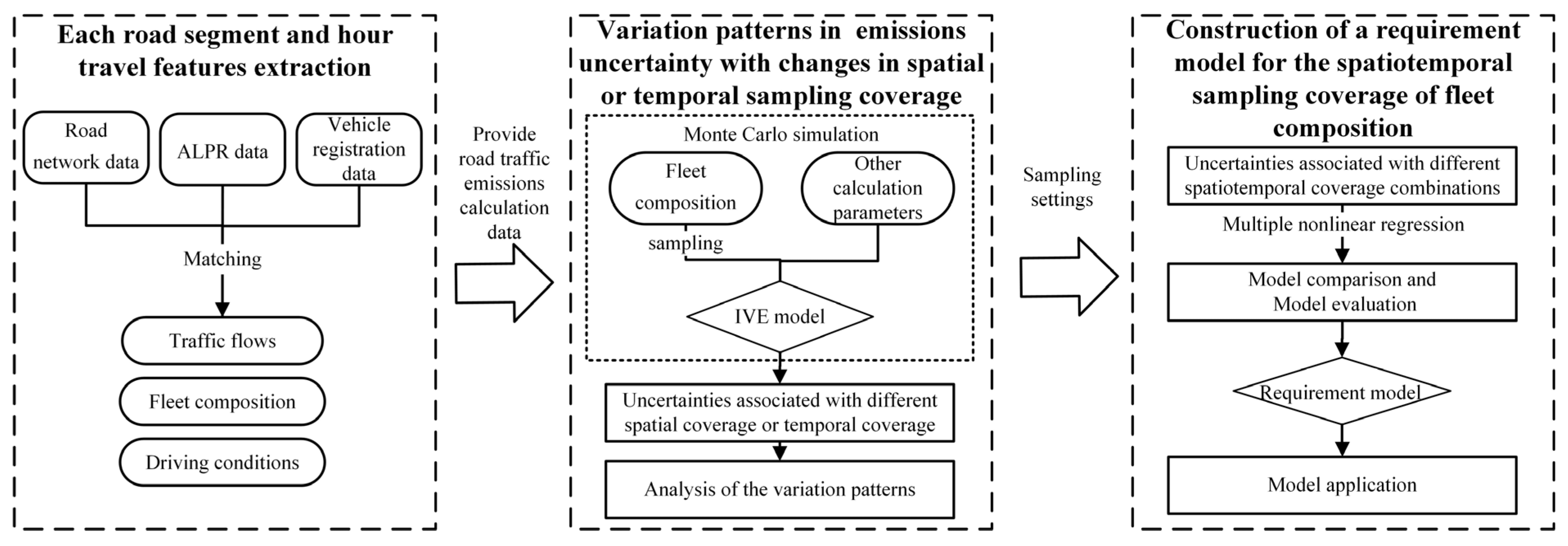
2. Materials and Methods

The overall research framework of this article is shown in Figure 1. (1) Using road network data, automatic licence plate recognition (ALPR) data, and vehicle registration data, this study acquired the parameters necessary for emissions calculations, such as traffic flows, fleet composition, and driving conditions, for each road segment and hour. (2) Using the IVE model and Monte Carlo simulation, this study calculated the uncertainties associated with regional daily road traffic emissions for different spatial or temporal coverage levels and then analysed the variation patterns in uncertainties. (3) This study calculated the uncertainties associated with different spatiotemporal coverage combinations of regional daily road traffic emissions, and constructed a requirement model for the spatiotemporal sampling coverage of fleet composition for the quantification of regional daily road traffic emissions.

2.1. Research Area and Data Sources

In this study, the core urban area of Xuancheng city was selected as the research area for the following reasons. First, Xuancheng is one of the 27 central cities in the Yangtze River Delta, a typical small and medium-sized city in China experiencing rapid development (see Figure S1). Its population in 2018 was 2.64 million. From 2005 to 2018, the per capita gross regional product (GDP) of Xuancheng grew at an annual rate of 10.5%. Cities of this size will play an important role in the construction of green cities in the future [24]. Second, the car ownership per capita in Xuancheng (0.15 vehicles/person) was close to the national average in China (0.166 vehicles/person) [25]. The fleet composition in the core urban area of Xuancheng was similar to that in other small and medium-sized Chinese cities, such as Langfang [26], Yangquan [27], and Foshan [28], with light passenger cars accounting for more than 85% of the total traffic mileage, while the proportions of heavy passenger cars, light-duty trucks, and heavy-duty trucks were relatively low at approximately 2%, 5%, and 2%, respectively. Therefore, the fleet composition in Xuancheng is highly representative of that of other small and medium-sized Chinese cities. Third, the urban core area is often congested and densely populated, thus increasing the health risks associated with traffic pollution. Fourth, the central area of Xuancheng was densely equipped with ALPR detectors, providing data samples with high spatiotemporal sampling coverage for this study. Through the ALPR detectors, traffic flow and licence plate information for vehicles on corresponding roads can be obtained, thereby further supporting accurate emissions and uncertainty quantification.

The road segments covered by ALPR detectors in the study area are shown in Figure 2, and include 113 monitored road segments categorized into expressways, arterial roads, and local roads [28], with each category accounting for approximately one-third of the total road length. The coverage of ALPR detectors on expressways and arterial roads within the area was nearly 100%. The urban structure of the study area exhibits a typical radial pattern [29].

The ALPR dataset in this study comprises approximately 40 million records obtained from 10 May to 9 June 2018. The types of data collected include the detector location ID, licence plate number, and detection time of each vehicle passing by a specific detector. Based on the aforementioned data, the traffic volume on each road segment every hour, the driving time of each vehicle in each segment, the average driving speed, etc., can be calculated. An example of the ALPR data is shown in

Table 1. Examples of ALPR data.

Record Number	Detector Location ID	Licence Plate Number (Anonymized)	Detection Time
1	HK-84	964352155	2018/5/8 07:00:05
2	HK-91	964352146	2018/5/8 07:30:55
3	HK-136	964352158	2018/5/8 08:20:50

.

By correlating ALPR data with licence plate numbers in the Xuancheng vehicle registration database, we can obtain detailed technical attribute information for vehicles travelling on each road segment every hour (further explained in the Section 2.2). Consequently, the fleet composition can be determined for each road segment every hour. Due to the lack of technical information on unregistered vehicles in the registration database and the fact that 90% of the traffic volume in the study area involves registered vehicles, this study primarily focuses on registered vehicles.

2.2. Emission Quantification Method

This study used the IVE model to calculate hourly segment-level emissions [30]. The IVE model, developed by the International Sustainable Systems Research Center (ISSRC) and University of California, Riverside (UCR), is known as an efficient tool for developing traffic emission inventories in developing countries [31] and has been widely used in China [29], India [21], and Iran [22]. The fleet composition of each hour and road segment was composed of the proportion of mileage travelled by each vehicle type to the total mileage [17], with the proportion calculation formula shown in Equation (1).

$$P_{t,h,l}=\frac{L_{t,h,l}}{L_{h,l}}=\frac{Q_{t,h,l} \times D_l}{Q_{h,l} \times D_l}$$

(1)

where P_t,h,l is the proportion of vehicle kilometres travelled (VKT) by vehicle type t on road segment l during hour h; L_t,h,l is the VKT of vehicle type t in road segment l during hour h, m; L_h,l is the VKT of all vehicles in road segment l during hour h, m; Q_t,h,l is the traffic volume of vehicle type t in road segment l during hour h, veh/h; Q_h,l is the traffic volume of road segment l during hour h, veh/h; and D_l is the length of road segment l, m.

The emissions from each hour and road segment are obtained by summing the emissions for each vehicle type, and the corresponding formula as shown in Equation (2). Regional emissions can be calculated by summing all road segments, and daily emissions can be calculated by summing the hourly emissions.

$$E_{h,l,j}={\sum }_t\frac{{\overline{V}}_{FTP} \times D_l \times { Q}_{h,l} \times P_{t,h,l} \times B_{t,j} \times K_{h,t,l,j}}{{\overline{V}}_{h,l}}$$

(2)

where E_h,l,j is the emissions of gas j on road segment l during hour h, g/h; ${\overline{V}}_{FTP}$ is average speed of the LA4 driving cycle, which is set to 8.7 m/s; B_t,j is the basic emission factor of emission j of vehicle type t, g/veh/km; K_h,t,l,j is other correction factors (speed correction, oil correction, etc.) for emission j of vehicle type t, g/veh/km; and ${\overline{V}}_{h,l}$ is the vehicle average driving speed of road segment l during hour h, m/s.

Vehicle types in the IVE model are categorized into over 1300 types based on various technical attributes, including description, weight, fuel type, exhaust characteristics, and age (defined by cumulative mileage). In this study, the method for matching each vehicle’s base emission factors and correction factors, based on vehicle registration data, refers to the approach described by Yu et al. [29]. The comparison and examples of vehicle technical information used in the IVE model and from the Xuancheng registration database are shown in

Table 2. Comparison and examples of vehicle technical information used in the IVE model and from the Xuancheng registration database.

Vehicle Technical Attribute Parameters in the IVE Model	Example of Vehicle Technical Attribute Parameters in the IVE Model	Corresponding Parameters in the Xuancheng Registration Database	Example of Xuancheng Registration Database
Weight	<2268 kg	Mass	2000 kg
Description	<1.5 L	Displacement	1 L
Fuel	Petrol	Fuel	Petrol
Exhaust	EURO I	Exhaust	China 1 1
Age	<79 × 106 m	Registration date, vehicle type and function	For detailed vehicle age estimation methods, please refer to Yu et al. [29]
Air/Fuel Control	Multi-Pt FI	-	Determined based on the vehicle’s Description and Exhaust
Evaporative	PCV/Tank	-	Determined based on the vehicle’s Description and Exhaust

¹ The emission standards are recorded as the China 1–5, which can be considered equal to the EURO I−V respectively [32].

.

This study focused on the uncertainty of NOx and CO₂ emissions because of their importance for air quality and climate change [33,34]. Furthermore, among common vehicle pollutants and greenhouse gases (VOC, CO, NOx, SO₂, and CO₂), the variability in emission factors among vehicle types for NOx and CO₂ was the largest and smallest, respectively. Therefore, analysing NOx and CO₂ aids in understanding the potential ranges and trends of uncertainties for common vehicle pollutants and greenhouse gases as sampling coverage changes.

2.3. Uncertainty Quantification Method

As regional daily total emissions are a key indicator involved in current emissions management policies, this research mainly focuses on the uncertainty of daily road traffic emissions at the regional level within the study area [35,36]. Uncertainty is a lack of knowledge of the true value of a variable and can be described with a confidence interval characterizing the range of possible values [37]. Current studies commonly use Monte Carlo simulations to calculate emission uncertainties [38,39,40]. In this study, the emission uncertainties associated with differences in spatiotemporal sampling coverages were calculated via Monte Carlo simulation.

To provide general guidance for the existing studies, the spatiotemporal sampling coverage was defined based on current research [17,18,19]. The specific examples are shown in Table S1. For temporal sampling, one hour was selected as the smallest sampling unit, and stratified sampling was conducted based on daytime and nighttime. For spatial sampling, given that fleet composition samples are typically obtained based on a certain number of road segments or intersections, a single road segment between two adjacent intersections was selected as the smallest sampling unit. Stratified spatial sampling was conducted based on road type (the road type was detailed in the Section 2.1). According to these settings, temporal sampling coverage refers to the proportion of sampled hours (e.g., 2 h) to the total number of hours (24 h in this study) representing the full period for emissions quantification. Spatial sampling coverage refers to the proportion of the number of sampled road segments to the total number of road segments in the study area.

The Monte Carlo method to calculate uncertainty for a specified spatiotemporal sampling coverage combination (which refers to sampling with a specific spatial coverage and temporal coverage) involves the following steps. First, T-fold random sampling simulations were performed. In this study, T was set to 1000 [41,42]. The sample size of each sampling simulation was determined based on the spatiotemporal sampling coverage and sampling population. Second, the fleet composition for the time periods and road segments included in the sample were calculated via Equation (1). Third, in each simulation, the fleet composition of hours and road segments not included in the sample were extrapolated based on the samples already collected, the calculation method is shown in Equation (3).

$$P_{t,h^{*},l^{*}}=\frac{{\sum }_{h,l}{L}_{t,h,l}}{{\sum }_{h,l}{L}_{h,l}}=\frac{{\sum }_{h,l}{Q}_{t,h,l} \times D_l}{{\sum }_{h,l}{Q}_{h,l} \times { D}_l}$$

(3)

where $P_{t,h^{*},l^{*}}$ is the proportion of VKT by vehicle type t on road segment l* during hour h*, inferred from the sample, l* refers to the road segment to be inferred, and h* refers to the hour period to be inferred.

Fourth, the regional daily road traffic emissions were calculated for this simulation via Equation (2). Finally, the emission calculation results from the 1000-fold simulations for a single spatiotemporal sampling coverage combination were used to compute a 95% confidence interval to represent uncertainties.

2.4. Method for Constructing the Requirement Model for the Spatiotemporal Sampling Coverage of Fleet Composition

The goal of this section was to develop a method to provide guidance for sampling fleet composition data for quantifying daily road traffic emissions in the core urban area. First, it was essential to determine the respective relationships of the temporal and spatial sampling coverages of fleet composition with the resulting uncertainties in emission quantification. Calculating uncertainties for all possible combinations of spatiotemporal coverage using Monte Carlo simulation requires substantial computational effort. Therefore, it is necessary to construct function models that approximates the relationship between spatiotemporal coverage and regional daily road traffic emission uncertainties based on a series of experiments. In each of these experiments, the uncertainties were measured for specified spatiotemporal coverage settings.

To effectively construct the function models, we first determined the patterns of uncertainty variations for different typical spatial sampling coverages (assuming that the temporal sampling coverage is constantly 100%) and for temporal sampling coverages (assuming that the spatial sampling coverage is constantly 100%) in sequence. The sample collection scheme was designed based on methods found in the current research [17,18,19], as presented in Table S1. Second, to intuitively reflect the patterns of variations, we fitted functions with emission uncertainties as the dependent variable and spatial/temporal sampling coverage as the independent variables. Third, for intervals of temporal or spatial sampling coverage in which the change in uncertainties was significant, the number of spatiotemporal sampling coverage combinations was increased to more effectively reflect these changes. Finally, based on the results of the uncertainties associated with different combinations of spatiotemporal sampling coverage, we constructed a model that delineated the relationship between assorted combinations of spatiotemporal sampling coverage and their resultant uncertainties. The selection of an appropriate fitting method for this model hinges on the pattern analysis of variations delineated in the second step of the aforementioned.

After the requirement model was constructed, the minimum spatiotemporal sampling coverage requirements can be determined by inputting the targeted uncertainties into the model. The required sample size can be obtained by multiplying the minimum spatiotemporal sampling coverage determined by the requirement model and the total population. If the sample size result was a noninteger, it should be rounded up to the nearest (higher) integer to adhere to the principle of conservatism.

Given the similarity of the fleet composition in the study area to that of other small and medium-sized cities in China (as detailed in the Section 2.1), the model constructed has a general degree of applicability in such cities.

3. Results and Discussion

3.1. Variation Patterns in Regional Daily Road Traffic Emission Uncertainties with Changes in Spatial Sampling Coverage

The uncertainty (expressed as 95% confidence intervals) quantification results of NOx and CO₂ emissions on weekdays and weekends under different spatial sampling coverage levels are shown in Figure 3. Considering the similarity in the distribution of uncertainties between weekdays and weekends, the discussion below was based on the corresponding average values. With a temporal sampling coverage of 100%, as the spatial coverage of the samples increased, the uncertainties gradually and monotonically decreased towards zero. For NOx, in the case of a spatial sampling coverage of 5%, the emission uncertainties were −36~52%. When the spatial sampling coverage increased to 35% and 70%, the uncertainties decreased to −14~15% and −5~5%, respectively. In contrast, the uncertainties of CO₂ for the same spatial sampling coverage were smaller than that of NOx; notably, at a spatial sampling coverage of 5%, the uncertainties were −3~4%.

The uncertainties of NOx emissions exceeded those of CO₂ emissions when considering the same spatial sampling coverage. This is because there are more significant variations in NOx emission factors among vehicle types than those for CO₂, and there are distinct differences in fleet composition among road segments. For example, for road Segments 1 and 2 in this study area (both expressways), the vehicle type with the highest NOx emission factor was the heavy-duty old-age (Vehicle age is defined by cumulative mileage; the cumulative mileage of old-age vehicles is <79 K km, that of young-age vehicles is 79–161 K km, and that of new-age vehicles is >161 K km [43]) vehicles using China III diesel (referred to as Type A), and that with the lowest was the light-duty new-age vehicles using China IV gasoline (referred to as Type B), with the former’s base emission factor being 136 times that of the latter [43]. Within Segment 1, the VKT proportions of Type A and Type B were 0.13% and 20%, respectively, while in Segment 2, they were 1.8% and 19%, respectively. Therefore, estimating the fleet composition of Segment 1 based on that of Segment 2 could result in an overestimation of the VKT proportion of Type A and an underestimation of the VKT proportion of Type B, thereby significantly overestimating the emissions for Segment 1 beyond the actual values. In contrast, the difference between the highest and lowest CO₂ emission factors for different vehicle types on road Segments 1 and 2 was only five times. This means that the impact of variations in fleet composition among segments on the emissions calculation has less effect on gases with small differences in vehicle emission factors than gases with large differences. Therefore, to achieve the same uncertainty goal, the spatial sampling coverage of gases with large emission factors differences between vehicle types needs to be larger than that of gases with small differences.

Additionally, as the spatial sampling coverage increased, the magnitude of change in the corresponding uncertainties gradually decreased. For instance, when the spatial sampling coverage increased from 5% to 20%, the upper bound of NOx uncertainty decreased by 27% points and the lower bound increased by 12% points. However, when spatial sampling coverage increased from 20% to 50%, the upper bound decreased by only 13% points, and the lower bound increased by only 10% points. This shows a trend that the benefit of reducing uncertainty diminishes as the spatial sampling coverage increases. Meanwhile, the uncertainties at low spatial sampling coverage showed significant asymmetry, with greater upper bound than the lower bound’s absolute value. This phenomenon was caused by the non-negative characteristics of emissions and the strong influence of outliers of fleet composition under low spatial sampling coverage. This asymmetry decreased as spatial sampling coverage increased, and starting at 35%, the absolute values of the upper and lower bounds were almost the same, differing by less than 0.5% points. Thus, with lower spatial sampling coverage, the degree of overestimation in emission quantification will be greater than that of underestimation. If the tolerance of overestimation of emission results is lower than that of underestimation, the spatial sampling coverage should be further improved.

3.2. Variation Patterns in Regional Daily Road Traffic Emission Uncertainties with Changes in Temporal Sampling Coverage

The uncertainty quantification results of NOx and CO₂ emissions on weekdays and weekends at different temporal sampling coverage levels are shown in Figure 4. The uncertainties distributions for weekdays and weekends were similar; thus, the discussion below was based on the corresponding average values. With 100% spatial sampling coverage, the overall trend was that the uncertainties gradually and monotonically decreased, approaching zero as the temporal sampling coverage increased. For NOx, at a temporal sampling coverage of 10%, the emission uncertainties were −22~25%. When the temporal sampling coverage increased to 25% and 60%, the uncertainties decreased to −13~15% and −5~5%. In contrast, the uncertainties of CO₂ at the same temporal sampling coverage were less than that of NOx, with uncertainties of −2~2% at a temporal sampling coverage of 10%.

The reason why NOx emission uncertainties significantly exceeded those of CO₂ at the same temporal sampling coverage was similar to the reasoning introduced in the Section 3.1. The fleet compositions from 08:00–09:00 and 13:00–14:00 were used as examples. During these periods, the vehicle type with the highest NOx emission factor was heavy-duty old-aged vehicles using China II diesel (referred to as Type C), and the vehicle type with the lowest NOx emission factor was light-duty new-aged vehicles using China IV gasoline (referred to as Type D), with the former’s base emission factor being 170 times that of the latter. From 08:00–09:00, the VKT proportions of Type C and Type D were 0.01% and 17%, respectively, whereas from 13:00–14:00, they were 0.05% and 16%, respectively. Consequently, inferring the 07:00–08:00 fleet composition from the 12:00–13:00 fleet composition could lead to overestimation and underestimation of the traffic activity for Type C and Type D vehicles, respectively. In contrast, the difference between the highest and lowest CO₂ emission factors for different vehicle types at 08:00–09:00 and 13:00–14:00 was only five times. This inference would lead to a significant overestimation of emissions from 08:00–09:00 compared to the actual values.

As the temporal sampling coverage increased, the magnitude of change in the corresponding uncertainties gradually decreased. For instance, as the temporal sampling coverage increased from 10% to 25%, the upper bound of NOx uncertainty decreased by 11% points, and the lower bound increased by 8% points. However, as the temporal sampling coverage increased from 25% to 50%, the reduction in the upper bound was only 7% points, and the increased in the lower bound was only 6% points. This reflects the fact that the benefit of reducing uncertainty diminishes over time as temporal sampling coverage increases. Moreover, at low temporal sampling coverage, the uncertainties exhibit noticeable asymmetry. This asymmetry diminishes with increasing temporal sampling coverage, becoming almost identical in absolute value from 50% onwards, with a mere difference of 0.5% points. This is due to the non-negative characteristics of emissions and the significant impact of outliers in fleet composition when temporal sampling coverage is low. Therefore, the degree of overestimating emission quantification results with low temporal sampling coverages will be greater. If the tolerance of overestimation of emission results is lower than that of underestimation, the temporal sampling coverages should be further improved.

These findings provide guidance for the construction of a requirement model for the spatiotemporal sampling coverage of fleet composition. The suggestion is to use more uncertainties data at lower, and less uncertainties data at higher sampling coverages. This approach ensures that the model accurately represents the range of change and asymmetry on the upper and lower bounds of confidence intervals of uncertainties.

3.3. Construction of a Requirement Model for the Spatiotemporal Sampling Coverage of Fleet Composition

According to the analysis detailed in the Section 3.1 and Section 3.2, the variance in the emission uncertainties between weekdays and weekends was small when considering identical temporal or spatial sampling coverages. Therefore, data from weekdays and weekends were simultaneously used to construct a requirement model for the spatiotemporal sampling coverage of fleet composition for regional daily road traffic emissions.

Due to the significant nonlinear relationships between uncertainties and temporal and spatial sampling coverages, this study employed multivariate nonlinear regression to construct a spatiotemporal sampling coverage requirement model. Multivariate nonlinear regression can flexibly model complex nonlinear relationships among variables, and offers an objective mathematical framework [44]. Owing to the significant variation and asymmetry in emission uncertainties at low spatiotemporal sampling coverages, three coverages below 30% and two above 30%, namely, spatial sampling coverages of 2%, 10%, 21%, 50%, and 79% and temporal sampling coverages of 8%, 16%, 25%, 50%, and 80%, respectively, were selected. This selection creates 25 different spatiotemporal coverage combinations for uncertainty calculation. The results of these calculations are shown in Table S2.

Based on the uncertainty calculations for 25 spatiotemporal sampling coverage combinations, the requirement model was constructed using polynomial functions in this study. To determine the order of the polynomial model, significance test indicators (F value and p value) and the Bayesian information criterion (BIC) method were used. Although the third-order model displayed the best performance for all indicators, it was nonmonotonic within the value range, which does not comply with the data distribution pattern shown in the Section 3.1 and Section 3.2. The significance test of the second-order model yielded an F value of 425, a p value < 0.0001, and a BIC of −344, yielding results with greater significance and a better fit than those of the first-order model. Therefore, a second-order polynomial was adopted as the regression model, as shown in Equation (4).

$$f\left(x_1,x_2\right)=\left\{\begin{array}{c}a\lg x_1+b\lg x_2+c\lg x_1^2+d\lg x_2^2+e\lg x_1{x}_{2 }+f x_1,x_2\in (0\%, 100\%)\\ 0 x_1,x_2=100\%\end{array}\right.$$

(4)

where f(x₁,x₂) is the upper or lower bound for the 95% confidence interval of uncertainty; x₁ and x₂ are the spatial and temporal sampling coverages, respectively; and a, b, c, d, e, and f are the coefficients of the terms in the polynomial. Since the relationships between f(x₁,x₂) and x₁ and x₂ are nonlinear, this study performed a logarithm transformation on x₁ and x₂, thereby enabling the model to capture the relationships between f(x₁,x₂) and x₁ and x₂ more accurately.

The normalized mean squared error (MSE) and correlation coefficient (R²) are adopted as criteria for evaluating the performance of the model. The MSE measures the average square difference between the experimental results and model predictions, with values closer to 0 indicating higher model precision. The R² measures the correlation between the experimental results and model predictions, with R² values greater than 0.9 generally indicating high accuracy. The results of the coefficients, R² values and MSE values as shown in

Table 3. Second-order models regression results and evaluation indicators.

f(x1,x2)	Coefficient						R2	MSE
	a	b	c	d	e	f
Upper bound of NOx uncertainty	−0.026	−0.024	0.281	0.194	−0.049	0.049	0.993	4.8 × 10−4
Lower bound of NOx uncertainty	0.215	0.078	−0.037	−0.085	0.102	−0.028	0.985	2.7 × 10−4
Upper bound of CO2 uncertainty	0.004	0.002	0.030	0.025	−0.005	0.005	0.986	8.4 × 10−6
Lower bound of CO2 uncertainty	0.013	0.008	−0.007	−0.005	0.005	−0.003	0.987	2.1 × 10−6

. The R² values of the second-order regression models were all greater than 0.985, and the MSE values were less than 5 × 10⁻⁴. To validate the models reliability, an additional ten sets of random spatiotemporal sampling coverage combinations and corresponding emission uncertainties were used to test the model [45], with R² > 0.93 and MSE < 0.0001. The aforementioned indicators suggested that the models have strong explanatory power and can accurately fit actual data.

The spatiotemporal sampling coverage requirements corresponding to different upper and lower bounds of NOx and CO₂ uncertainty predicted by the requirement model are shown in Figure 5. Each point on the contour lines reflects a combination of spatiotemporal sampling coverage at the same level of uncertainty. The spatial and temporal sampling coverages interact in such a way that increasing one can reduce the minimum requirement for the other. For instance, to maintain the upper bound of NOx uncertainty within 15%, the recommended spatiotemporal sampling coverage should be no less than 30% for temporal and 22% for spatial aspects. As the temporal sampling coverage increases to 35%, 45%, and 55%, the corresponding minimum spatial sampling coverages should be no less than 42%, 34%, and 31%, respectively. The contour lines were almost paralleled to the y-axis in the area when the spatial sampling coverage was low and the temporal sampling coverage was high. This phenomenon indicated that significant changes in temporal sampling coverage do not greatly affect uncertainties in this region. Taking the upper bound of NOx uncertainty as an example, when the spatial sampling coverage was 8% and the temporal sampling coverage was 33%, the upper bound was 50%. When only the temporal sampling coverage was increased to 100%, the upper bound decreased to 47%, a reduction of only 3% points. A similar phenomenon was also observed in areas with low temporal sampling coverage. This pattern indicated that compared to increasing only one type of coverage, the combined enhancement of both spatial and temporal sampling coverages can more effectively reduce uncertainty. The contour lines were densely distributed in areas of low spatial and temporal sampling coverages (coverage below 30%), indicating that the impact of spatiotemporal sampling coverage on uncertainties were significant in these areas. This phenomenon implied that enhancing sampling coverage in areas with initially low spatiotemporal density has a more significant impact on reducing uncertainty than in areas with already high coverage.

Researchers can determine the spatiotemporal sampling coverage corresponding to the upper and lower bounds of acceptable uncertainty for various gases and then select the most stringent spatiotemporal sampling coverage for fleet composition data. For example, to achieve the NOx uncertainties target of ±15%, the temporal and spatial sampling coverages corresponding to the upper and lower uncertainty bounds of +15% and −15%, respectively, were intersected. The results suggested that the recommended minimum temporal and spatial sampling coverages should be no less than 31% and 22%, respectively. The possible combinations of the least spatial and temporal sampling coverages included 43% and 36%, 34% and 45%, etc. Similarly, to achieve the CO₂ uncertainties target of ±3%, the recommended minimum temporal and spatial sampling coverages should be no less than 11% and 10%, respectively. The possible combinations of the least spatial and temporal sampling coverages included 17% and 16%, 15% and 18%, etc. These data showed that despite a lower uncertainties target for NOx compared to CO₂, calculating NOx emissions necessitated greater spatiotemporal sampling coverage due to higher variability in NOx emission factors among vehicle types. Based on these findings, it can be generalized that under the same uncertainties targets, gases with larger emission factor discrepancies among vehicle types, such as NOx, necessitate greater spatiotemporal sampling coverages than those required for gases with smaller discrepancies, such as CO₂. Therefore, sampling efforts should be prioritized for gases with larger emission factor discrepancies.

The framework and conclusions proposed in this study provide relevant insights on minimum threshold of spatiotemporal sampling coverage of fleet composition in calculating urban road traffic emissions, which assist in guiding fleet composition sampling, such as the development of manual sampling schemes and the installation of urban traffic cameras. Research conducted in urban areas similar to the case described in this work can employ the function models or the framework proposed in this work to obtain guidance on the spatiotemporal sampling coverage for fleet composition. These practices help avoid insufficient sampling and sampling that is excessively based on mere experience, thereby reducing uncertainty in emissions calculations. Moreover, emission data with reduced uncertainty can more accurately depict the severity and reduction potential of regional road traffic pollution and carbon emissions. These data thus support the selection of more precise and appropriate emission reduction measures.

The findings of this work are based on the use of IVE models in typical small and medium-sized Chinese city. Direct application of these results to studies in other types of urban areas or those employing different emission models may not yield accurate outcomes, especially in developed countries and large cities. Nevertheless, our generic framework lays a solid foundation for adaptation and application in diverse settings. Future research could apply this approach in various regions and with different models to test its relevance and adaptability, enhancing the robustness and utility of our findings in broader emission quantification efforts.

4. Conclusions

Given the absence of studies exploring the relationship between different spatiotem-poral sampling coverages of vehicle fleet composition and emission uncertainties, it was difficult to determine a reasonable spatiotemporal sampling coverage to accurately quantify regional daily road traffic emissions. In response to the aforementioned research gaps in existing studies, this study proposed a framework to manage uncertainty in urban road traffic emissions associated with vehicle fleet composition from the perspective of spatio-temporal sampling coverage. This study was conducted in the core urban area of Xuancheng, a typical small and medium-sized city in China, using the widely applied IVE model. Initially, the respective relationships of the temporal and spatial sampling cover-ages of fleet composition with the resulting regional daily road traffic emission uncertain-ties were determined. Subsequently, function models were developed to explore the determination of the spatiotemporal sampling coverage of fleet composition.

These results of emission uncertainties and function models implied that gases with larger emission factor discrepancies between vehicle types, such as NOx, required greater spatiotemporal sampling coverage than gases with smaller discrepancies, such as CO₂. Therefore, sampling efforts should be prioritized for gases with larger emission factor discrepancies. Additionally, increasing sampling coverage in one dimension (either spatial or temporal) can reduce the minimum required coverage in the other dimension. To achieve the NOx uncertainties target of ±15%, the recommended minimum temporal and spatial sampling coverages should be no less than 31% and 22%, respectively. The possible combinations of the least spatial and temporal sampling coverages included 43% and 36%, 34% and 45%, etc. To achieve the CO₂ uncertainties target of ±3%, the recommended minimum temporal and spatial sampling coverages should be no less than 11% and 10%, respectively. The possible combinations of the least spatial and temporal sampling coverages included 17% and 16%, 15% and 18%, etc. To further reduce uncertainty, enhancing both spatial and temporal sampling coverage of the fleet composition is more effective than enhancing one type of coverage alone.

This study provided a reference tool for determining the spatiotemporal sampling coverage of fleet composition for cities with similar fleet composition and vehicle scales. The tool aids in avoiding insufficient sampling, thereby reducing uncertainty in regional daily road traffic emission quantification. This reduction in uncertainty contributes to the development of more precise and effective emission reduction policies, ultimately leading to a reduction in greenhouse gas and air pollutant emissions from urban road traffic and fostering sustainable economic and social development.

References

1. Gao, C.; Gao, C.; Song, K.; Xing, Y.; Chen, W. Vehicle emissions inventory in high spatial–temporal resolution and emission reduction strategy in Harbin-Changchun Megalopolis. Process. Saf. Environ. Prot. 2020, 138, 236–245. [Google Scholar] [CrossRef]
2. Mendoza, D.; Gurney, K.R.; Geethakumar, S.; Chandrasekaran, V.; Zhou, Y.; Razlivanov, I. Implications of uncertainty on regional CO2 mitigation policies for the U.S. onroad sector based on a high-resolution emissions estimate. Energy Policy 2013, 55, 386–395. [Google Scholar] [CrossRef]
3. Khazini, L.; Kalajahi, M.J.; Blond, N. An analysis of emission reduction strategy for light and heavy-duty vehicles pollutions in high spatial–temporal resolution and emission. Environ. Sci. Pollut. Res. 2020, 29, 23419–23435. [Google Scholar] [CrossRef] [PubMed]
4. Chen, X.; Jiang, L.; Xia, Y.; Wang, L.; Ye, J.; Hou, T.; Zhang, Y.; Li, M.; Li, Z.; Song, Z.; et al. Quantifying on-road vehicle emissions during traffic congestion using updated emission factors of light-duty gasoline vehicles and real-world traffic monitoring big data. Sci. Total. Environ. 2022, 847, 157581. [Google Scholar] [CrossRef] [PubMed]
5. Gately, C.K.; Hutyra, L.R. Large uncertainties in urban-scale carbon emissions. J. Geophys. Res. Atmos. 2017, 122, 11242–11260. [Google Scholar] [CrossRef]
6. Viteri, R.; Borge, R.; Paredes, M.; Pérez, M.A. A high resolution vehicular emissions inventory for Ecuador using the IVE modelling system. Chemosphere 2023, 315, 137634. [Google Scholar] [CrossRef] [PubMed]
7. Ropkins, K.; Beebe, J.; Li, H.; Daham, B.; Tate, J.; Bell, M.; Andrews, G. Real-world vehicle exhaust emissions monitoring: Review and critical discussion. Crit. Rev. Environ. Sci. Technol. 2009, 39, 79–152. [Google Scholar] [CrossRef]
8. Shan, X.; Chen, X.; Jia, W.; Ye, J. Evaluating urban bus emission characteristics based on localized MOVES using sparse GPS data in Shanghai, China. Sustainability 2019, 11, 2936. [Google Scholar] [CrossRef]
9. Cai, H.; Xie, S.D. Determination of emission factors from motor vehicles under different emission standards in China. Acta Sci. Nat. Univ. Pekin. 2010, 46, 319–326. (In Chinese) [Google Scholar] [CrossRef]
10. Gamboa, J.R.; Pachón, J.E.; Leuro, O.M.C.; González, S.F. A new database of on-road vehicle emission factors for Colombia: A case study of Bogotá. CTyF Cienc. Tecnol. Futuro 2019, 9, 73–82. [Google Scholar] [CrossRef]
11. Zhang, Y.; Liu, Y.; Reng, P.P.; Yang, Z.; Yuan, Y.; Mao, H.; Andre, M. Research on vehicle activity characteristics of typical roads in Tianjin. Environ. Pollut. Control 2018, 40, 365–372. [Google Scholar] [CrossRef]
12. Cifuentes, F.; González, C.M.; Trejos, E.M.; López, L.D.; Sandoval, F.J.; Cuellar, O.A.; Mangones, S.C.; Rojas, N.Y.; Aristizábal, B.H. Comparison of top-down and bottom-up road transport emissions through high-resolution air quality modeling in a city of complex orography. Atmosphere 2021, 12, 1372. [Google Scholar] [CrossRef]
13. Li, R.; Yang, F.; Liu, Z.; Shang, P.; Wang, H. Effect of taxis on emissions and fuel consumption in a city based on license plate recognition data: A case study in Nanning, China. J. Clean. Prod. 2019, 215, 913–925. [Google Scholar] [CrossRef]
14. Yang, N.; Yang, L.; Xu, F.; Han, X.; Liu, B.; Zheng, N.; Li, Y.; Bai, Y.; Li, L.; Wang, J. Vehicle emission changes in China under different control measures over past two decades. Sustainability 2022, 14, 16367. [Google Scholar] [CrossRef]
15. Dias, D.; Amorim, J.H.; Sá, E.; Borrego, C.; Fontes, T.; Fernandes, P.; Pereira, S.R.; Bandeira, J.; Coelho, M.C.; Tchepel, O. Assessing the importance of transportation activity data for urban emission inventories. Transp. Res. Part D Transp. Environ. 2018, 62, 27–35. [Google Scholar] [CrossRef]
16. Gong, M.; Yin, S.; Gu, X.; Xu, Y.; Jiang, N.; Zhang, R. Refined 2013-based vehicle emission inventory and its spatial and temporal characteristics in Zhengzhou, China. Sci. Total. Environ. 2017, 599, 1149–1159. [Google Scholar] [CrossRef] [PubMed]
17. Sun, D.; Zhang, K.; Shen, S. Analyzing spatiotemporal traffic line source emissions based on massive didi online car-hailing service data. Transp. Res. Part D Transp. Environ. 2018, 62, 699–714. [Google Scholar] [CrossRef]
18. Meng, X.; Zhang, K.; Pang, K.; Xiang, X. Characterization of spatio-temporal distribution of vehicle emissions using web-based real-time traffic data. Sci. Total. Environ. 2020, 709, 136227. [Google Scholar] [CrossRef]
19. Li, X.; Lopes, D.; Mok, K.M.; Miranda, A.I.; Yuen, K.V.; Hoi, K.I. Development of a road traffic emission inventory with high spatial–temporal resolution in the world’s most densely populated region—Macau. Environ. Monit. Assess. 2019, 191, 239. [Google Scholar] [CrossRef] [PubMed]
20. Li, N.; Gao, C.; Ba, Q.; You, H.; Zhang, X. Towards sustainable transport: Quantifying and mitigating pollutant emissions from heavy-duty diesel trucks in Northeast China. Environ. Sci. Pollut. Res. 2023, 30, 119518–119531. [Google Scholar] [CrossRef] [PubMed]
21. Mishra, D.; Goyal, P. Estimation of vehicular emissions using dynamic emission factors: A case study of Delhi, India. Atmospheric Environ. 2014, 98, 1–7. [Google Scholar] [CrossRef]
22. Shafabakhsh, G.; Taghizadeh, S.A.; Kooshki, S.M. Investigation and sensitivity analysis of air pollution caused by road transportation at signalized intersections using IVE model in Iran. Eur. Transp. Res. Rev. 2018, 10, 7. [Google Scholar] [CrossRef]
23. Liu, Z.; Liu, S.; Qi, W.; Jin, H. Urban sprawl among Chinese cities of different population sizes. Habitat Int. 2018, 79, 89–98. [Google Scholar] [CrossRef]
24. Central Committee of the Communist Party of China. State Council. Outline of Regional Integration Development Plan for the Yangtze River Delta. Available online: https://www.gov.cn/zhengce/2019-12/01/content_5457442.htm (accessed on 15 March 2024).
25. National Bureau of Statistics, P.R.C. China Statistical Yearbook 2019; China Statistics Press: Beijing, China, 2019. [Google Scholar]
26. Sun, S.; Jin, J.; Xia, M.; Liu, Y.; Gao, M.; Zou, C.; Wang, T.; Lin, Y.; Wu, L.; Mao, H.; et al. Vehicle emissions in a middle-sized city of China: Current status and future trends. Environ. Int. 2020, 137, 105514. [Google Scholar] [CrossRef] [PubMed]
27. Xie, S.X.; Huang, Z.H.; Wang, X.; Tang, W.X.; He, W.N.; Ji, L.; Wang, Y.J.; Ni, H. Emission inventory of motor vehicle based on traffic flow for Yangquan City in 2017. J. Environ. Eng. Technol. 2021, 11, 226–233. (In Chinese) [Google Scholar] [CrossRef]
28. Liu, Y.H.; Ma, J.L.; Li, L.; Lin, X.-F.; Xu, W.-J.; Ding, H. A high temporal-spatial vehicle emission inventory based on detailed hourly traffic data in a medium-sized city of China. Environ. Pollut. 2018, 236, 324–333. [Google Scholar] [CrossRef] [PubMed]
29. Yu, Z.; Li, W.; Liu, Y.; Zeng, X.; Zhao, Y.; Chen, K.; Zou, B.; He, J. Quantification and management of urban traffic emissions based on individual vehicle data. J. Clean. Prod. 2021, 328, 129386. [Google Scholar] [CrossRef]
30. Ghaffarpasand, O.; Talaie, M.R.; Ahmadikia, H.; Khozani, A.T.; Shalamzari, M.D. A high-resolution spatial and temporal on-road vehicle emission inventory in an Iranian metropolitan area, Isfahan, based on detailed hourly traffic data. Atmos. Pollut. Res. 2019, 11, 1598–1609. [Google Scholar] [CrossRef]
31. Mohammadiha, A.; Malakooti, H.; Esfahanian, V. Development of reduction scenarios for criteria air pollutants emission in Tehran Traffic Sector, Iran. Sci. Total. Environ. 2018, 622, 17–28. [Google Scholar] [CrossRef] [PubMed]
32. Jing, B.; Wu, L.; Mao, H.; Gong, S.; He, J.; Zou, C.; Song, G.; Li, X.; Wu, Z. Development of a vehicle emission inventory with high temporal–spatial resolution based on NRT traffic data and its impact on air pollution in Beijing—Part 1: Development and evaluation of vehicle emission inventory. Atmos. Meas. Tech. 2016, 16, 3161–3170. [Google Scholar] [CrossRef]
33. Ministry of Ecology and Environment of China. Bulletin of the Second National Pollution Source Census. Available online: https://www.gov.cn/xinwen/2020-06/10/content_5518391.htm (accessed on 15 March 2024).
34. Li, Y.; Bao, L.; Li, W.; Deng, H. Inventory and policy reduction potential of greenhouse gas and pollutant emissions of road transportation industry in China. Sustainability 2016, 8, 1218. [Google Scholar] [CrossRef]
35. Ministry of Environmental Protection. Technical regulation on Ambient Air Quality Index (AQI) (Trial). Available online: https://www.mee.gov.cn/ywgz/fgbz/bz/bzwb/jcffbz/201203/W020120410332725219541.pdf (accessed on 15 March 2024).
36. State General Administration of Quality Supervision, Inspection and Quarantine, Ministry of Environmental Protection. Ambient Air Quality Standard. Available online: https://www.mee.gov.cn/ywgz/fgbz/bz/bzwb/dqhjbh/dqhjzlbz/201203/W020120410330232398521.pdf (accessed on 15 March 2024).
37. IPCC. 2006 IPCC Guidelines for National Greenhouse Gas Inventories. Chapter 3 Uncertainties; Institute for Global Environmental Strategies (IGES): Hayama, Japan, 2006; p. 8. [Google Scholar]
38. Muthén, L.K.; Muthén, B.O. How to use a monte carlo study to decide on sample size and determine power. Struct. Equ. Model. A Multidiscip. J. 2002, 9, 599–620. [Google Scholar] [CrossRef]
39. Zhang, Z.; Song, G.; Zhai, Z.; Li, C.; Wu, Y. How many trajectories are needed to develop facility- and speed-specific vehicle-specific power distributions for emission estimation? Case study in Beijing. Transp. Res. Rec. J. Transp. Res. Board 2019, 2673, 779–790. [Google Scholar] [CrossRef]
40. Chen, Y.; Zhang, Y.; Borken-Kleefeld, J. When is enough? Minimum sample sizes for on-road measurements of car emissions. Environ. Sci. Technol. 2019, 53, 13284–13292. [Google Scholar] [CrossRef] [PubMed]
41. Beasley, W.H.; Rodgers, J.L. Bootstrapping and Monte Carlo methods. In APA Handbook of Research Methods in Psychology; American Psychological Association: Washington, DC, USA, 2012; Volume 2, pp. 407–425. [Google Scholar]
42. Qumsiyeh, M. Using the bootstrap for estimating the sample size in statistical experiments. J. Mod. Appl. Stat. Methods 2013, 12, 45–53. [Google Scholar] [CrossRef]
43. ISSRC. IVE Model User’s Manual Version 2.0. Available online: https://manualzilla.com/doc/5821819/ive-model-users-manual-international-sustainable-systems (accessed on 15 March 2024).
44. Zhang, K.; Li, W.; Han, Y.; Geng, Z.; Chu, C. Production capacity identification and analysis using novel multivariate nonlinear regression: Application to resource optimization of industrial processes. J. Clean. Prod. 2021, 282, 124469. [Google Scholar] [CrossRef]
45. Mäkelä, M. Experimental design and response surface methodology in energy applications: A tutorial review. Energy Convers. Manag. 2017, 151, 630–664. [Google Scholar] [CrossRef]
Figure 1. Research framework.
Sustainability 16 03504 g001
Figure 2. The location and road network of the study area in this paper.
Sustainability 16 03504 g002
Figure 3. At different spatial sampling coverage levels, the uncertainties of NOx (a) and CO2 (b) emissions on weekdays and weekends.
Sustainability 16 03504 g003
Figure 4. At different temporal sampling coverage levels, the uncertainties of NOx (a) and CO2 (b) emissions on weekdays and weekends.
Sustainability 16 03504 g004
Figure 5. Contour plots of spatial and temporal sampling coverages with upper and lower bounds of NOx (a) and CO2 (b) uncertainty.
Sustainability 16 03504 g005