

Influence of Regional Temperature Anomalies on Strawberry Yield: A Study Using Multivariate Copula Analysis

1
Department of Systems Design Engineering, University of Waterloo, Waterloo, ON N2L 3G1, Canada
2
Department of Electrical & Computer Engineering, University of Waterloo, Waterloo, ON N2L 3G1, Canada
3
Department of Machine Learning, Mohamed bin Zayed University of Artificial Intelligence, Masdar City, Abu Dhabi 50819, United Arab Emirates
*
Authors to whom correspondence should be addressed.
Sustainability 2024, 16(9), 3523; https://doi.org/10.3390/su16093523
Submission received: 25 March 2024
/
Revised: 11 April 2024
/
Accepted: 18 April 2024
/
Published: 23 April 2024
(This article belongs to the Special Issue Sustainability of Agriculture: The Impact of Climate Change on Crops)
Abstract
:A thorough understanding of the impact of climatic factors on agricultural production is crucial for improving crop models and enhancing predictability of crop prices and yields. Fluctuations in crop yield and price can have significant implications for the market sector and farming community. Given the projected increase in frequency and intensity of extreme events, reliable modelling of cropping patterns becomes essential. Temperature anomalies are expected to play a prominent role in future extreme events, emphasizing the need to comprehend their influence on crop yield. Forecasting extreme yield, which encompasses both the highest and lowest levels of agricultural production within a given time period, along with peak crop prices representing the highest market values, poses greater challenges in forecasting compared to other values. Probability-based predictions, accounting for uncertainty and variability, offer a more accurate approach for extreme value estimation and risk assessment. In this study, we employ a multivariate analysis based on vine copula to explore the interdependencies between temperature anomalies and daily strawberry yield in Santa Maria, California. By considering the maximum and minimum daily yields each month, we observe an increased probability of yield loss with rising temperature anomalies. While we do not explicitly consider the specific impacts of temperature anomalies under individual Representative Concentration Pathway (RCP) scenarios, our analysis is conducted within the broader context of the current global warming scenario. This allows us to capture the overall anticipated effects of regional temperature anomalies on agriculture. The findings of this study have potential impacts and consequences for understanding the vulnerability of agricultural systems and improving crop model predictions. By enhancing our understanding of the relationships between temperature anomalies and crop yield, we can inform decision-making processes related to the impact of climate change on agriculture. This research contributes to the ongoing efforts in improving agricultural sustainability and resilience in the face of changing climatic conditions.
1. Introduction
Agricultural production is highly sensitive to climatic variabilities [1,2,3]. The recurrence of extreme events such as heat waves, droughts, flood, etc., are pushing the global crop productivity to an extremely vulnerable state and this will have a profound impact on food security [2,4]. Among the climatic factors influencing crop yield, temperature anomalies are most likely to influence the crop yields negatively [4,5,6,7,8] and can ultimately impact a crop’s market values. Considering the current climate change crisis, quantifying the impact of temperature anomalies on crop yields will be of significant value in planning adaptive strategies to assist agriculture and to avoid risk of food insecurity. The response of crops to high temperature stress has been studied in detail for different crops such as groundnut, wheat, maize, and rice, most of them involving experimental studies [9,10,11,12,13,14].
Temperatures that lie outside the range of optimum temperature levels for crops can have severe repercussions on the irrigated crop yields [15]. Both high and low temperatures can create a distress in the rate of agricultural production [4,16]. Understanding crop productivity responses to the regional weather and their explicit inclusion in crop models will aid in improving the planning of agricultural production.
Over the past few years, significant progress has been made in understanding the climate–yield relationships by many researchers. For instance, Goulart et al., 2021 [17] used a random forest model and global warming scenarios to predict an increase in soybean crop failures in the Midwestern United States due to warmer summer conditions. They introduced the concept of impact-analogues, which are expected to increase with warmer climates, providing a comprehensive risk estimation of future scenarios. Zhang et al., 2023 [18] examined the impact of climate extremes on vegetation growth on the Tibetan Plateau, utilizing event coincidence analysis to assess the susceptibility of different vegetation types to drought, extreme wet, hot, and cold events. They highlighted the importance of understanding vegetation responses to climate variability and identified ecologically sensitive regions that may be at risk due to changing climate conditions. Feng et al., 2021 [19] examined the evolving relationship between climate variables and crop yield, highlighting the impact of concurrent changes in precipitation–yield and temperature–yield relationships on the risk of crop yield reduction. They proposed a statistical approach to assess these risks, especially under compound dry–hot conditions, and underscored the importance of adapting agricultural planning to these changing climate–yield dynamics. Powell et al., 2015 [20] examined the impact of extreme weather events on wheat yields in the Netherlands, utilizing econometric techniques on farm-level panel data and established a correlation between increased frequency of such events and reduced yields, highlighting the importance of local-level analysis for accurate measurement and forecasting. Shayanmehr et al., 2020 [21] examined the impact of climate change on potato yield and variability in Iran’s Agro-Ecological Zones (AEZs) for the 2050s, using models to project local climate scenarios and assess future agricultural outcomes. They highlighted the need for region-specific strategies to mitigate yield reduction and ensure food security in the face of changing climatic conditions.
Some of the previous similar studies focus on the influence of isolated extreme events such as heat waves and droughts on crop yields [22,23]. Recent studies have shown that the concurrent weather extremes can create larger impacts to the crop yield than isolated extreme events [19,24].
While different crop models and AI models were able to predict the non-extreme yield and price of strawberry and other crops with reasonable accuracy, the accurate prediction of extreme (both maximum and minimum) yield and price is found to be difficult [25,26]. However, these extreme yields are highly important in quantifying the profits for different stakeholders such as farmers and the market sector. Identifying the interdependence of extreme values in the crop sector can play a crucial role in improving the extreme value prediction performance of models. An integrated, probabilistic model by incorporating the uncertainties and interdependencies between the crop yield and weather anomalies can improve the prediction of crop yield, especially the extreme values [27].
This study focuses on analyzing the variations in strawberry yield in relation to the anomalies in regional air temperature within the study area in California, United States. Strawberry is a lucrative farm produce and has a critically low shelf life. Currently, the market for strawberries alone is worth USD 3.02 billion and they are one of the top ten most valued commodities for California and the United States’ economy [28].
Strawberries reach maturity and bear fruit relatively quickly due to their shallow root systems, necessitating optimal light conditions for high yield and fruit quality. Additionally, proper water management is essential to maximize both yield and fruit quality in strawberries [29]. With an aim of explaining the influence of regional weather conditions on strawberries, several studies have been carried out [29,30,31]. Some of these studies have shown a critical correlation between strawberry yield and temperature changes [29,30,32]. Temperature affects nutrient uptake and photosynthesis in strawberry plants [33]. High temperature can also inhibit developmental stages during flower formation and can eventually bog down the fruit quality [34].
In our study, we made a deliberate choice to primarily focus on temperature anomalies as the key climatic factor influencing crop yield. This decision is supported by compelling justifications based on the unique characteristics of the study area and the current irrigation practices used to grow this commercial crop. Firstly, the area is characterized by strict irrigation practices, where crop growth and yield are predominantly reliant on controlled water supply rather than natural precipitation. This reduces the impact of variations in precipitation on crop yield [35], making temperature anomalies one of the primary climatic factors of interest. While soil moisture is undoubtedly crucial for crop growth and development, strict irrigation practices in the study area ensure that soil moisture levels are maintained at optimal levels, minimizing their variability and impact on crop yield. Additionally, extensive analysis of historical data revealed a strong and consistent correlation between temperature anomalies and crop yield in the study area. In contrast, the correlation between precipitation and yield was found to be comparatively weaker and hence is not reported here. This finding highlights the dominant role of temperature anomalies in driving yield variations, underscoring the need to investigate and understand their impact for improved agricultural predictions.
Furthermore, our choice to focus on temperature anomalies aligns with previous studies conducted in similar agricultural contexts. Existing research consistently highlights the significant influence of temperature fluctuations on crop growth, development, and yield potential [36,37,38]. By emphasizing temperature anomalies, we build upon this knowledge and contribute to the growing understanding of their impact on agricultural systems. Considering the expected temperature rise and its potential consequences for agricultural production [39], understanding the influence of temperature anomalies becomes crucial. Higher temperatures can have profound effects on critical physiological processes in crops, such as photosynthesis, respiration [39], and water use efficiency [36]. By focusing on temperature anomalies, we aim to uncover the specific interdependencies between temperature variations and crop performance, contributing to the development of more robust and accurate agricultural models and predictions. Here, we present a data-based analysis of the influence of temperature anomalies on the extreme strawberry yield over the Southwestern United States. This study here is trying to analyze and figure out the importance of extreme value analyses. A multivariate copula analysis has been used to understand the conditional probability of decreasing yield given the temperature anomalies. Understanding of the influence of temperature anomalies on crop yield will help in the development of appropriate adaptation measures for agriculture planning and management. The findings of this work help in understanding responses of strawberry extreme yields to the regional temperature anomalies, which is critical to address the needs of the farming communities and to help the agricultural marketing industry in making appropriate price predictions.
2. Materials and Methods
2.1. Data
In this study, the strawberry yield from Santa Maria County in California, United States, was analyzed with respect to the regional air temperature anomalies. California holds significant importance in the global strawberry industry, being responsible for producing over 80% of the fresh market and processed strawberries grown in the United States. Moreover, it accounts for approximately 20% of the world’s total strawberry production [40]. The Central Coast and Santa Maria Valley of California collectively host two-thirds of the total acreage dedicated to strawberry production [28,40].
Growers in the Santa Maria region have historically employed drip irrigation systems. In the Santa Maria Valley, strawberry fields are typically divided into drip-irrigated sections ranging from 1 to 5 acres. The drip lines used have lengths varying between 200 and 325 feet, with high-flow, 4 mil drip tape featuring emitters spaced every 8 inches and installed at depths of 1 to 3 inches. Additionally, drip tapes are replaced annually to ensure optimal irrigation efficiency [41]. Furthermore, to address concerns regarding the representativeness of monitored meteorological conditions, it is important to note that the cultivation practices described herein are widely adopted across the entire region [41]. This ensures that temperature data collected accurately reflect the prevailing environmental conditions experienced by strawberry crops in the Santa Maria Valley.
The study period spans from 2011 to 2019, capturing a comprehensive dataset of strawberry yield variations in the Santa Maria Valley. It is pertinent to note that throughout the study period, consistent irrigation practices were maintained, with minimal deviations observed. This ensures the reliability of yield data and allows for a more accurate assessment of the impact of temperature anomalies on strawberry yield dynamics.
The daily data of strawberry yield and temperature pertaining to Santa Maria County in California for a time period from 2011 to 2019 were collected from two publicly available websites [42,43]. In this study, the influence of temperature anomalies on the strawberry yields was analyzed. For this purpose, the monthly maximum temperature anomalies were estimated as the deviations from the average monthly temperature from 1991 to 2021 that is publicly available on the website [44].
In order to define the yield loss with respect to the daily strawberry yield extremes, the following guidelines were proposed in this study.
The standardised yield was estimated by standardizing the maximum and minimum daily yield over each month by means of z score transformation as given below.
where Std. Ymax and Std. Ymin are the standardised daily maximum and minimum yield over each month, Ymax and Ymin are the maximum and minimum daily yield over each month, and are the mean of the maximum and minimum yield time series data (for every month in the time period), and and are the standard deviation of the maximum and minimum yield time series data.
In this study, for better understanding, the yield loss is defined as three types of losses (low, moderate, and high). The three categories of yield loss are defined in this study as follows:
The monthly temperature anomalies were analyzed with the standardised maximum and minimum strawberry yield at Santa Maria for the time period from 2011 to 2019.
2.2. Copula Analysis
Sklar [45] first introduced copula in 1959. Copulas are largely useful in describing the dependencies between random variables [46]. They are mathematical functions by which we can obtain a joint distribution of random variables using their univariate distributions. The major utility of copulas comes where the random variables under consideration do not follow the same marginal distributions in which case it is difficult to find joint distribution without the use of a copula.
Sklar’s theorem states that for a given joint multivariate distribution function and relevant marginal distributions for the corresponding random variables, there always exists a copula function that relates the marginal distributions of the variables [45] which can be mathematically derived as follows:
Consider the bivariate case with two random variables, X1 and X2, with distribution functions F1(X1) and F2(X2), respectively. As per Sklar’s theorem there always exists a copula function (C) such that,
where C(ul,u2) is itself a distribution function where u1 and u2 are F1(x1), F2(x2)), respectively.
F(X1 = x1, X2 = x2) = C(F1(x1), F2(x2))
A copula can be described as a cumulative distribution function with a uniform marginal. Each of the marginal distributions produces a probability of events. The copula function maps these probabilities to a joint probability, by giving a relationship on the probabilities. Hence, copulas build multivariate distributions by merely determining the dependence between the random variables without having any influence on the marginals. The detailed mathematical formulations and derivations of copulas can be seen in many scientific articles [47,48,49]
In contrast to bivariate copulas, which are very popular in various fields such as finance, marketing, hydrology [50,51,52,53,54], etc., applicability of multivariate copulas was seldom explored until recently due to the complexity in the construction of multivariate copulas. Vine copula is a flexible multi-variate copula construction method [49,55,56] which has a large potential for many multi-variate data analysis applications. The underlying theory for the vine copula is from Joe [57]. The use of vine copulas is gaining popularity in various fields [58,59,60,61,62,63].
2.3. Construction of a 3-Dimensional Vine Copula
The selection of the copula function that best describes the given data is a crucial step in the analysis of data using copulas. In the current study, the focus will be on a 3-dimensional vine copula coupling the three marginal distributions of three random variables, X, Y and Z (monthly maximum yield, monthly minimum yield, and monthly temperature anomaly). We assume that the samples of all three variables were each transformed (U, V, and W) so that all three variables are now approximately uniformly distributed on [0, 1]. The fundamental idea of vine copulas is to construct multivariate copulas based on a hierarchical mixing of bivariate copulas [64]. All pairwise dependencies are modelled with bivariate copulas. If all mutual dependencies defined are with respect to the same variable, the construction is called a canonical vine (C-vine). If all mutual dependences are considered one after the other variable, this is called a D-vine [65]. C- and D-vines are special cases of regular vines.
Fitting a C-vine might be advantageous when a particular variable is known to be a key variable that governs interactions in the data set. In such a case, this variable can be placed at the root of the canonical vine structure [66]. Different vine copula decompositions produce different multivariate distributions [65]. The selection of the vine copula structure is an important stage in the modelling process, which can be performed by any of the available methods in the literature such as based on the absolute empirical Kendall tau [67], and maximum likelihood method [66]. Here, the maximum likelihood method is used, by considering different copula families and the best fit is determined by the highest log-likelihood value. The estimations in this paper were performed using R 4.2.2, which is an open-source software environment for statistical computing, and the package “VineCopula” [68].
2.4. Calculation of Joint Probability of Occurrence of Events Using Copula
The major focus of this study is to understand the dependency of standardised strawberry yields (both maximum and minimum) on temperature anomaly. A 3D copula is used in this study and the joint probabilities of occurrence of strawberry yield and temperature anomalies for various scenarios are estimated. Different combinations of relations with the fitted copula distribution and the marginal distributions can be used to estimate the joint probabilities of occurrence of events. Some of which, those that were used in this study, are given below:
2.4.1. Univariate Probability
Univariate probability denotes the probability of an event by considering the marginal distribution of the random variable alone. The mutual dependencies of the variable with other random variables are not considered here. This type of probability will be referred to as UP in this paper from here onwards.
where F is the cumulative distribution function of the random variable (X).
UP(X ≤ x) = F(x)
UP(X > x) = 1 − F(x)
2.4.2. Joint Probability for Tri-Variate Events
In multivariate frequency analysis involving three variables using copula, the following probability distributions can be used where C is the copula function.
For tri-variate random variables, X1, X2, and X3, some of the formulae of tri-variate probability distributions is given as follows [49]:
2.4.3. Conditional Probability of Tri-Variate Events
For tri-variate random variables, X1, X2, and X3, the conditional probability of occurrence of events can be estimated with the help of the underlying copulas. An example case is defined below [49]:
Case 1:
In this case, under the condition , both values of and are exceeded. In this case:
where
More detailed mathematical expressions can be found in Zhang and Singh [49].
3. Preliminary Data Analysis
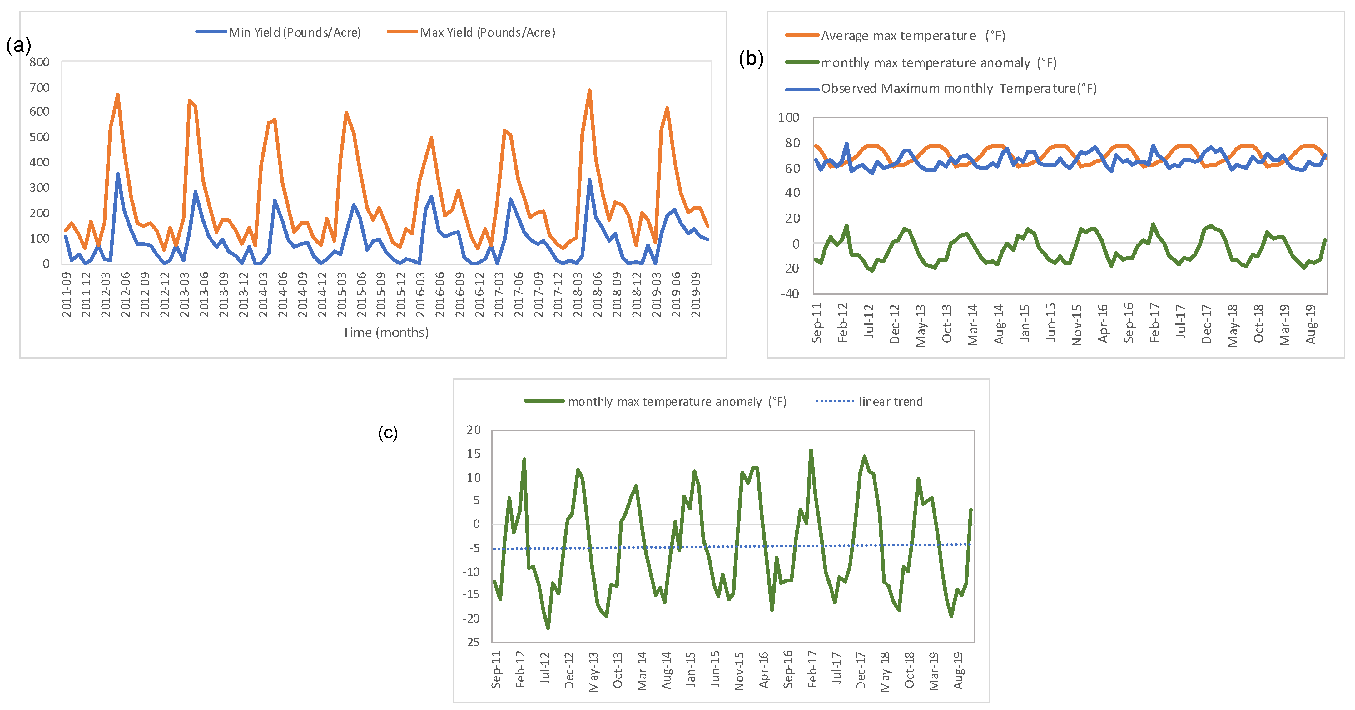
Before starting any modelling process, it is always advisable to carry out a preliminary data analysis. The primary focus of this study is on strawberry yield affected by temperature anomalies. Hence, the maximum and minimum daily yield over each month have been estimated and are given in Figure 1a. It can be observed that the yield data are an approximately stationary process with a predominant seasonal pattern with peak yield during June. Similarly, the maximum monthly temperature observed at Santa Maria from 2011 to 2019 and the average maximum temperature over months based on temperature data from 1990 to 2021 [44] are given in Figure 1b. The monthly maximum temperature anomalies are estimated by calculating the deviation of the observed maximum temperature from the average maximum temperature over months and are shown in Figure 1b,c. As the data length is comparatively short to estimate long-term trends in the data, the temperature anomaly does not show any predominant trend (Figure 1c). It can be inferred that the yield and the temperature anomaly data are approximate stationary processes during the time period of 2011–2019. The basic statistics of the data are given in Table 1.
4. Results and Discussion
In order to identify the correlation of strawberry yield and the temperature anomaly, a 3D copula analysis was carried out with standardised maximum and minimum daily strawberry yield over each month and monthly maximum temperature anomaly as the three random variables. To conduct multi-variate copula analysis, a vine copula structure was selected for this study. Apart from a multivariate analysis, individual univariate frequency analyses of the random variables were also conducted to identify the relevance of using copula analysis in conducting analysis of dependent random variables.
4.1. Univariate Analysis
As the first case, univariate frequency analysis of the random variables is conducted without considering the interdependence between the random variables. The random variables (standardised maximum yield, standardised minimum yield, and the temperature anomaly) were analyzed individually. The histograms of the variables are given in Figure 2. It can be observed from the histograms that the standardised maximum and minimum yields are positively skewed whereas the temperature anomalies show both skewness and heavy tails.
Different probability distributions were tested and the marginal probability distribution that describes the process best was selected for each of the random variables. The “GAMLSS” [69,70] package in R was used for the purpose. Skew exponential power type III (SEP3) distribution was found to be the best fit for standardised maximum and minimum yield data whereas skewed exponential power type II (SEP2) distribution was found to best describe the temperature anomaly process.
Hence, the identified univariate probability distributions for the three variables were fitted to the data. From the marginal distribution, the probability of different cases (events) as described in Equation (3) were calculated using Equations (5) and (6) and are tabulated, which is given in Table 2.
As the standardised maximum and minimum yields follow the same marginal distribution (SEP3), their joint probability can be found by directly applying the product rule for independent events as follows:
4.2. Multivariate Copula Analysis Using Vine Copula
We employed vine copulas also known as pair-copula constructions (PCC) to model the dependence of strawberry yield and temperature anomaly. To model the dependence using vine copula, the data from the real domain were transformed to copula data, such that all data points lie inside [0, 1]. This was accomplished by computing the pseudo-observations of the data matrix by weighing the original variables based on the covariance structure of the data. The use of pseudo-observations helps to retain the essential structure of the data while making it easier to fit statistical models and interpret the results. Working with the pseudo-observations eliminates the marginal properties of the variables and retains the information about their interdependence [71].
The root node of a C-vine tree is identified by identifying the node with the strongest dependencies to all other nodes. The node with the maximum column sum in the empirical Kendall’s tau matrix is selected as the root node. To do this, the Kendall correlation matrix for the variables was generated and the absolute value of the correlation coefficient of each variable was added together (Table 3). The variable with the highest sum is selected as the root node of the C-vine tree. In our case study, the root node of the C-vine tree is the minimum strawberry yield. The vine tree structure selected for this study is given in Figure 3.
We used bivariate copulas to formulate the PCC for the three links. Each link represents a bivariate copula that best describes the dependence between the corresponding variables. The bivariate copulas selected for each of the links are also shown in Figure 3. The selection and fitting of the copula were performed in R 4.2.2 using the “VineCopula” package. Copulas are fitted against the data using maximum likelihood estimation, and then the Akaike information criteria (AIC) criterion is computed for different copula families in R package “VineCopula” [68]. The Tawn II copula (asymmetric logistic copula) [72,73] which is an extension of the Gumbel copula describes the dependence of the marginal distributions of standardised minimum yield and standardised maximum yield. BB8 (Joe−Frank) copula, which is a mixture model of the Joe and Frank copulas, describes the relation between standardised minimum yield and temperature anomaly, and the Joe copula describes the conditional relation with standardised maximum yield and temperature anomaly given standardised minimum yield.
Based on the fitted copula, the standardised maximum strawberry yield, standardised minimum strawberry yield, and temperature anomaly were simulated and compared with the observed data (Figure 4). It was observed that the copula could capture the pattern and behaviour of the yield and temperature data.
The joint probability analysis of standardised minimum and maximum strawberry yield and temperature anomaly was conducted using a vine copula. The focus of this study was to determine the impact of temperature anomaly on strawberry yield through conditional probability analysis. The conditional probability (CP) of standardised minimum and maximum strawberry yield (as given in Equation (3)) given the temperature anomaly was analyzed using the established vine copula. The results of the scenarios analyzed are presented in Table 4, which displays the conditional probability of various yield loss conditions for different temperature anomalies.
Table 4 demonstrates the impact of temperature anomalies on the standardised minimum and maximum strawberry yields. The table shows the probability of yield loss events (with its severity) for different temperature anomaly conditions. Our findings clearly demonstrate that temperature anomalies have a significant impact on strawberry yield in Santa Maria, California. By comparing the univariate and multivariate analysis results (as shown in Table 2 and Table 4), we highlight the significance of multivariate probabilistic analysis in crop yield studies. The univariate analysis (Table 2), which focuses solely on marginal distributions, tends to underestimate the likelihood of yield loss events. This oversight occurs because it overlooks the intricate relationship between temperature anomalies and crop yields.
In contrast, the multivariate copula analysis, incorporating the joint dependence structure, allows for a more accurate assessment of the conditional probabilities of yield loss events for different temperature anomalies. This approach captures the interdependencies between temperature anomalies and crop yield, revealing the complex relationship between the variables. By considering the joint dependence structure, our analysis reveals that the conditional probability of various yield loss events is much higher for different possible temperature anomalies. For instance, we observe that when the temperature anomaly exceeds 3 °F, high yield loss events are highly probable. This highlights the critical importance of considering the intricate relationship between temperature anomalies and crop yields.
This comparison between the univariate and multivariate analyses underscores the importance of considering multivariate dependencies when studying the effects of temperature anomalies on crop yield, particularly in the context of climate change. Thus, copula-based multivariate analysis offers valuable insights by capturing the joint dependence structure between variables, enabling a more realistic assessment of the risks associated with temperature anomalies.
This study highlights the importance of understanding the influence of temperature anomalies on extreme crop yields and estimating the risk of yield reduction under extreme weather conditions to ensure food security under global warming. By applying copula analysis, we can accurately assess conditional probabilities and gain detailed insights into the influence of temperature anomalies on crop yields. It offers a more realistic assessment of the risks associated with temperature anomalies, enabling stakeholders to devise more effective risk management and climate change adaptation strategies. This becomes particularly relevant in the current climate change scenario, where global warming is projected and understanding the impact of temperature anomalies on agricultural production becomes crucial for effective adaptation and decision making. By understanding the complex relationship between temperature anomalies and crop yields, stakeholders can implement targeted measures to minimize yield losses and enhance the resilience of agricultural systems in the face of climate change.
The results of this study will be helpful in developing an integrated probabilistic crop climate model with improved prediction performance, especially in predicting the extreme crop yields and prices. The implications of our findings are significant for strawberry farmers in Santa Maria, California. Understanding the dependency patterns between temperature anomalies and crop yield can inform farmers about the risks associated with temperature extremes and help them make informed decisions regarding crop management practices, irrigation scheduling, and other adaptation measures. This knowledge can guide farmers and policymakers in implementing effective climate change adaptation strategies in strawberry production and potentially in other high-value agricultural crops.
5. Limitations of This Study
Despite the valuable insights gained from our study, it is important to acknowledge its limitations. These limitations include the following:
Generalizability: The findings of our study are specific to the context of Santa Maria, California, and the strawberry crop. Extrapolating these results to other regions or agricultural crops should be done with caution, as different crops and regions may exhibit unique climatic and agronomic characteristics. A significant area of future research could be exploring the potential compounding effects of extreme heat and drought on crops, especially in rain-fed regions, by considering other climate variables.
Biotic factors: In the current study, we considered commercial fully irrigated (pest controlled) crops, hence the influence of biotic factors, such as diseases, on crop yield was not explicitly considered in our analysis. Incorporating biotic variables into the copula modelling framework is a potential avenue for future research to improve the comprehensiveness of yield predictions especially for noncommercially grown crops.
Time scale: Another limitation of our study is the relatively short time scale of the research data, which ranges from 2011 to 2019. A longer time scale, ideally spanning at least 30 years, would be more suitable for studying the relationship between crop yield and climate change. This limitation should be acknowledged as it may affect the generalizability of our findings to longer-term climate variations. As future research, expanding the time frame can be considered, which will enhance our understanding of the changing climate–crop dynamics.
Despite these limitations, this study offers a valuable tool for analyzing the influence of temperature anomalies on strawberry yield. It provides a framework for studying the complex dependencies between climate variables and crop performance. Our results contribute to the growing understanding of climate–crop relationships and demonstrate the potential for utilizing multivariate copula analysis in agricultural decision making and climate change adaptation.
6. Conclusions
This study utilizes C-vine copula analysis to investigate the relationship between temperature anomalies and strawberry yield in Santa Maria, California. The findings demonstrate a significant dependence between temperature anomalies and crop yield, highlighting the importance of considering temperature variations in crop climate models.
While our study illustrates the influence of temperature on crop yield, integrating such analysis into broader crop models can yield more actionable insights for agricultural production practices. Such integrated models hold practical implications, offering guidance for decision-making processes aimed at mitigating the effects of temperature anomalies on crop production and contributing to the broader knowledge base on climate and agriculture. By incorporating temperature anomalies into crop models, resource allocation can be optimized, crop yield predictions can be improved, and farming system resilience can be enhanced.
This research contributes to the broader understanding of the intricate relationships between regional temperature anomalies and agricultural outcomes. By employing multivariate copula analysis, we showcase its effectiveness in quantifying the dependence between temperature anomalies and crop yield.
Future research can expand on our findings by including additional factors such as biotic factors and applying copula analysis to other high-value agricultural crops. This would further refine the predictive capabilities of crop climate models and provide a comprehensive understanding of temperature anomalies’ impact on different agricultural systems.
Author Contributions
Conceptualization, P.U. and K.P.; methodology, P.U.; software, P.U.; validation, P.U., K.P. and F.K.; formal analysis, P.U.; investigation, P.U.; resources, P.U.; data curation, P.U.; writing—original draft preparation, P.U.; writing—review and editing, P.U., K.P. and F.K.; visualization, P.U.; supervision, K.P. and F.K.; project administration, P.U.; funding acquisition, K.P. and F.K. All authors have read and agreed to the published version of the manuscript.
Funding
This research was partially funded by NSERC and Loblaws NSERC-CRD.
Data Availability Statement
The raw data supporting the conclusions of this article will be made available by the authors on request.
Conflicts of Interest
The authors declare no conflict of interest.
References
- Kumari, A.; Lakshmi, G.A.; Krishna, G.K.; Patni, B.; Prakash, S.; Bhattacharyya, M.; Singh, S.K.; Verma, K.K. Climate Change and Its Impact on Crops: A Comprehensive Investigation for Sustainable Agriculture. Agronomy 2022, 12, 3008. [Google Scholar] [CrossRef]
- Elias, E.H.; Flynn, R.; Idowu, O.J.; Reyes, J.; Sanogo, S.; Schutte, B.J.; Smith, R.; Steele, C.; Sutherland, C. Crop Vulnerability to Weather and Climate Risk: Analysis of Interacting Systems and Adaptation Efficacy for Sustainable Crop Production. Sustainability 2019, 11, 6619. [Google Scholar] [CrossRef]
- Malhi, G.S.; Kaur, M.; Kaushik, P. Impact of Climate Change on Agriculture and Its Mitigation Strategies: A Review. Sustainability 2021, 13, 1318. [Google Scholar] [CrossRef]
- Talib, M.N.A.; Ahmed, M.; Naseer, M.M.; Slusarczyk, B.; Popp, J. The Long-Run Impacts of Temperature and Rainfall on Agricultural Growth in Sub-Saharan Africa. Sustainability 2021, 13, 595. [Google Scholar] [CrossRef]
- Eck, M.A.; Murray, A.R.; Ward, A.R.; Konrad, C.E. Influence of Growing Season Temperature and Precipitation Anomalies on Crop Yield in the Southeastern United States. Agric. For. Meteorol. 2020, 291, 108053. [Google Scholar] [CrossRef]
- John, R.P.; Megan, G. Temperatures and the Growth and Development of Wheat: A Review. Eur. J. Agron. 1999, 10, 23–36. [Google Scholar]
- Ottman, M.J.; Kimball, B.A.; White, J.W.; Wall, G.W. Wheat Growth Response to Increased Temperature from Varied Planting Dates and Supplemental Infrared Heating. Agron. J. 2012, 104, 7–16. [Google Scholar] [CrossRef]
- Zhao, C.; Liu, B.; Piao, S.; Wang, X.; Lobell, D.B.; Huang, Y.; Huang, M.; Yao, Y.; Bassu, S.; Ciais, P.; et al. Temperature Increase Reduces Global Yields of Major Crops in Four Independent Estimates. Proc. Natl. Acad. Sci. USA 2017, 114, 9326–9331. [Google Scholar] [CrossRef]
- Asseng, S.; Ewert, F.; Martre, P.; Rötter, R.P.; Lobell, D.B.; Cammarano, D.; Kimball, B.A.; Ottman, M.J.; Wall, G.W.; White, J.W.; et al. Rising Temperatures Reduce Global Wheat Production. Nat. Clim. Chang. 2015, 5, 143–147. [Google Scholar] [CrossRef]
- Challinor, A.J.; Wheeler, T.R.; Craufurd, P.Q.; Slingo, J.M. Simulation of the Impact of High Temperature Stress on Annual Crop Yields. Agric. For. Meteorol. 2005, 135, 180–189. [Google Scholar] [CrossRef]
- Ferris, R.; Ellis, R.H.; Wheeler, T.R.; Hadley, P. Effect of High Temperature Stress at Anthesis on Grain Yield and Biomass of Field-Grown Crops of Wheat. Ann. Bot. 1998, 82, 631–639. [Google Scholar] [CrossRef]
- Matsui, T.; Omasa, K.; Horie, T. The Difference in Sterility Due to High Temperatures during the Flowering Period among Japonica-Rice Varieties. Plant Prod. Sci. 2001, 4, 90–93. [Google Scholar] [CrossRef]
- Vara Prasad, P.V.; Craufurd, P.Q.; Summerfield, R.J.; Wheeler, T.R. Effects of Short Episodes of Heat Stress on Flower Production and Fruit-set of Groundnut (Arachis hypogaea L.). J. Exp. Bot. 2000, 51, 777–784. [Google Scholar] [CrossRef] [PubMed]
- Wang, X.; Peng, L.; Zhang, X.; Yin, G.; Zhao, C.; Piao, S. Divergence of Climate Impacts on Maize Yield in Northeast China. Agric. Ecosyst. Environ. 2014, 196, 51–58. [Google Scholar] [CrossRef]
- Karimzadeh Soureshjani, H.; Ghorbani Dehkordi, A.; Bahador, M. Temperature Effect on Yield of Winter and Spring Irrigated Crops. Agric. For. Meteorol. 2019, 279, 107664. [Google Scholar] [CrossRef]
- Grace, J. Temperature as a Determinant of Plant Productivity. Symp. Soc. Exp. Biol. 1988, 42, 91–107. [Google Scholar] [PubMed]
- Goulart, H.M.D.; van der Wiel, K.; Folberth, C.; Balkovic, J.; van den Hurk, B. Storylines of Weather-Induced Crop Failure Events under Climate Change. Earth Syst. Dyn. 2021, 12, 1503–1527. [Google Scholar] [CrossRef]
- Zhang, Y.; Hong, S.; Liu, D.; Piao, S. Susceptibility of Vegetation Low-Growth to Climate Extremes on Tibetan Plateau. Agric For Meteorol. 2023, 331, 109323. [Google Scholar] [CrossRef]
- Feng, S.; Hao, Z.; Zhang, X.; Hao, F. Changes in Climate-Crop Yield Relationships Affect Risks of Crop Yield Reduction. Agric. For. Meteorol. 2021, 304–305, 108401. [Google Scholar] [CrossRef]
- Powell, J.P.; Reinhard, S. Measuring the Effects of Extreme Weather Events on Yields. Weather Clim. Extrem. 2015, 12, 69–79. [Google Scholar] [CrossRef]
- Shayanmehr, S.; Rastegari Henneberry, S.; Sabouhi Sabouni, M.; Shahnoushi Foroushani, N. Climate Change and Sustainability of Crop Yield in Dry Regions Food Insecurity. Sustainability 2020, 12, 9890. [Google Scholar] [CrossRef]
- Schmitt, J.; Offermann, F.; Söder, M.; Frühauf, C.; Finger, R. Extreme Weather Events Cause Significant Crop Yield Losses at the Farm Level in German Agriculture. Food Policy 2022, 112, 102359. [Google Scholar] [CrossRef]
- Zipper, S.C.; Qiu, J.; Kucharik, C.J. Drought Effects on US Maize and Soybean Production: Spatiotemporal Patterns and Historical Changes. Environ. Res. Lett. 2016, 11, 094021. [Google Scholar] [CrossRef]
- Toreti, A.; Cronie, O.; Zampieri, M. Concurrent Climate Extremes in the Key Wheat Producing Regions of the World. Sci Rep 2019, 9, 5493. [Google Scholar] [CrossRef]
- Lobell, D.B.; Cahill, K.N.; Field, C.B. Weather-Based Yield Forecasts Developed for 12 California Crops. Calif. Agric. 2006, 60, 211–215. [Google Scholar] [CrossRef]
- Nassar, L.; Okwuchi, I.E.; Saad, M.; Karray, F.; Ponnambalam, K.; Agrawal, P. Prediction of Strawberry Yield and Farm Price Utilizing Deep Learning. In Proceedings of the 2020 International Joint Conference on Neural Networks (IJCNN), Glasgow, UK, 19–24 July 2020; IEEE: Piscataway, NJ, USA, 2020; pp. 1–7. [Google Scholar]
- Newlands, N.K.; Zamar, D.S.; Kouadio, L.A.; Zhang, Y.; Chipanshi, A.; Potgieter, A.; Toure, S.; Hill, H.S.J. An Integrated, Probabilistic Model for Improved Seasonal Forecasting of Agricultural Crop Yield under Environmental Uncertainty. Front. Environ. Sci. 2014, 2, 17. [Google Scholar] [CrossRef]
- California Department of Food and Agriculture (CDFA)—Statistics. Available online: https://www.cdfa.ca.gov/statistics/ (accessed on 9 October 2022).
- Li, H.; Li, T.; Gordon, R.J.; Asiedu, S.K.; Hu, K. Strawberry Plant Fruiting Efficiency and Its Correlation with Solar Irradiance, Temperature and Reflectance Water Index Variation. Environ. Exp. Bot. 2010, 68, 165–174. [Google Scholar] [CrossRef]
- Palencia, P.; Martínez, F.; Medina, J.J.; López-Medina, J. Strawberry Yield Efficiency and Its Correlation with Temperature and Solar Radiation. Hortic. Bras. 2013, 31, 93–99. [Google Scholar] [CrossRef]
- Waister, P.D. Wind as a Limitation on the Growth and Yield of Strawberries. J. Hortic. Sci. 1972, 47, 411–418. [Google Scholar] [CrossRef]
- Casierra-Posada, F.; Peña-Olmos, J.E.; Ulrichs, C. Basic Growth Analysis in Strawberry Plants (Fragaria sp.) Exposed to Different Radiation Environments. Agron. Colomb. 2012, 30, 25–33. [Google Scholar]
- Ganmore-Neumann, R.; Kafkafi, U. The Effect of Root Temperature and Nitrate/Ammonium Ratio on Straw-berry Plants. II. Nitrogen Uptake, Mineral Ions, and Carboxylate Concentrations. Agron J. 1985, 77, 835–840. [Google Scholar] [CrossRef]
- Heide, O.M. Photoperiod and Temperature Interactions in Growth and Flowering of Strawberry. Physiol. Plant. 1977, 40, 21–26. [Google Scholar] [CrossRef]
- Webber, H.; Ewert, F.; Olesen, J.E.; Müller, C.; Fronzek, S.; Ruane, A.C.; Bourgault, M.; Martre, P.; Ababaei, B.; Bindi, M.; et al. Diverging Importance of Drought Stress for Maize and Winter Wheat in Europe. Nat. Commun. 2018, 9, 4249. [Google Scholar] [CrossRef] [PubMed]
- Asseng, S.; Foster, I.; Turner, N.C. The Impact of Temperature Variability on Wheat Yields. Glob. Chang. Biol. 2011, 17, 997–1012. [Google Scholar] [CrossRef]
- Zabel, F.; Müller, C.; Elliott, J.; Minoli, S.; Jägermeyr, J.; Schneider, J.M.; Franke, J.A.; Moyer, E.; Dury, M.; Francois, L.; et al. Large Potential for Crop Production Adaptation Depends on Available Future Varieties. Glob. Chang. Biol. 2021, 27, 3870–3882. [Google Scholar] [CrossRef] [PubMed]
- Wang, Z.; Zhang, T.Q.; Tan, C.S.; Xue, L.; Bukovsky, M.; Qi, Z.M. Modeling Impacts of Climate Change on Crop Yield and Phosphorus Loss in a Subsurface Drained Field of Lake Erie Region, Canada. Agric. Syst. 2021, 190, 103110. [Google Scholar] [CrossRef]
- Eyshi Rezaei, E.; Webber, H.; Gaiser, T.; Naab, J.; Ewert, F. Heat Stress in Cereals: Mechanisms and Modelling. Eur. J. Agron. 2015, 64, 98–113. [Google Scholar] [CrossRef]
- United States Department of Agriculture. National Agricultural Statistics Service. Available online: https://www.nass.usda.gov/ (accessed on 9 April 2024).
- Hanson, B.; Bendixen, W. Drip Irrigation Evaluated in Santa Maria Valley Strawberries. Calif. Agric. 2004, 58, 48–53. [Google Scholar] [CrossRef]
- The California Strawberry Commission. Available online: https://www.calstrawberry.com/en-us/ (accessed on 9 January 2022).
- The California Irrigation Management Information System. Available online: http://www.cimis.water.ca.gov/ (accessed on 10 January 2022).
- Santa Maria Climate. Available online: https://en.climate-data.org/north-america/united-states-of-america/california/santa-maria-1488/ (accessed on 7 June 2022).
- Sklar, A. Fonctions de Repartition à n Dimensionls et Leurs Marges; Publications de l’Institut Statistique de l’Université de Paris: Paris, France, 1959; pp. 229–231. [Google Scholar]
- Ponnambalam, K.; Seifi, A.; Vlach, J. Yield Optimization with Correlated Design Parameters and Non-Symmetrical Marginal Distributions. In Proceedings of the 2003 International Symposium on Circuits and Systems, ISCAS ’03, Bangkok, Thailand, 25–28 May 2003; IEEE: Piscataway, NJ, USA, 2020; Volume 4, pp. IV-736–IV-739. [Google Scholar]
- Hofert, M.; Kojadinovic, I.; Machler, M.; Yan, J. Elements of Copula Modeling with R; Springer: Berlin/Heidelberg, Germany, 2018; ISBN 9783319896342. [Google Scholar]
- Nelson, R.B. An Introduction to Copulas, 2nd ed.; Bickel, P., Diggle, P., Fienberg, S., Gather, U., Olkin, I., Zeger, S., Eds.; Springer: Berlin/Heidelberg, Germany, 2006; ISBN 13:978-0387-28659-4. [Google Scholar]
- Zhang, L.; Singh, V.P. Copulas and Their Applications in Water Resources Engineering; Cambridge University Press: Cambridge, UK, 2019; ISBN 9781108565103. [Google Scholar]
- Latif, S.; Mustafa, F. Bivariate Flood Distribution Analysis under Parametric Copula Framework: A Case Study for Kelantan River Basin in Malaysia. Acta Geophys. 2020, 68, 821–859. [Google Scholar] [CrossRef]
- Roch, O.; Alegre, A. Testing the Bivariate Distribution of Daily Equity Returns Using Copulas. An Application to the Spanish Stock Market. Comput. Stat. Data Anal. 2006, 51, 1312–1329. [Google Scholar] [CrossRef]
- Vaz de Melo Mendes, B.; Mendes Semeraro, M.; Câmara Leal, R.P. Pair-Copulas Modeling in Finance. Financ. Mark. Portf. Manag. 2010, 24, 193–213. [Google Scholar] [CrossRef]
- Righi, M.B.; Ceretta, P.S. Analyzing the Dependence Structure of Various Sectors in the Brazilian Market: A Pair Copula Construction Approach. Econ. Model 2013, 35, 199–206. [Google Scholar] [CrossRef]
- Hu, L. Dependence Patterns Across Financial Markets: A Mixed Copula Approach. Appl. Financ. Econ. 2006, 16, 717–729. [Google Scholar] [CrossRef]
- Okhrin, O.; Ristig, A.; Xu, Y.-F. Copulae in High Dimensions: An Introduction. In Applied Quantitative Finance; Härdle, W., Chen, C.H., Overbeck, L., Eds.; Springer: Berlin/Heidelberg, Germany, 2017; ISBN 9783662544860. [Google Scholar]
- Zhang, M.; Bedford, T. Vine Copula Approximation: A Generic Method for Coping with Conditional Dependence. Stat. Comput. 2018, 28, 219–237. [Google Scholar] [CrossRef]
- Joe, H. Multivariate Models and Multivariate Dependence Concepts; Chapman and Hall/CRC: Boca Raton, FL, USA, 1997; ISBN 9780367803896. [Google Scholar]
- Nazir, H.M.; Hussain, I.; Faisal, M.; Mohamd Shoukry, A.; Abdel Wahab Sharkawy, M.; Fawzi Al-Deek, F.; Ismail, M. Dependence Structure Analysis of Multisite River Inflow Data Using Vine Copula-CEEMDAN Based Hybrid Model. PeerJ 2020, 8, e10285. [Google Scholar] [CrossRef] [PubMed]
- Spanhel, F.; Kurz, M.S. Simplified Vine Copula Models: Approximations Based on the Simplifying Assumption. Electron. J. Stat. 2019, 13, 1254–1291. [Google Scholar] [CrossRef]
- Latif, S.; Mustafa, F. Parametric Vine Copula Construction for Flood Analysis for Kelantan River Basin in Malaysia. Civ. Eng. J. 2020, 6, 1470–1491. [Google Scholar] [CrossRef]
- El Hannoun, W.; el Adlouni, S.-E.; Zoglat, A. Vine-Copula-Based Quantile Regression for Cascade Reservoirs Management. Water 2021, 13, 964. [Google Scholar] [CrossRef]
- Xu, P.; Wang, D.; Wang, Y.; Singh, V.P. A Stepwise and Dynamic C-Vine Copula–Based Approach for Nonstationary Monthly Streamflow Forecasts. J. Hydrol. Eng. 2022, 27, 04021043. [Google Scholar] [CrossRef]
- Chen, L.; Singh, V.P.; Shenglian, G.; Hao, Z.; Li, T. Flood Coincidence Risk Analysis Using Multivariate Copula Functions. J. Hydrol. Eng. 2012, 17, 742–755. [Google Scholar] [CrossRef]
- Bedford, T.; Cooke, R.M. Vines: A New Graphical Model for Dependent Random Variables. Ann. Stat. 2002, 30, 1031–1068. [Google Scholar] [CrossRef]
- Gräler, B.; van den Berg, M.J.; Vandenberghe, S.; Petroselli, A.; Grimaldi, S.; de Baets, B.; Verhoest, N.E.C. Multivariate Return Periods in Hydrology: A Critical and Practical Review Focusing on Synthetic Design Hydrograph Estimation. Hydrol. Earth Syst. Sci. 2013, 17, 1281–1296. [Google Scholar] [CrossRef]
- Aas, K.; Czado, C.; Frigessi, A.; Bakken, H. Pair-Copula Constructions of Multiple Dependence. Insur. Math. Econ. 2009, 44, 182–198. [Google Scholar] [CrossRef]
- Dißmann, J.; Brechmann, E.C.; Czado, C.; Kurowicka, D. Selecting and Estimating Regular Vine Copulae and Application to Financial Returns. Comput. Stat. Data Anal. 2013, 59, 52–69. [Google Scholar] [CrossRef]
- Nagler, T.; Schepsmeier, U.; Stoeber, J.; Brechmann, E.C.; Graeler, B.; Erhardt, T. VineCopula: Statistical Inference of Vine Copulas. Available online: https://github.com/tnagler/VineCopula (accessed on 11 January 2022).
- Rigby, R.; Stasinopoulos, M.; Heller, G.; De Bastiani, F. Distributions for Modelling Location, Scale and Shape: Using GAMLSS in R; CRC Press: Boca Raton, FL, USA, 2019. [Google Scholar]
- Stasinopoulos, D.M.; Rigby, R.A. Generalized Additive Models for Location Scale and Shape (GAMLSS) in R. J. Stat. Softw. 2007, 23, 1–46. [Google Scholar] [CrossRef]
- Jane, R.; Dalla Valle, L.; Simmonds, D.; Raby, A. A Copula-Based Approach for the Estimation of Wave Height Records Through Spatial Correlation. Coast. Eng. 2016, 117, 1–18. [Google Scholar] [CrossRef]
- Eschenburg, P. Properties of Extreme-Value Copulas; Universitat Munchen: München, Germany, 2013. [Google Scholar]
- Tawn, J.A. Bivariate Extreme Value Theory: Models and Estimation. Biometrika 1988, 75, 397–415. [Google Scholar] [CrossRef]
Figure 1.
(a) Maximum and minimum monthly strawberry yield at Santa Maria from 2011 to 2019; (b) the observed temperature at Santa Maria from 2011 to 2019 and the temperature anomalies estimated; (c) trend of monthly maximum temperature anomalies observed from 2011 to 2019.
Figure 1.
(a) Maximum and minimum monthly strawberry yield at Santa Maria from 2011 to 2019; (b) the observed temperature at Santa Maria from 2011 to 2019 and the temperature anomalies estimated; (c) trend of monthly maximum temperature anomalies observed from 2011 to 2019.

Figure 2.
Histogram of (a) standardised maximum strawberry yield at Santa Maria; (b) standardised minimum strawberry yield at Santa Maria; (c) temperature anomaly at Santa Maria for each month.
Figure 2.
Histogram of (a) standardised maximum strawberry yield at Santa Maria; (b) standardised minimum strawberry yield at Santa Maria; (c) temperature anomaly at Santa Maria for each month.

Figure 3.
C-Vine tree structure showing the dependencies and pair-copula structure.

Figure 4.
The standardised maximum and minimum strawberry yield and temperature anomaly along with the corresponding simulated data using the fitted copula.
Figure 4.
The standardised maximum and minimum strawberry yield and temperature anomaly along with the corresponding simulated data using the fitted copula.


Table 1.
Basic statistics of the yield and temperature anomaly data.
| Statistics | Max Yield (Pounds/Acre) | Min Yield (Pounds/Acre) | Max Temp Anomaly (°F) |
|---|---|---|---|
| Min. | 57.94 | 1 | −11.9 |
| 1st Qu. | 128.5 | 17.72 | −2.6 |
| Median | 185 | 73.74 | 4.5 |
| Mean | 245.66 | 86.21 | 5.839 |
| 3rd Qu | 327.67 | 123.15 | 13.85 |
| Max. | 686 | 356.32 | 25.9 |
Table 2.
Probability of the yield loss events and temperature anomaly (TA) to be more than the given thresholds using the univariate probability distribution of the random variables.
Table 2.
Probability of the yield loss events and temperature anomaly (TA) to be more than the given thresholds using the univariate probability distribution of the random variables.
| Events | Probability of Occurrence | Remarks |
|---|---|---|
| Std. Ymax , Std. Ymin | 0.004 | Yield loss |
| Std. Ymax , Std. Ymin | 0.0001 | Moderate or high yield loss |
| Std. Ymax , Std. Ymin | 0.25 × 10⁻⁶ | High yield loss |
| TA TA | 0.036 | Temperature anomaly is between the range of 1 °F and 2 °F |
| TA TA | 0.042 | Temperature anomaly is between the range of 2 °F and 3 °F |
| TA | 0.61 | Temperature anomaly greater than 3 °F |
Table 3.
Kendall correlation matrix for the variables.
| Variables | Std. Max Yield | Std. Min Yield | Temperature Anomaly | Sum |
|---|---|---|---|---|
| Standardised maximum yield | 1 | 0.55 | −0.29 | 1.84 |
| Standardised minimum yield | 0.55 | 1 | −0.417 | 1.967 |
| Temperature anomaly | −0.29 | −0.417 | 1 | 1.707 |
Table 4.
Multivariate probability of yield loss events for different temperature anomaly conditions.
Table 4.
Multivariate probability of yield loss events for different temperature anomaly conditions.
| No | Events | Conditional Probability of Occurrence of Events Given the Following TA (°F) | Remarks | ||
|---|---|---|---|---|---|
| 1 | |TA | 0.584 | 0.56 | 0.8 | Yield loss |
| 2 | |TA | 0.039 | 0.037 | 0.66 | Moderate or high yield loss |
| 3 | |TA | 0.0006 | 0.0005 | 0.63 | High yield loss |
Disclaimer/Publisher’s Note: The statements, opinions and data contained in all publications are solely those of the individual author(s) and contributor(s) and not of MDPI and/or the editor(s). MDPI and/or the editor(s) disclaim responsibility for any injury to people or property resulting from any ideas, methods, instructions or products referred to in the content. |
© 2024 by the authors. Licensee MDPI, Basel, Switzerland. This article is an open access article distributed under the terms and conditions of the Creative Commons Attribution (CC BY) license (https://creativecommons.org/licenses/by/4.0/).
Share and Cite
MDPI and ACS Style
Unnikrishnan, P.; Ponnambalam, K.; Karray, F. Influence of Regional Temperature Anomalies on Strawberry Yield: A Study Using Multivariate Copula Analysis. Sustainability 2024, 16, 3523. https://doi.org/10.3390/su16093523
AMA Style
Unnikrishnan P, Ponnambalam K, Karray F. Influence of Regional Temperature Anomalies on Strawberry Yield: A Study Using Multivariate Copula Analysis. Sustainability. 2024; 16(9):3523. https://doi.org/10.3390/su16093523
Chicago/Turabian StyleUnnikrishnan, Poornima, Kumaraswamy Ponnambalam, and Fakhri Karray. 2024. "Influence of Regional Temperature Anomalies on Strawberry Yield: A Study Using Multivariate Copula Analysis" Sustainability 16, no. 9: 3523. https://doi.org/10.3390/su16093523
Note that from the first issue of 2016, this journal uses article numbers instead of page numbers. See further details here.