Detailed Land Use Classification in a Rare Earth Mining Area Using Hyperspectral Remote Sensing Data for Sustainable Agricultural Development

Abstract

In China, ion-adsorbing rare earth minerals are mainly located in the southern hilly areas and are important strategic resources. Extensive long-term mining has severely damaged the land cover in mining areas, caused soil pollution and terrain fragmentation, disrupted the balance between mining and agriculture, severely restricted agricultural development, and affected ecological development. Precise and detailed classification of land use within mining areas is crucial for monitoring the sustainable development of agricultural ecology in these areas. In this study, we leverage the high spatial and high spectral resolution characteristics of the Zhuhai-1 (OHS) hyperspectral image datasets. We create four types of datasets based on spectral, vegetation, red edge, and texture characteristics. These datasets are optimized for multifaceted features, considering the complex land use scenario in rare earth mining areas. Additionally, we design seven optimal combination schemes for features. This is performed to examine the impact of different schemes on land use classification in rare earth mining areas and the accuracy of identifying agricultural land classes from broken blocks. The results show that (1) the inclusion of texture features has the most obvious effect on the overall classification accuracy; (2) the red edge feature has the worst effect on improving the overall accuracy of the surface classification; however, it has a prominent effect on the identification of agricultural lands such as farmland, orchards, and reclaimed vegetation; and (3), following the combination of various optimization features, the land use classification yielded the highest overall accuracy, at 88.16%. Furthermore, the comprehensive identification of various agricultural land classes, including farmland, orchards, and greenhouse vegetables, yielded the most desirable outcomes. The research results not only highlight the advantages of hyperspectral images for complex terrain classification and recognition but also address the previous limitations in the application of hyperspectral datasets over wide mining areas. Additionally, the results underscore the reliability of feature selection methods in reducing information redundancy and improving classification accuracy. The proposed feature selection combination, based on OHS hyperspectral datasets, offers technical support and guidance for the detailed classification of complex land use in mining areas and the accurate monitoring of agroecological environments.

1. Introduction

The ecological environment in mining areas is closely related to the agricultural development in the area. The sustainable development of agriculture in mining areas can result in sustainable ecological development in the area. Southern China hosts significant ion-adsorbing rare earth mineral resources in its hilly and mountainous regions. However, early pool leaching, heap leaching, and in situ leaching processes can lead to soil erosion, acidification, desertification, and other environmental problems [1,2]. Moreover, chaotic mining processes lead to important changes in the physical and chemical properties of soil in mining areas. Consequently, both vegetation and crops not only suffer significant damage but also obstacles in their natural growth [3].

Agricultural development, whether in farmland, orchards, or other entities like reclaimed vegetation, is affected by varying degrees of land fragmentation and poor growth under the current status quo. In addition, there are many other land classes in mines, such as tailings land, bare land, and sedimentation tanks, among others, which contribute to the complex land cover classes. Therefore, it is crucial to have a precise understanding of regional land use information. This is pivotal for correctly distinguishing between agricultural and industrial land classes in mining areas, monitoring and comprehending the agroecological environment conditions within these mining zones, and assessing the overall ecological environment conditions [4,5].

There have only been a few studies on the detailed land use classification of complex surfaces in mining areas and most of them focused on using existing land use datasets or multispectral imagery to classify mining areas into simple land classes. For instance, Zhang Zemin et al. [6] used 100 m spatial resolution land use datasets to study the change in land use classes in a typical mining area and Jiaxing Xu et al. [7] combined 30 m spatial resolution OLI satellite images with 30 m spatial resolution to classify a mining area into simple land classes such as cropland, forest land, industrial and mining land, and water and proposed a random forest classification method based on a multi-feature combination classification scheme for remotely sensed images. However, these studies failed to achieve a detailed classification of complex land classes within mining areas. Hyperspectral remote sensing datasets, with their high spectral resolution, extensive information content, and multiple narrow spectral bands, are highly sensitive to minute spectral details. This sensitivity enables the detailed classification of land use, leveraging its potential to capture intricate spectral features and differences in land classes [5,8]. Advances in hyperspectral technology have endowed satellite hyperspectral images, such as those from Zhuhai-1 (OHS), with a high spatial and spectral resolution, as well as enabling them to provide wide coverage and large quantities. This capability enables the detailed classification of land use data in rare earth mining.

However, there are still some problems in recognizing and detecting different kinds of features using hyperspectral datasets. During the differentiation of complex landforms or similar species, different landforms or species may present the same spectral features or a mixed spectral phenomenon in a certain spectral segment [9], which can impact the classification accuracy. To overcome this situation, many studies have adopted different methods to extract and classify land classes or species for different study areas. Fei Xing et al. [10] used a multi-end-element spectral mixing analysis method based on OHS hyperspectral imagery to extract and analyze alpine grass cover. Peng Qin et al. [11] used a U-Net convolutional neural network to extract and use intersection as a basis for classifying water in OHS hyperspectral imagery extraction and used intersection as the evaluation index for model training. Guoli Zhou et al. [12] used spectral, topographic, texture, vegetation index, and other feature variables to construct an XGBoost model and combined this with OHS hyperspectral datasets for bamboo species identification, achieving better user accuracy and producer accuracy. Binge Cui et al. [13] proposed a small scene embedding network (TSE-Net) based on scene representation and an attention mechanism for coastal wetland small scene classification based on OHS hyperspectral images. Canran Tu et al. [11] proposed a collaborative classification method fusing OHS hyperspectral imagery and Gaofen-3 fully polarized synthetic aperture radar (SAR) imagery for wetland mapping and achieved robust classification results. Previous studies have shown that whether it is the extraction of individual landforms or the classification of multiple landforms/species, better results can be achieved by using OHS hyperspectral datasets, which fully demonstrates the advantages of OHS hyperspectral datasets in landform extraction and classification. Furthermore, researchers have used different methods for different scenarios, revealing the differences between each research method in different scenarios.

However, in the current study, the use of hyperspectral datasets for landform extraction and classification focuses more on the classification of small scenes and the identification of individual landforms. The study area is more concentrated in coastal wetlands, alpine grasslands, and other common areas. Rare earth mining areas are located in the hilly and mountainous areas of southern China, receiving less attention and, because of the complexity and fragmentation of features caused by long-term mining, the identification of agricultural-related features such as farmland and reclaimed vegetation is more difficult, with fewer studies addressing these challenges. Using OHS hyperspectral datasets to classify the land use in these mining areas serves a dual purpose. It not only addresses the underutilization of hyperspectral datasets on a large scale in mining areas but also enables accurate identification and monitoring of agricultural land classes linked to the ecological environment. This, in turn, provides valuable insights for promoting sustainable agriculture and ecological stability in mining areas.

In addition, as mentioned above, hyperspectral datasets are characterized by high spatial and spectral resolution, rich spectral information, and high sensitivity to subtle features leading to highly complex data; ordinary algorithms find it difficult to effectively deal with its high-dimensional characteristics; nevertheless, the random forest algorithm (RF) stands out due to its exceptional performance in handling this complex data, as evidenced by its parallel training, resistance to overfitting, and adaptability to a large number of input features. In current hyperspectral classification research, RF is widely used. You Mo et al. [14] used an RF classifier combined with multiple feature indicators for land use classification in the Pearl River Delta based on OHS hyperspectral datasets, achieving robust results. Zhihua Wang et al. [15] proposed a method for the detailed classification of crops using a combination of feature transformation and RF based on unmanned aerial vehicle (UAV) hyperspectral imagery. Somnath Paramanik et al. [16] applied RF modeling to classify the distribution of three species and two species combinations of mangrove forests with the desired results. Haiming Qin et al. [17] used an RF classifier to classify 18 species of subtropical broadleaf forests based on different features extracted from UAV hyperspectral images, radar images, and ultra-high resolution RGB images. It is evident that the random forest algorithm (RF) has certain advantages and prospects for the classification and identification of remote sensing images, including hyperspectral images.

In summary, addressing the current gaps in the large-scale application of hyperspectral datasets in mining areas is crucial. Identifying agricultural land classes, including farmland, orchards, and reclaimed vegetation, in these regions presents challenges due to fragmented land surfaces and soil contamination resulting from mining. Given the close connection between agriculture and the ecological environment, it is imperative to conduct an extensive and detailed classification of land use in mining areas to accurately identify agricultural land classes and understand the status of agricultural development.

This study focuses on analyzing the Lingbei rare earth mining area using OHS hyperspectral datasets. The analysis involves creating spectral, vegetation, red edge, and texture feature datasets. These datasets are used to comprehensively interpret the indices contained in the above different categories of feature variables from the separability of land classes and feature relevance and rank the importance of features for vegetation features, red edge features, and texture features. Combinations of these feature variables are selected as the basis for identifying agricultural land classes and understanding the agricultural development in the area. Selected feature variable combinations are utilized as input parameters to assess the impact of different combinations on land use classification and agricultural land identification in the mining area using the RF algorithm. The goal is to identify the optimal feature selection combinations suitable for effective land use classification and agricultural land identification in mining areas.

2. Data and Methodology

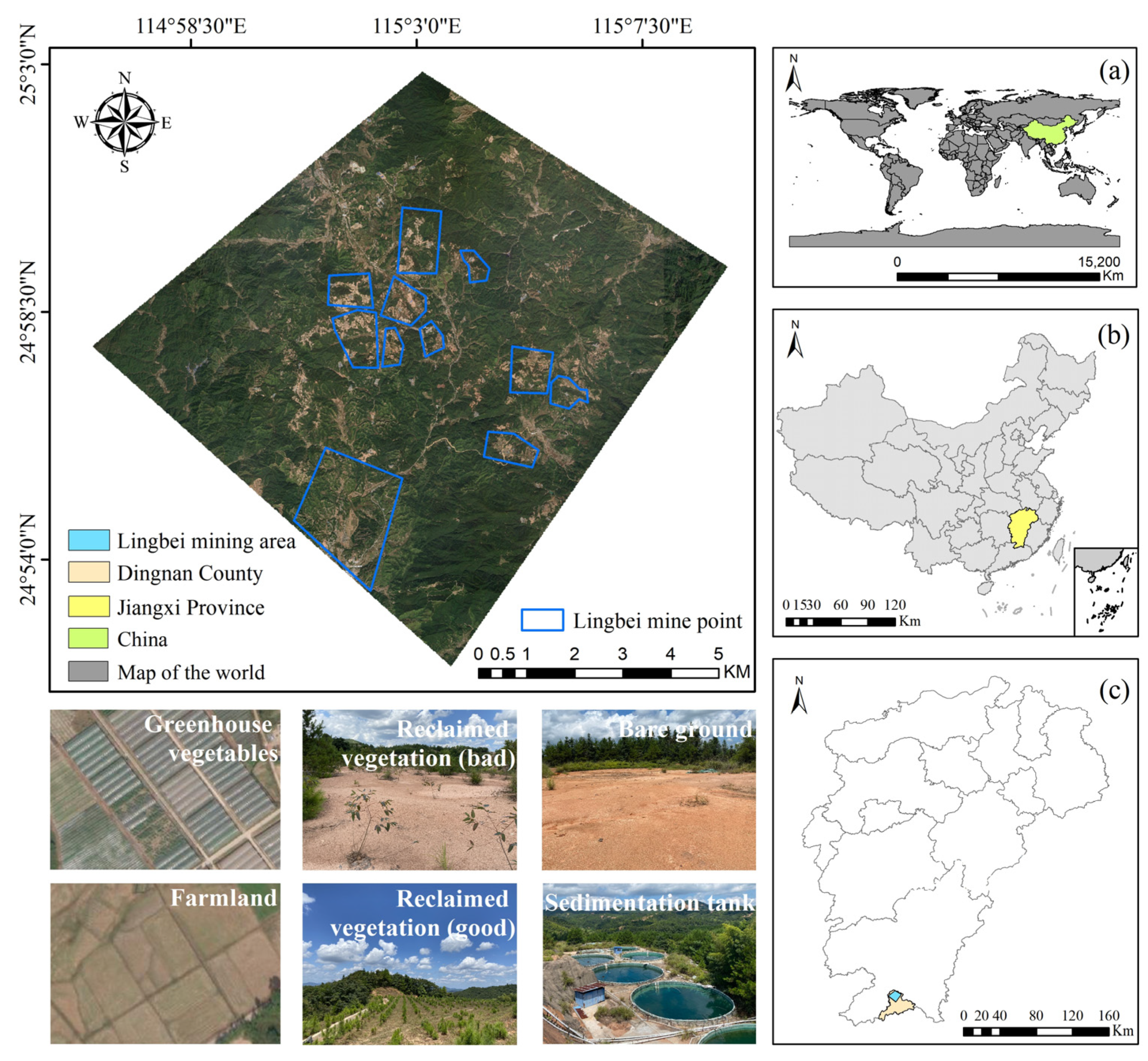
2.1. Overview of the Study Area

The Lingbei Rare Earth Mining Area is located at latitude 24°51′24″–25°02′56″ N and longitude 114°58′04″–115°10′56″ E; it is about 2 km north of Dingnan County, Jiangxi Province, China, has an area of about 213 km² (Figure 1), and has been mined for over 30 years. It has been affected by early unregulated mining processes and thus has undergone severe internal surface fragmentation, along with soil acidification and soil sanding due to prolonged mining. These phenomena occur intermittently, impeding the growth of vegetation and crops. The introduction of the Jiangxi Province Mineral Resources Master Plan (2008–2015) [18] has brought about some improvement in the ecological environment of the mining area. This improvement is evident in the alleviation of soil erosion and the restoration of the ecological environment, achieved through activities like cultivating various agricultural land classes such as orchards and reclaimed vegetation. Nevertheless, the presence of tailing land, bare land, sedimentation ponds, and other land classes arising from mining activities has complicated the surface of the mining area. This complexity poses challenges for effectively monitoring the development of agriculture and the ecological environment within the mining area.

2.2. Data Sources and Pre-Processing

The ‘Zhuhai-1 hyperspectral satellite’ (OHS) is a micro-nano satellite for remote sensing. It is financed, constructed, and operated by China’s Zhuhai Orbit Aerospace Science and Technology Company Limited. Currently, eight hyperspectral satellites orbit Earth. The OHS hyperspectral satellite carries a payload of Complementary metal-oxide-semiconductor (CMOS) detectors and is capable of acquiring data with a spatial resolution of 10 m and a spectral resolution of 2.5 nm [19], providing data covering 32 bands in the visible and near-infrared with a wavelength range of 400–1000 nm [19]. This information captures the visible- to near-infrared wavelength band, crucial for accurately identifying vegetation and other features.

This study used the OHS hyperspectral datasets consisting of clear and cloudless L1B level data acquired on 7 December 2021 from the OHS-2A satellite. These data include the RPC file, spatial extent file, and metadata file. Processing steps such as radiometric calibration, atmospheric correction, and orthometric correction need to be applied individually to the data. The study area is the Rare Earth Mining Area in Lingbei, China, with a spatial extent of 1916 × 1788 pixels.

2.3. Classification System and Sample Point Selection

The Bigmap GIS office sky map image (Bigmap v25.5.0.1) provides access to a variety of map information, including raster maps, satellite images, and aerial images. With a resolution of up to 0.5 m, it serves as valuable support for identifying detailed land classes [20]. Combining Bigmap and OHS hyperspectral images, the surface of the study area was divided into artificial surfaces and natural surfaces and then the artificial surfaces were divided into the human–work object class and the artificial building class to generate a classification system comprising 12 land classes (

Table 1. Land use classification scheme and image example of Lingbei rare earth mining area in Jiangxi Province.

	Land Class	Explicit Explanation	Examples of Bigmap GIS Office	Examples of OHS Hyperspectral Imagery
Artificial surface	Orchard (Ora)	The orchard is in the shape of a ladder with a distinct slope.
	Pool (Poo)	Ponds usually have edges that are easier to identify.
	Road (Roa)	Roads are generally long and continuous.
	Building (Bui)	Buildings are usually rectangular and neatly arranged.
	Farmland (Far)	It is composed of a large number of irregularly shaped plots closely connected, with obvious features.
	Sedimentation tank (Sed)	They are generally round and rectangular in shape and are densely distributed within a given area of the mine.
	Greenhouse vegetables (Gre)	It usually occurs in spring and winter and is more neatly arranged by adding tops to farm fields.
Natural surface	Unused land (Unu)	Mostly abandoned agricultural land, soils that are not planted with vegetation but show signs of cultivation, etc.
	Original vevetation (Ori)	Undeforested primary forests exist in large continuous areas.
	Reclaimed vegetation_good (Rec_g)	The saplings are regularly arranged, with good average growth, and are planted in an overall rectangular shape in the reclaimed area.
	Reclaimed vegetation_bad (Rec_b)	There is no clear pattern of saplings in the reclaimed area and their growth is clearly uneven, with the surrounding ground more similar to bare ground.
	Bare ground (Bar)	Land without any cover or treatment on the surface, generally located in the vicinity of mining areas.

Note: human-work object clas: Orc and Far; artificial building class: Roa, Bui, Poo, Gre, and Sed.

). The image was acquired in winter when farmers use greenhouses covered with plastic films to cultivate certain crops, extending the period of vegetable production. Therefore, the classification system encompasses both greenhouse vegetables and farmland. Given the noticeable differences in the growth of reclaimed vegetation in different areas, it is observed that some reclaimed vegetation is systematically arranged, predominantly rectangular in shape, with consistent and robust growth. In contrast, other areas of reclaimed vegetation lack regularity in distribution, showing uneven growth within the same reclaimed area. Additionally, these areas often exhibit bare ground near the vegetation. Therefore, the reclaimed vegetation is categorized into two groups: those with better growth and those with poorer growth.

The quality of the samples is directly related to the accuracy of the landform recognition in mining areas [9]. In this study, Bigmap is used for visual interpretation based on a classification system. Sample points are chosen, resulting in 2400 sample points of features—specifically 200 for each land class—after anomalous image element points are eliminated.

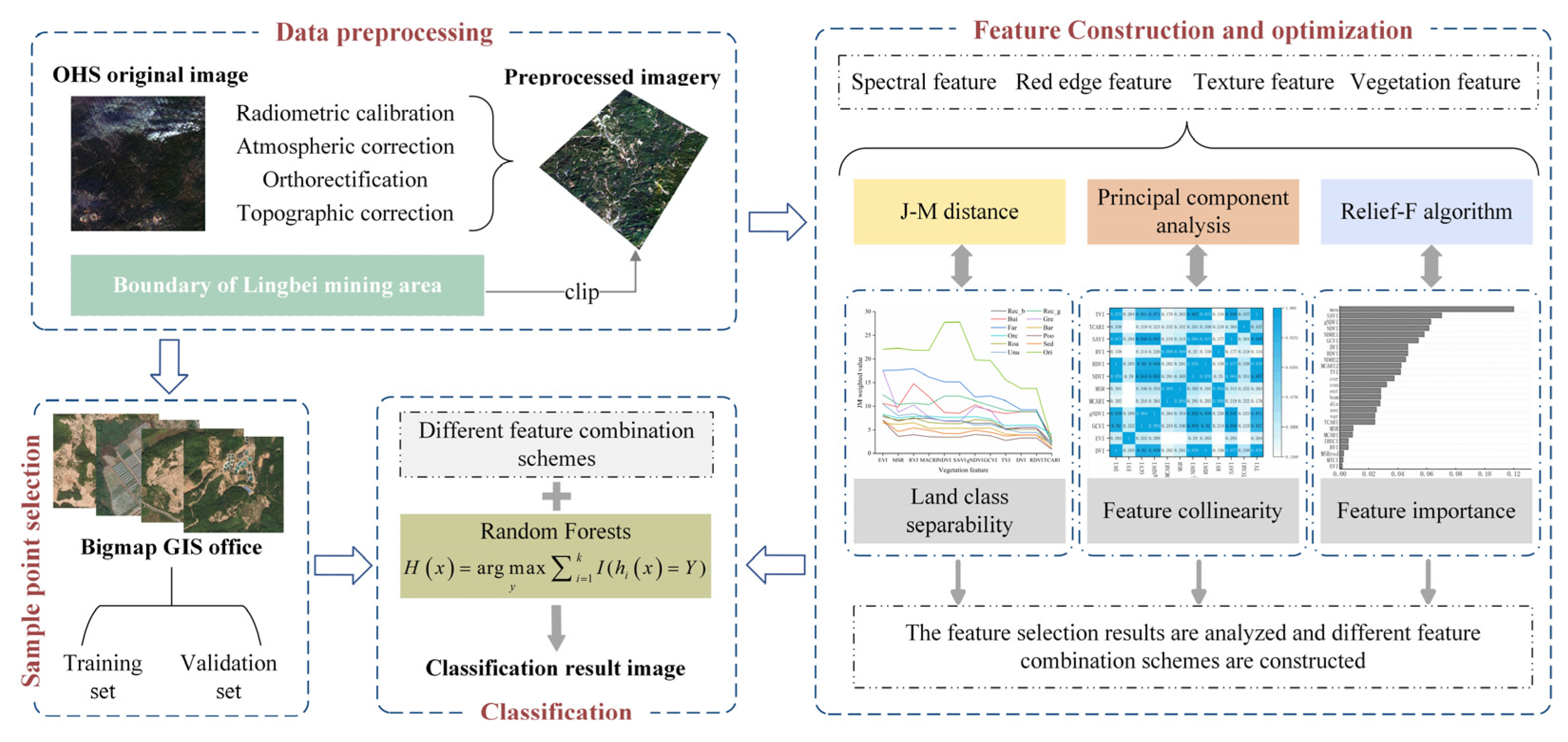
2.4. Research Method

Optimizing the constructed multiple feature categories and their associated feature indices involves analysis and screening of various features from different perspectives. This process is aimed at obtaining feature combinations that are more suitable for the fine classification of large-scale land use in mining areas, enhancing accuracy in classifying land use and precision in recognizing agricultural land classes. A technological flowchart is illustrated in Figure 2.

2.4.1. Feature Declaration

Due to the fragmentation of the surface and the complexity of the land classes in ion-adsorbing rare earth mining areas, the use of only traditional spectral features is not effective for the detailed classification of features and land class identification. Wanwan Yu et al. [21,22] showed that the addition of red-edge features can improve the separability between different land classes, which is promising for detailed land class identification and mapping. Therefore, 32 raw spectral reflectances from hyperspectral images were selected as input parameters to construct 12 vegetation indices and 6 red-edge indices. Pei Huan et al. [23] proposed that the participation of texture information from remote sensing images for classification can yield a better classification effect than only using spectral information and, therefore, in this study, eight kinds of texture indices based on the grayscale covariance matrix were constructed. In summary, four feature classes were selected in this study: spectral, vegetation, red edge, and texture features, as shown in

Table 2. Description of various characteristics.

Feature Variable	Index Abbreviation	OHS Image Calculation Formula	Exponential Description
Spectral feature	Band	B1, B2, …, B32
Vegetation feature	GCVI	$b27/b7-1$	Suitable for areas with high density vegetation cover.
	RDVI	$\left(b27-b13\right)/\sqrt{b27+b13}$	It can be used for high and low vegetation coverage.
	TCARI	$3\times \left[\left(b16-b14\right)-0.2\times \left(b16-b6\right)\times \left(\raisebox{1ex}{$b16$}\!\left/ \!\raisebox{-1ex}{$b14$}\right.\right)\right]$	It is very sensitive to changes in chlorophyll content.
	EVI	$2.5\times \left(\frac{b27-b13}{b27+6\times b13-7.5\times b1+1}\right)$	More sensitive to high vegetation coverage.
	NDVI	$\left(b27-b13\right)/\left(b27+b13\right)$	Characterize vegetation coverage and growth and health status.
	TVI	$0.5\times \left[120\times \left(b27-b7\right)-200\times \left(b13-b7\right)\right]$	Affected by chlorophyll and leaf tissue abundance, the difference between vegetation was obvious.
	SAVI	$\frac{b27-b13}{b27+b13+0.5}\times \left(1+0.5\right)$	It contains soil regulation coefficient and is more suitable for low vegetation cover area.
	MSR	$\left(\frac{b27}{b13}-1\right)/\sqrt{\frac{b27}{b13}}+1$	The index is based on an assessment of several vegetation indices derived from a combination of two spectral bands.
	RVI	$b27/b13$	It is used to estimate and measure vegetation biomass and is sensitive to high vegetation coverage.
	gNDVI	$\left(b27-b7\right)/\left(b27+b7\right)$	There was significant correlation with chlorophyll content and leaf area index.
	MACRI	$\left[\left(b27-b13\right)-0.2\times \left(b27-b7\right)\right]\times \left(b27/b13\right)$	It was responsive to chlorophyll concentration and background reflectance of leaves.
	DVI	$b27-b13$	It is sensitive to the change in soil background, and the sensitivity to vegetation decreases when the vegetation coverage is high.
Red edge feature	NDRE1	$\left(b19-b16\right)/\left(b19+b16\right)$	It can be used to estimate leaf area index and chlorophyll content of plants.
	NDRE2	$\left(b22-b17\right)/\left(b22+b17\right)$	It can be used in fine agriculture, vegetation stress detection, and so on.
	MSRred	$\left(b27/b16\right)-1/\sqrt{b27/b16}+1$	Replace the near infrared band in MSR with a valley with a red edge.
	MTCI	$b20-b17/b17-b15$	It is sensitive to chlorophyll content in plant leaves.
	MCARI_red	$1.5\times \frac{2.5\times \left(b23-b14\right)-1.3\times \left(b23-b6\right)}{\sqrt{{\left(2\times b23+1\right)}^2-\left(6\times b23-5\times \sqrt{b14}\right)-0.5}}$	It is more sensitive to the chlorophyll content in plants and the higher the value, the higher the chlorophyll content.
	IRECI	$\left(b22-b14\right)/\left(b16/b19\right)$	It is correlated with chlorophyll content and leaf area index of plant canopy and can quantitatively characterize chlorophyll content of plant.
Texture feature	Mean		Calculated based on the first four principal component bands after the original spectral principal component analysis, using window size: 5 × 5.
	Variance(Var)
	Homogeneity(Hom)
	Contrast(Con)
	Dissimilarity(Dis)
	Entropy(Ent)
	Second Moment(Sec)
	Correlation(Cor)

.

The results of the four feature categories above were combined sequentially to form seven different combinations of experimental schemes (

Table 3. Combination scheme information.

Combination Scheme	Specific Feature Information of the Scheme
Scheme 1	Spectral feature(Spe)(RF)
Scheme 2	Spectral feature+Vegetation feature(Spe+Veg)(RF)
Scheme 3	Spectral feature+Red edge feature(Spe+Red)(RF)
Scheme 4	Spectral feature+Texture feature(Spe+Tex)(RF)
Scheme 5	Spectral feature+Vegetation feature+Red edge feature+Texture feature(Spe+Veg+Red+Tex)(RF)
Scheme 6	Spectral feature+Feature importance ranking combination(Spe+Fea)(RF)
Scheme 7	Spectral feature+Vegetation feature+Red edge feature+Texture feature(Spe+Veg+Red+Tex)(SVM)

). These schemes were designed to investigate how the accuracy of land use classification in rare earth mining areas changes when incorporating vegetation features, red-edge features, and texture features using the RF classification algorithm. From them, we can determine the single feature category with the most significant effect on improving the accuracy of land-use fine classification on a large scale in mining areas and identify agricultural land classes, including farmland. In addition, these schemes allow us to intuitively explore whether the proposed feature selection method effectively enhances the accuracy of land-use fine classification and agricultural land identification. The objective was to compare the schemes to identify the optimal feature combinations suitable for the detailed classification of large-scale land use and the identification of agricultural land classes in rare earth mining areas.

2.4.2. Feature Optimization Methods

Although the expansion and combination of feature variables can provide better classification results, using all the features for the classification may lead to information redundancy, resulting in a “curse of dimensionality”, which could impact the classification performance [24]. Therefore, using the same feature class as a benchmark and performing feature optimization on it can yield feature variables that are more favorable for fine-grained feature classification in mining areas with various types of features. In order to select feature indices with a higher separability of features and at the same time avoid covariance among indices, we utilized the J-M (Jeffreis-Matusita) distance and principal component analysis for feature variable optimization in the different feature categories.

The J-M distance provides superior results among the many methods for separability determination [25,26]. It can determine the variability between categories based on the degree of separation, with values ranging from 0 to 2—the larger the value, the better the separation. For the training sample set E (i, j = 1, 2,…, N, i ≠ j) in two to-be-separated land classes w_i and w_j, assuming that m_i and m_j are the feature means of w_i and w_j and τ_i and τ_j are the feature standard deviations of w_i and w_j, the mathematical expression of the J-M distance is as follows:

$$J=2\left(1-e^{-B}\right)$$

(1)

$$B=\frac{1}{8}{\left(m_i-m_j\right)}^2\frac{2}{{\tau }_i^2+{\tau }_j^2}+\frac{1}{2}\ln \frac{{\tau }_i^2+{\tau }_j^2}{2{\tau }_i{\tau }_j}$$

(2)

where J denotes the J-M distance and B denotes the Bachmann distance.

To address variations in differentiation among land classes, we further process the J-M distance by introducing weighting. These weights are determined based on the criterion that the more indistinguishable the combination of land classes, the larger the weights, and vice versa. In this study, we initially categorize land use in mining areas into two major groups: highly distinguishable artificial and natural land surfaces (Table 1). These two major categories are then assigned weight values equal to 1. In addition, the artificial land surface category is divided into two subcategories: artificial objects and artificial construction. These subcategories are assigned a weight value of 2, particularly for clearly distinguishable land classes such as farmland and buildings. Finally, weights between land classes within the same type of land use are assigned values of 3 or 4, determined by the degree of similarity between features. The weights for specific landform combinations are presented in

Table 4. Weight allocation of land class combination.

Land Assemblage	Weights	Land Assemblage	Weights	Land Assemblage	Weights
Rec_b, Far	2	Rec_g, Far	3	Gre, Roa	2
Rec_b, Rec_g	4	Far, Bar	2	Gre, Sed	2
Rec_b, Bar	4	Far, Ora	3	Bar, Ora	2
Rec_b, Ora	2	Far, Unu	4	Bar, Roa	4
Rec_b, Unu	3	Far, Ori	2	Bar, Unu	3
Rec_b, Ori	2	Rec_g, Bar	2	Ora, Unu	2
Bui, Gre	4	Rec_g, Ora	3	Ora, Ori	2
Bui, Roa	2	Rec_g, Unu	2	Poo, Sed	3
Bui, Sed	2	Rec_g, Ori	4	Roa, Sed	2
Unu, Ori	2

; those not listed carry a weight of 1. We used the weighted J-M distance to analyze vegetation, red edge, and texture features. Feature variables exhibiting a strong differentiation of landforms are identified as the preferred characteristics.

Principal component analysis (PCA) is a powerful technique for dimensionality reduction and feature selection. With PCA, a low-dimensional feature space composed of projection directions can better reflect the spatial structure information of the original high-dimensional data [27,28] and facilitate the interdependence and correlation analysis of features [29]. As many as 32 original spectral bands are provided by OHS hyperspectral datasets. Moreover, using PCA for dimensionality reduction effectively addresses the “dimensionality catastrophe” problem while substantially preserving the original band information. Covariance between feature variables can lead to the inclusion of features that do not enhance classification accuracy because of the diverse features used in this study. Thus, in the current study, correlation tests for vegetation, red edge, and texture features were separately conducted using principal component analysis. Feature variables with minimal covariance were prioritized for the classification of land use to mitigate the adverse effects of covariance.

2.4.3. Importance Ranking of Features

The ranking of features by importance can help to filter out features with high contributions to classification, regression, and other problems from multiple features in a short time, improve calculation speed, and reduce the dimensions of data input [30]. This study ranked the importance of all feature indices, encompassing vegetation, red edge, and texture characteristics. This ranking provides an overall assessment of the contribution of each feature type to classification. It allows for an intuitive identification of feature categories and indices suitable for detailed feature classification in mining areas. The Relief-F algorithm, a classic multivariate filtering feature selection method used in various classification problems, assigns weights to features based on their relevance to the landform class. Features weighing less than a specified threshold are rejected [31]. The algorithm is computed as follows: given class labels, there are l classes C = [C₁, C₂,…, C_l], a sample R_i is randomly selected from the training set, then k approximate samples of R_i are identified in the same class, denoted as H_j (j = 1,2,…, k), and k approximate samples of R_i are also identified from different categories, denoted as M_j(C) (j = 1,2,…, k), which repeats the above steps on each feature dimension and obtains each feature weight as follows:

$$W(A)=W(A)-{\displaystyle \sum _{j=1}^k\frac{diff(A,R_i,H_j)}{m\ast k}}+{\displaystyle \sum _{C\ne class(R_i)}[\frac{P(C)}{1-P(class(R_i))}\times {\displaystyle \sum _{j=1}^k\frac{diff(A,R_i,M_j(C))}{m\ast k}}}$$

(3)

where A denotes the feature, W(A) denotes the weight of feature A, m is the number of iterations, and P(C) denotes the probability that the category is C. diff(A, R_i, H_j) and diff(A, R_i,M_j(C)) denote the difference between the samples R_i and H_j, M_j(C), respectively, with respect to A, which is defined as follows:

$$diff(A,R_1,R_2)=\left\{\begin{array}{c}\frac{R_1\left[A\right]-R_2\left[A\right]}{\mathit{max}\left(A\right)-\mathit{min}\left(A\right)},\hspace{0.33em}if\hspace{0.33em}A\hspace{0.33em}is\hspace{0.33em}continuous\\ 0,\hspace{0.33em}if\hspace{0.33em}(A\hspace{0.33em}is\hspace{0.33em}discrete)\hspace{0.33em}and\hspace{0.33em}(R_1\left[A\right]\hspace{0.33em}=\hspace{0.33em}{R}_2\left[A\right])\\ 1,\hspace{0.33em}if\hspace{0.33em}(A\hspace{0.33em}is\hspace{0.33em}discrete)\hspace{0.33em}and\hspace{0.33em}(R_1\left[A\right]\hspace{0.33em}\ne \hspace{0.33em}{R}_2\left[A\right])\end{array}\right.$$

(4)

where R₂ stands for H_j, M_j(C).

2.4.4. Land Use Classification

The RF algorithm facilitates the integration of high-dimensional data from multiple sources, rendering it suitable for complex datasets [32]. It exhibits high adaptability to overfitting in training samples and accomplishes classification tasks within a brief duration. The results of a study on the classification of Mediterranean shrub vegetation types in the Languedoc region of southern France showed that the RF algorithm outperforms traditional classifiers in the identification of hyperspectral vegetation types for automatic classification and is especially advantageous for distinguishing vegetation types with small spectral differences [33]. The input classification data of the study included spectral features, vegetation features, red edge features, and texture features, which involve more complex data with higher dimensions. The study area constitutes various land classes with smaller spectral differences. Therefore, the RF algorithm is effective and offers certain advantages for the detailed classification of land use in mining areas. RF adopts Bootstrap resampling to build a decision tree model for each of the k samples selected from the training sample set. After each tree is classified, the final classification result is determined by voting [34].

$$H\left(x\right)=\underset{y}{\arg \max }{\displaystyle {\sum }_{i=1}^{k}I(h_i\left(x\right)=Y)}$$

(5)

where H(x) denotes the combination of classification models, h_i denotes the decision tree classification model, Y denotes the output variable, and I(°) is the indicator function.

2.4.5. Accuracy Verification

In order to compare the effects of incorporating different features on the accuracy of feature classification, this study evaluates the overall accuracy by using the confusion matrix. The confusion matrix can help evaluate the accuracy by comparing the degree of confusion between the classification results and the actual measurements and includes the overall accuracy (OA), Kappa coefficient, producer’s accuracy (PA), and user’s accuracy (UA). Among them, the overall accuracy and Kappa coefficient are used to evaluate the overall performance of the classifier and the producer’s accuracy and user’s accuracy are used to evaluate the misclassification and omission indicators of a particular class.

$$OA=\frac{{\displaystyle {\sum }_{i=1}^K{N}_{ii}}}{N}$$

(6)

$$Kappa=\frac{N{\displaystyle {\sum }_{i=1}^K{N}_{ii}-{\displaystyle {\sum }_{i=1}^K{N}_{i+}{N}_{+i}}}}{N^2-{\displaystyle {\sum }_{i=1}^K{N}_{i+}{N}_{+i}}}$$

(7)

$$P{A}_i=\frac{N_{ii}}{N_{+i}}$$

(8)

$$U{A}_i=\frac{N_{ii}}{N_{i+}}$$

(9)

where N represents the total number of samples; K represents the total number of categories; N_ii represents the number of samples assigned to the correct category; and N_+i and N_i+ represent the true number of samples in category i and the number of samples predicted to be in category i, respectively.

3. Results

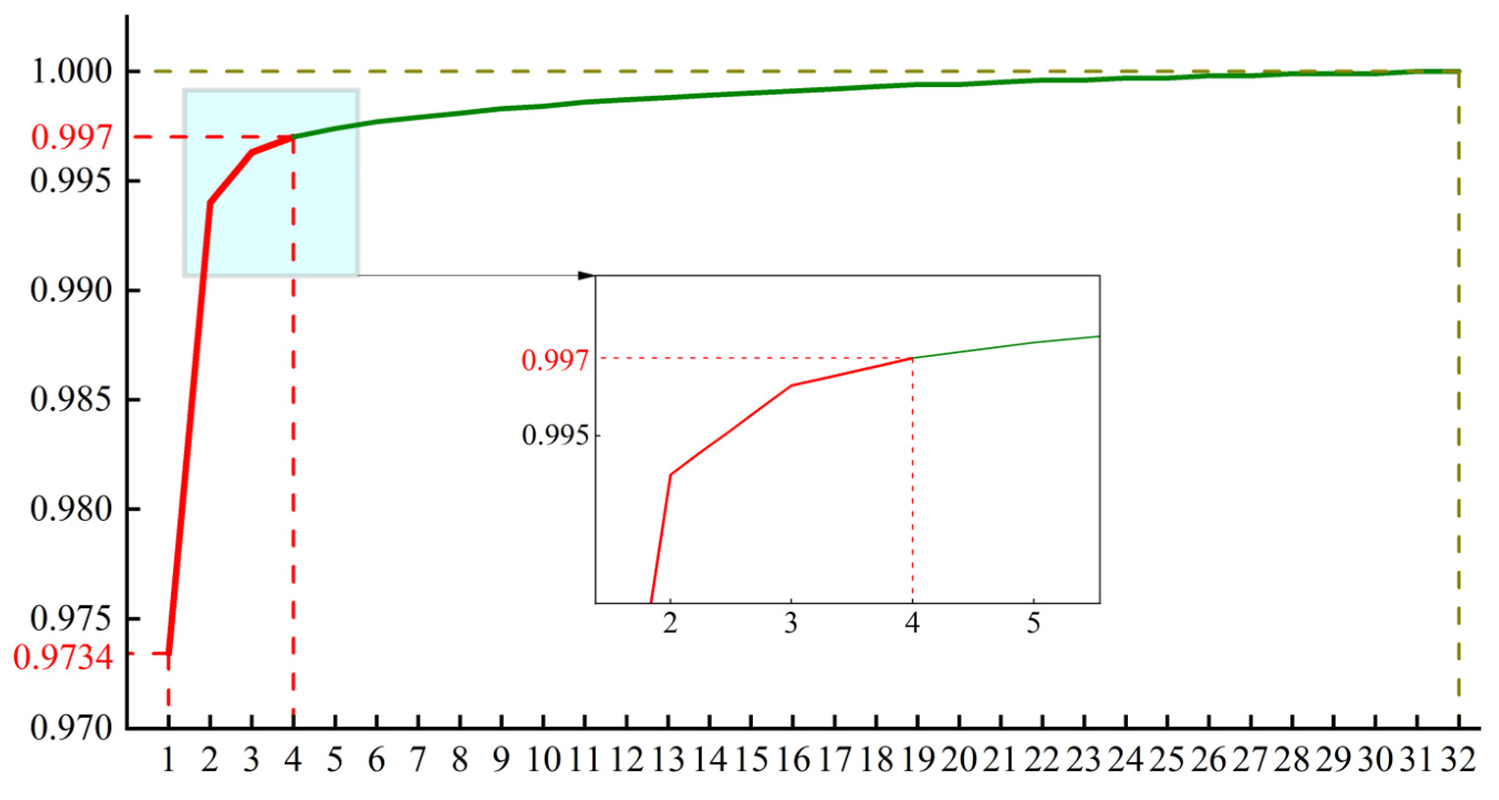
3.1. Feature Optimization Results

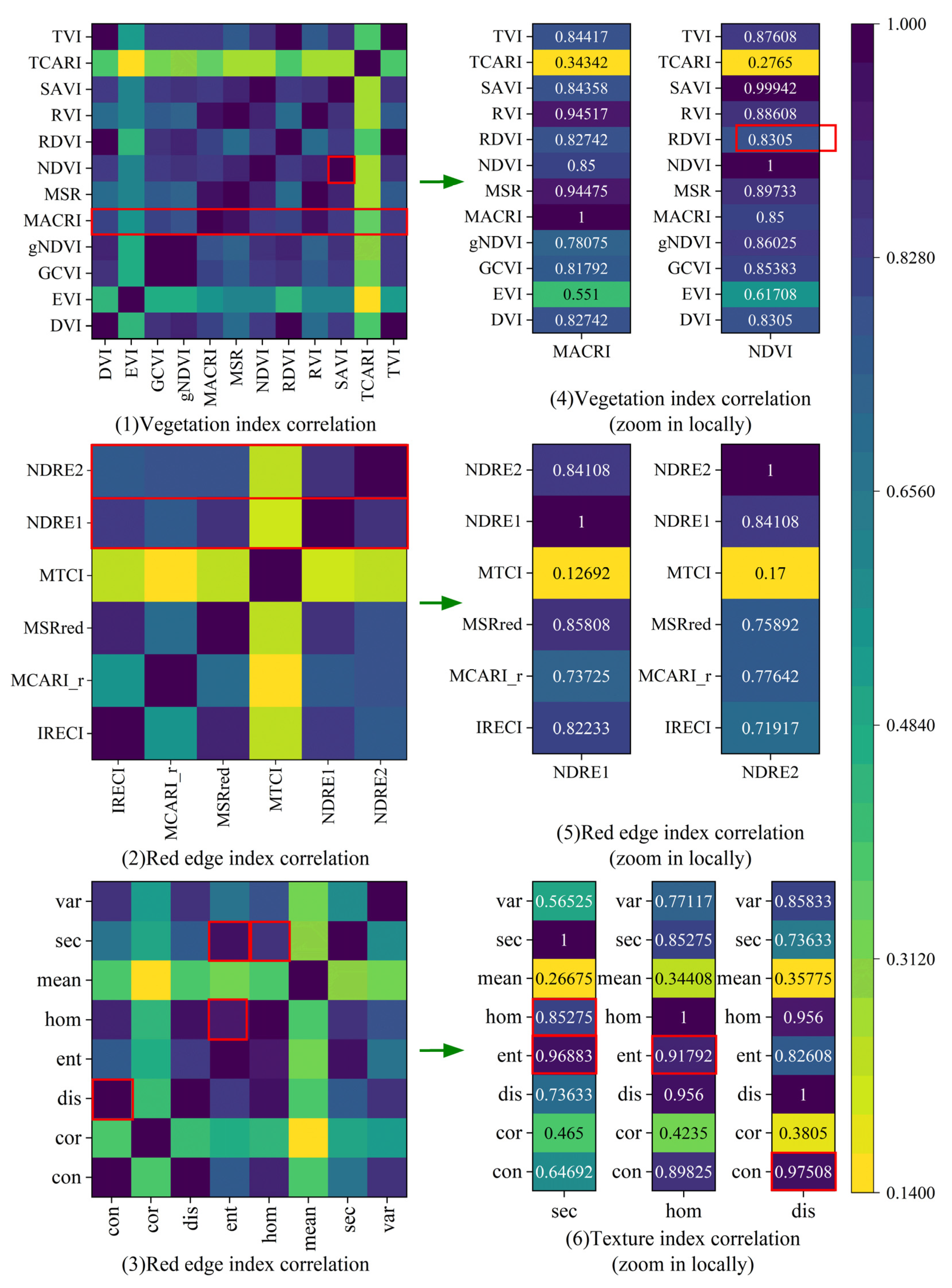
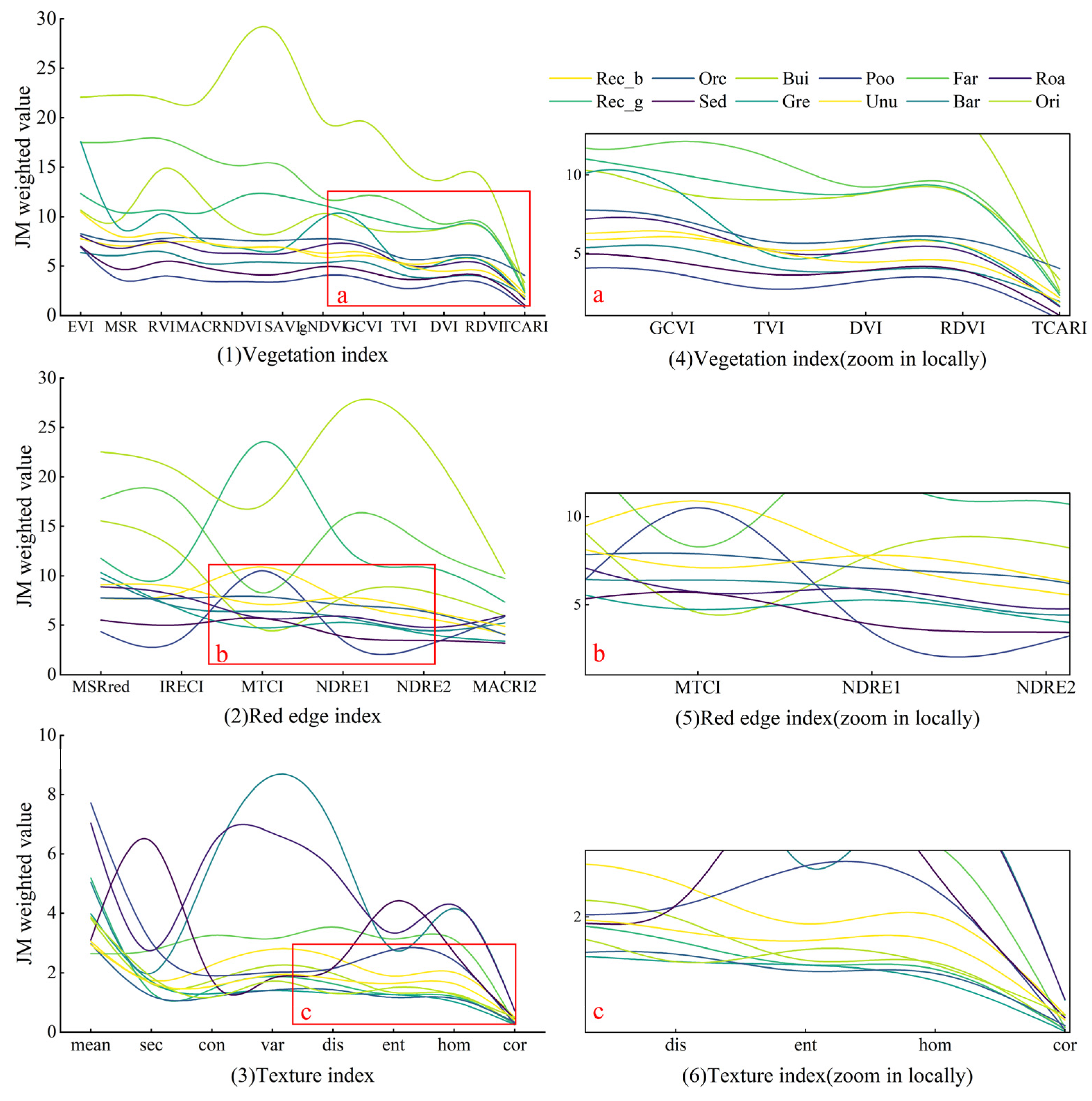
3.1.1. Determination of Spectral Features

Spectral features were calculated and downscaled using principal component analysis. The contribution of each principal component was used as a benchmark to rank them cumulatively, as shown in Figure 3, where the horizontal coordinates indicate the new spectral bands generated by the principal component analysis of the original spectral features and the vertical coordinates indicate the cumulative contribution of the new spectral bands to the image information. Among them, the cumulative contribution rate of the first principal component to the fourth principal component increases more in relative order and, from the fourth principal component onwards, the growth rate of the contribution rate decreases and the contribution rate value stabilizes above 0.997. Therefore, this study finally selects the first four principal components as the result of the final spectral feature preference.

3.1.2. Determination of Vegetation Features

The 12 vegetation indices were subjected to weighted J-M distance calculations and principal component analysis and the results are shown in Figure 4 and Figure 5. Figure 4 shows that most of the vegetation indices have good divisibility of features and some of them have outstanding divisibility of specific features but that the divisibility ability of TVI, DVI, RDVI, and TCARI for the land classes is not ideal, which is in line with the fact that although they are sensitive to the content of chlorophyll and so on, most of the land classes are construction land, mining land, etc. [35]. Figure 5 shows that the correlation coefficient between NDVI and SAVI is close to 1, which is a strong correlation between the two, and therefore, NDVI was preferred considering that it has a better ability to characterize the surface reflectance of the features than SAVI [36]. MCARI was not considered because it had a strong correlation with most of the indices. Therefore, the vegetation characteristics were finally filtered to GCVI, EVI, NDVI, MSR, RVI, and gNDVI.

3.1.3. Determination of Red Edge Features

The red edge features were also feature optimized using weighted J-M distance and principal component analysis, as shown in Figure 4 and Figure 5. The figures show that both NDRE1 and NDRE2 have low separability for most of the land classes and that the degree of correlation with the other indices is high. Therefore, the final selected red-edge features are MSRred, MTCI, MCARI_Red, and IRECI.

3.1.4. Determination of Texture Features

The method of feature preference for texture features is the same as that for vegetation features and red edge features, as shown in Figure 4 and Figure 5. Figure 4 shows that the separability of cor for each class is obviously extremely low and the separability of hom for each class, although higher than cor, is still downstream compared to the other indices. Figure 5 shows that sec, ent, and hom have a high correlation, con and dis have a high correlation, and con and sec are more divisible when compared to each other and, therefore, the preferred texture features were finally determined to be mean, var, con, and sec.

Figure 4. JM distance weights and detail curves of each feature on different ground classes. (“a” shows the index curve with significantly worse JM weighted value in the vegetation index; “b” is the exponential curve with significantly worse JM weighting value in the red edge index; “c” shows the exponential curve with significantly poor JM weighting in the texture index.).

Figure 4. JM distance weights and detail curves of each feature on different ground classes. (“a” shows the index curve with significantly worse JM weighted value in the vegetation index; “b” is the exponential curve with significantly worse JM weighting value in the red edge index; “c” shows the exponential curve with significantly poor JM weighting in the texture index.).

Figure 5. The correlation between the features of heat maps and high values of specific parts.

Figure 5. The correlation between the features of heat maps and high values of specific parts.

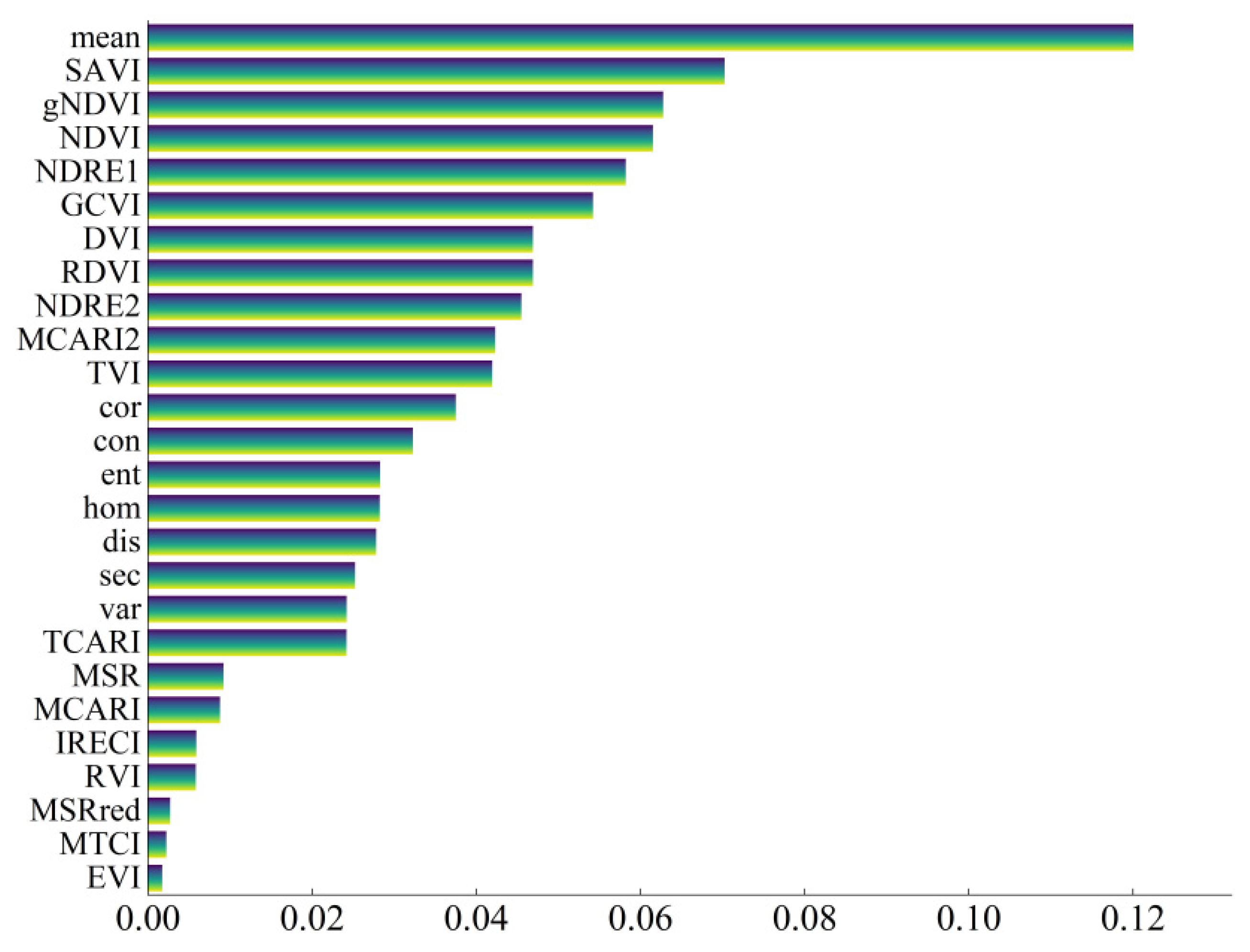
3.2. Importance Ranking of Characteristic Variables

The Relief-F algorithm was used to evaluate and sort the importance of all the feature variables. The results are shown in Figure 6: texture index mean had the highest score and was much higher than the other indexes, reaching 0.1200. The vegetation index SAVI, gNDVI, and NDVI decreased successively. NDRE1, the red index, secured the fifth position. The vegetation index in the upper and middle reaches of the score was higher and the other texture indexes except the mean were mostly in the middle reaches of the score. The index of the downstream region is the red edge index and vegetation index and half of the red edge index is in this region. After comprehensive consideration, the importance of feature variables was ranked in descending order as follows: texture feature, vegetation feature, and red edge feature.

Among the three types of feature variables selected, the feature importance of the red-edge feature ranked last, which is related to the actual land class categories in the study area: the most different spectral characteristics of green vegetation and other features is the significant increase in reflectance in the red-edge band [37]. However, the image-capturing time was December, when some crops were processed into greenhouse vegetables to ensure their continued growth and the land classes in the complex parcels in mining areas mostly consisted of buildings, bare ground, sedimentation tanks, and other construction land. The vegetation land class in the overall land class accounted for a relatively small portion and, therefore, the red edge features failed to add constructively to the distinction between land classes. Additionally, the mining area encompasses various features such as farmland, greenhouse vegetables, sedimentation tanks, and bare ground, where texture information is more pronounced. Particularly, the texture features not only demonstrate a certain advantage in the detailed identification of plastic greenhouses [38] but also improve the classification and identification accuracy of texture information-rich land classes [24], providing a distinct advantage in the identification of land classes within mining areas. This is consistent with the texture index “MEAN” being ranked first and being significantly higher than the other indexes.

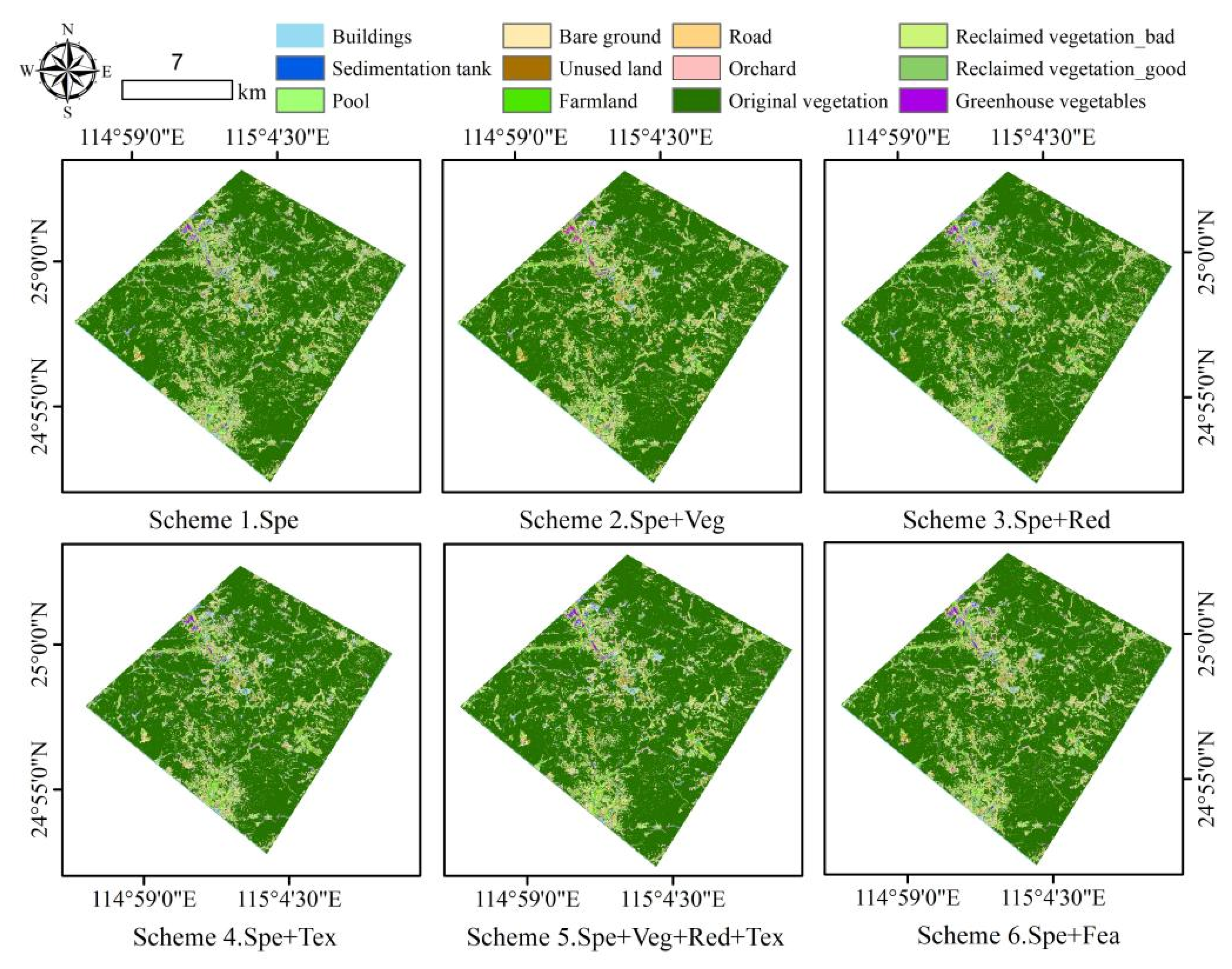
3.3. Accuracy Evaluation of Land Use Classification in Mining Area

This study adopts overall accuracy, Kappa coefficient, producer’s accuracy, and user’s accuracy as the evaluation indexes of the land use classification results of mining areas and compares the classification results of the seven schemes; the classification accuracy and classification results of the schemes are shown in

Table 5. Precision statistics of the classification results of each scheme.

Classifications		Scheme 1	Scheme 2	Scheme 3	Scheme 4	Scheme 5	Scheme 6	Scheme 7
Overall Accuracy		83.59%	85.56%	84.52%	86.68%	88.43%	88.26%	88.16%
Kappa coefficient		0.51	0.55	0.53	0.58	0.62	0.59	0.61
Buildings	PA%	82.06	81.29	83.59	82.36	85.74	80.21	84.97
	UA%	57.47	63.70	52.40	63.25	58.84	66.88	56.07
Sedimentation tank	PA%	25.48	26.44	25.00	35.58	38.94	17.79	31.73
	UA%	12.83	15.71	15.25	16.37	24.92	14.23	21.36
Pool	PA%	82.82	86.50	68.71	74.85	61.96	68.71	67.48
	UA%	13.53	15.06	13.49	17.40	21.40	14.18	22.40
Bare ground	PA%	41.29	41.94	40.65	56.13	50.97	34.19	49.68
	UA%	4.26	4.93	3.96	7.95	7.47	12.77	7.59
Farmland	PA%	52.04	51.68	58.54	65.51	66.98	54.52	64.86
	UA%	83.27	83.33	87.24	89.22	91.01	78.96	91.12
Road	PA%	100.00	100.00	100.00	100.00	100.00	91.67	100.00
	UA%	3.46	3.54	4.08	3.66	3.58	1.96	3.79
Orchard	PA%	28.38	25.73	27.32	25.20	28.91	4.24	28.65
	UA%	12.74	13.31	19.54	11.63	17.17	3.02	15.91
Original vevetation	PA%	89.33	91.41	89.93	91.82	93.71	95.20	93.57
	UA%	99.24	99.17	99.24	99.21	99.22	99.29	99.19
Reclaimed vegetation_good	PA%	37.19	32.46	38.99	37.03	36.22	15.50	36.54
	UA%	19.81	24.81	17.92	28.13	29.40	20.79	28.75
Reclaimed vegetation_bad	PA%	27.45	27.12	33.99	29.41	32.03	24.35	30.72
	UA%	24.21	25.74	33.66	30.20	36.57	22.11	36.22
Greenhouse vegetables	PA%	50.90	61.44	52.33	60.68	61.16	60.11	60.78
	UA%	70.81	73.69	70.73	66.91	74.62	72.01	70.25
Unused land	PA%	50.00	55.71	55.71	67.14	62.86	85.71	67.14
	UA%	12.46	10.66	13.88	16.97	14.47	12.55	15.31

Note: PA: producer accuracy; UA: user accuracy.

, Figure 7 and Figure 8, and the confusion matrix of the scheme with the best classification results is shown in Figure 9. The overall classification accuracy is the lowest when only using the spectral features after principal component analysis of the original spectrum for the extraction of rare earth mining area classes; the overall accuracy and Kappa coefficient are only 83.59% and 0.51, respectively. Schemes 2, 3, and 4, respectively, include the vegetation features, red edge features, and texture features after feature optimization on the basis of the spectral features and the classification accuracy increases compared with that of Scheme 1, which is specifically represented by the overall accuracy increase of 1.97%, 0.93%, and 3.09% respectively, indicating that the inclusion of vegetation features, red edge features, and texture features can effectively improve the classification accuracy of land use in rare earth mining areas; here, the texture features have the greatest effect on the improvement in accuracy. Scheme 5 integrates the spectral features and feature indices after feature selection from each feature category and the overall accuracy and Kappa coefficient are again improved significantly. The overall accuracy of Scheme 5 is the highest among all schemes, being improved by 4.84%, and the Kappa coefficient is improved by 0.11. Scheme 7 uses SVM to classify the same combination of features and its accuracy is slightly lower than that of Scheme 5, which indicates that RF works better than other classifiers such as SVM for the detailed classification of large-scale land use in mining areas; after adopting the importance ranking of feature variables for the classification of surface cover in mining areas (Scheme 6), the total feature preference results in overall accuracy and Kappa coefficient values that are essentially equivalent to those of Scheme 5. The user accuracies of farmland and greenhouse vegetables are greatly improved in Scheme 4, which correlates with the strong texture information of these two types of agricultural features. The user accuracies of orchards and reclaimed vegetation are better in Scheme 3, indicating that the red-edge features are able to differentiate and recognize these two types of agricultural land classes from the complex surface environment. A comprehensive analysis of the user accuracy of the above four agricultural land classes in different programs shows that both Program 5 and Program 6, which are based on the RF algorithm, are able to recognize them relatively effectively; the user accuracy of Program 5 is higher than that of Program 6 in general.

Overall, the feature preference method used by the Institute not only effectively improves the accuracy of the detailed classification of land use in mining areas but also accurately extracts agricultural land classes such as farmland, orchards, reclaimed vegetation, and greenhouse vegetables from complex land classes, thus supporting the understanding and monitoring of agricultural development within mining areas.

4. Discussion

Hyperspectral datasets have multiple narrow bands and contain a large amount of information, enabling more accurate and detailed feature variables to be obtained. Based on the OHS hyperspectral datasets, four kinds of feature datasets were constructed: spectral, vegetation, red edge, and texture features. J-M distance calculation and principal component analysis were carried out for the indices of the different feature categories. This process aimed to uncover the separability of feature indices to land classes and assess the covariance between feature indices within the same land classes. This approach was employed to achieve a more rational and detailed feature preference. The Relief-F algorithm was used to rank the importance of features, excluding spectral features, and a more precise and detailed feature preference was obtained from the overall features. This approach provided feature preference results from an overall perspective, enabling an analysis to identify the most effective feature categories for the detailed classification of land use in mining areas. Based on the above analysis method, seven different combinations of feature variables were designed and the effects of different indices on classification accuracy in different schemes were analyzed using an RF algorithm to explore the feature preference combinations applicable to land use classification in mining areas and for agricultural land class identification. The study results indicate that after feature optimization, all features of each category attain varying degrees of improvement in classification accuracy (Table 5). (1) Texture features exert the most pronounced effect on overall accuracy across all categories, consistent with their high significance in feature importance analysis. Notably, incorporating texture features leads to significant enhancements in classification accuracy for farmland, greenhouse vegetables, and other texture-rich land classes. Conversely, red-edge features exert the least influence on overall; however, they more effectively recognize agricultural land classes, such as farmland and reclaimed vegetation within complex land parcels, compared with other indices. This observation aligns with the recognized issue of severe fragmentation in farmland and reclaimed vegetation arising from uncontrolled mining in mining areas. Integrating red-edge features effectively reduces landscape fragmentation and improves recognition accuracy [39]. Both types of indices contribute to the accurate identification of agricultural land classes, facilitating precise monitoring of agricultural development. (2) Among all schemes, combining the index results of each category features yields the highest classification accuracy. It can also comprehensively meet the requirements for improving the identification accuracy of different types of agricultural land. These findings suggest that the feature selection method used in the current study can provide more appropriate feature optimization results. The approach not only enables fine-scale land use classification in mining areas on a large scale but also ensures accurate recognition of different agricultural land classes within mining areas. This method provides technical support for monitoring agricultural development in mining areas and offers effective recommendations for further agricultural and ecological sustainability.

In summary, (1) hyperspectral datasets hold promise for the detailed land use classification of large-scale complex landforms and (2) the feature selection method is effective in reducing feature dimensions and improving classification accuracy. Hyperspectral images can contain hundreds of subdivided spectral bands at consecutive wavelengths, yielding rich spectral information and enabling more detailed detection and identification of target features [40]. Many studies have been conducted to utilize hyperspectral datasets for classification, such as Zhao Peng et al. [41] who fused texture features and spectral features and combined these with hyperspectral images to identify timber species; their classification accuracy was higher than that of traditional methods. Fei Xing et al. [8] used a hybrid analysis method of multiple end-element spectral analysis and extracted alpine grassland cover using hyperspectral images. Binge Cui et al. [10] classified small scenes of coastal wetlands using hyperspectral images and achieved robust results. Although previous studies using hyperspectral datasets have achieved better extraction or classification results, the research objects were mostly single species or small scenes. There is limited research on the detailed classification of large-scale complex surface areas. To address this gap, this study employs in-orbit hyperspectral images for detailed land use classification in mining areas. Notably, it demonstrates the robustness of the classification accuracy remains, regardless of the inclusion of features beyond spectral features. In order to further verify the advantages of hyperspectral imagery for complex surface classification, we compare the results of this study with those conducted for other similar mining areas. Zhang Chengye et al. [42] used HF2 imagery to classify the surface of mining areas, dividing it into eight categories, of which the overall accuracy was only 80.10% even though the classification accuracy of the restoration and management areas, open-pit quarries, and water bodies were as high as 95.00%, 85.10%, and 72.5%, respectively. Although the spatial resolution of the OHS hyperspectral datasets used in this study is only 10 m, which is not better than that of the Gaofen-2 image with a spatial resolution of better than 1 m, the spectral resolution is as high as 2.5 nn and, therefore, it contains more detailed spectral information of the landforms. Furthermore, the degree of spectral differentiation of the complex landforms is stronger, so the classification precision is obviously higher and the overall classification precision obtained using spectral indices alone is already 83.59%. The overall accuracy of classification using only the spectral index is 83.59%. The use of hyperspectral datasets for land use classification on a large scale in mining areas can improve accuracy, facilitating the extraction of necessary information from complex surfaces to meet research requirements.

Due to the large number of bands contained in hyperspectral images and the various feature variables that can be obtained from them, it is highly likely that the direct use of all these features for classification will result in dimensional redundancy, which will have an impact on classification accuracy [43]. To address this situation, many researchers have used different feature preference methods for dimensionality reduction, such as Mahdianpari et al. [44] who used the J-M distance to quantitatively analyze the separability of different types of wetlands under different features; they then classified the land classes after feature selection based on the separability results, which resulted in robust classification accuracy. Md Rashedul et al. [45] combined MMF and mRMR methods for the dimensionality reduction in feature variables. Hao Yufeng et al. [46] and Fushuyu et al. [47] performed variable optimization for wetland classification through the Relief-F algorithm and RFE algorithm, respectively. Xiang Songyang et al. [30] selected features involved in hyperspectral image classification by constructing the ReliefF-RFE feature selection algorithm. Although all of the above studies used feature selection methods to derive effective preferred features, most of them only considered land class separability or feature relevance individually. In this study, we comprehensively considered the separability of land classes and the covariance between features, not only analyzing each class of features individually for feature selection but also mining the feature indices of different feature classes that are applicable to the detailed classification of mining areas. We then ranked the importance of feature class indices other than the spectral features to analyze the most important feature classes in terms of the detailed classification of a wide range of mining areas. By designing a multi-program format and using RF algorithms to explore the effects of the optimal combination of feature indices after the above multi-faceted analysis, we effectively explored the optimal feature classes and feature combination programs for detailed and large-scale land use classification in mining areas and the identification of agricultural land classes such as farmland. The study results indicate that the proposed feature preference method enhances both the fine classification of land use and the identification of agricultural land classes. This technique aids in monitoring agricultural development in mining areas and advancing sustainable agriculture and ecological practices.

5. Conclusions

The primary aim of this research is to leverage hyperspectral imagery in constructing diverse feature sets and employ a range of feature selection methods to pinpoint the most suitable combination of features for rare earth mining areas. This endeavor seeks to facilitate the refined classification of land use within expansive and intricate mining territories, enabling the accurate identification of agricultural land types like farmland, orchards, and reclaimed vegetation from fragmented data. Such efforts are instrumental in advancing agricultural development monitoring, guiding sustainable agricultural practices, and fostering ecological sustainability. The results show that

(1) The feature preference method combining J-M distance and principal component analysis provides a better feature combination scheme from the perspective of land class separability and feature correlation. It improves the accuracy of land use classification in mining areas and agricultural land class identification significantly;

(2) Ranking the importance of the other three categories of features, excluding spectral features, shows that the degree of importance of features in the land use classification of rare earth mining areas is as follows: texture index, vegetation index, and red edge index;

(3) Combining the indices of the four features after feature optimization yielded the most significant improvement in land use classification accuracy for mining areas, reaching 88.43%, with a Kappa coefficient of 0.61. This performance not only surpasses the overall classification accuracy achieved using a single feature but also simultaneously results in an effective increase in classification accuracy for specific farmland classes such as farmland, orchards, reclaimed vegetation, and greenhouse vegetables.

Using hyperspectral datasets and feature selection methods, this study has led to enhanced accuracy in fine land surface coverage classification in mining areas and the identification of agricultural land classes. It lends technical support for monitoring agricultural conditions in mining areas and promoting sustainable development. However, the extent to which these results can be applied to other mining areas remains uncertain. This uncertainty arises from the limitations imposed by the study area’s environment, the classification of land classes, the time period, and other factors. Therefore, in the future, more study areas can be added to further explore the universality of the research methods and results.

References

1. Shi, X.Y.; Chen, H.W. Study on the pollution path and remediation of ionized rare earth ores in waste pond leaching reactor. Chin. J. Rare Earth Sci. 2019, 37, 409–417. (In Chinese) [Google Scholar]
2. Zou, G.L.; Wu, Y.D.; Cai, S.J. Effect of ionic rare earth leaching process on resources and Environment. Nonferrous Met. Sci. Eng. 2014, 5, 100–106. (In Chinese) [Google Scholar]
3. Li, Y.; Li, H.; Xu, F. Spatiotemporal changes in desertified land in rare earth mining areas under different disturbance conditions. Environ. Sci. Pollut. Res. 2021, 28, 30323–30334. [Google Scholar] [CrossRef]
4. Zhang, Y.H.; Zhao, X. Land-Use and Land-Cover Change Detection Using Dynamic Time Warping–Based Time Series Clustering Method. Can. J. Remote Sens. 2020, 46, 67–83. [Google Scholar] [CrossRef]
5. Xiao, Y.; Jiang, Q.G.; Wang, B.; Li, Y.H.; Liu, S.; Cui, C. Object-oriented land use classification based on mixed feature selection of Relief F and PSO. Trans. Chin. Soc. Agric. Eng. 2016, 32, 211–216. (In Chinese) [Google Scholar]
6. Zhang, Z.M.; Liu, B.; Guan, X. Land Use Type Change in the Upper Yellow River Basin Coal Mining Area and Its Impact on Carbon Sequestration Services. Environ. Sci. Res. 2024, 37. (In Chinese) [Google Scholar] [CrossRef]
7. Xu, J.X.; Chen, C.; Zhou, S.T.; Hu, W.M.; Zhang, W. Land use classification in mine-agriculture compound area based on multi-feature random forest: A case study of Peixian. Front. Sustain. Food Syst. 2024, 7, 1335292. [Google Scholar] [CrossRef]
8. Zheng, Y.; Wang, Y.; Liu, Y. Vegetation classification and recognition of mountain meadow based on seasonal characteristics of hyperspectral data. Spectrosc. Spectr. Anal. 2022, 42, 1939–1947. (In Chinese) [Google Scholar]
9. Tu, C.R.; Li, P.; Li, Z.H.; Wang, H.J.; Yin, S.W.; Li, D.H.; Zhu, Q.T.; Chang, M.X.; Liu, J.; Wang, G.Y. Synergetic Classification of Coastal Wetlands over the Yellow River Delta with GF-3 Full-Polarization SAR and Zhuhai-1 OHS Hyperspectral Remote Sensing. Remote Sens. 2021, 13, 4444. [Google Scholar] [CrossRef]
10. Xing, F.; An, R.; Guo, X.L.; Shen, X.J.; Soubry, I.; Wang, B.L.; Mu, Y.M.; Huang, X.L. Mapping Alpine Grassland Fraction Coverage Using Zhuhai-1 OHS Imagery in the Three River Headwaters Region, China. Remote Sens. 2023, 15, 2289. [Google Scholar] [CrossRef]
11. Qin, P.; Cai, Y.L.; Wang, X.L. Small Waterbody Extraction With Improved U-Net Using Zhuhai-1 Hyperspectral Remote Sensing Images. IEEE Geosci. Remote Sens. Lett. 2022, 19, 1–5. [Google Scholar] [CrossRef]
12. Zhou, G.L.; Ni, Z.Y.; Zhao, Y.B.; Luan, J.W. Identification of Bamboo Species Based on Extreme Gradient Boosting (XGBoost) Using Zhuhai-1 Orbita Hyperspectral Remote Sensing Imagery. Sensors 2022, 22, 5434. [Google Scholar] [CrossRef]
13. Cui, B.G.; Li, X.H.; Wu, J.; Ren, G.B.; Lu, Y. Tiny-Scene Embedding Network for Coastal Wetland Mapping Using Zhuhai-1 Hyperspectral Images. IEEE Geosci. Remote Sens. Lett. 2022, 19, 1–5. [Google Scholar] [CrossRef]
14. Mo, Y.; Zhong, R.F.; Cao, S.S. Orbita hyperspectral satellite image for land cover classification using random forest classifier. J. Appl. Remote Sens. 2021, 15, 014519. [Google Scholar] [CrossRef]
15. Wang, Z.H.; Zhao, Z.; Yin, C.L. Fine Crop Classification Based on UAV Hyperspectral Images and Random Forest. ISPRS Int. J. Geo-Inf. 2022, 11, 252. [Google Scholar] [CrossRef]
16. Somnath, P.; Nikhil, R.D.; Mukunda, D.B.; Bimal, K.B.; Jadunandan, D. Species-level classification of mangrove forest using AVIRIS-NG hyperspectral imagery. Remote Sens. Lett. 2023, 14, 522–533. [Google Scholar]
17. Qin, H.M.; Zhou, W.Q.; Yao, Y.; Yao, W.M. Individual tree segmentation and tree species classification in subtropical broadleaf forests using UAV-based LiDAR, hyperspectral, and ultrahigh-resolution RGB data. Remote Sens. Environ. 2022, 280, 113143. [Google Scholar] [CrossRef]
18. Liu, J.F.; Hu, X. Overall Planning of Mineral Resources in Jiangxi Province 2008–2015; Jiangxi Science and Technology Press: Nanchang, China, 2011. [Google Scholar]
19. Zhuhai Orbita Aerospace Micro Technology Co., Ltd. Available online: https://www.myorbita.net/index.aspx (accessed on 21 February 2024).
20. BIGMAP. Available online: http://www.bigemap.com/ (accessed on 21 February 2024).
21. Yu, W.W.; Zhao, P.; Xu, K.J.; Zhao, Y.J.; Shen, P.J.; Ma, J.J. Evaluation of red-edge features for identifying subtropical tree species based on Sentinel-2 and Gaofen-6 time series. Int. J. Remote Sens. 2022, 43, 3003–3027. [Google Scholar] [CrossRef]
22. Guo, Y.C.; Ren, H.R. Remote sensing monitoring of maize and paddy rice planting area using GF-6 WFV red edge features. Comput. Electron. Agric. 2023, 207, 107714. [Google Scholar] [CrossRef]
23. Pei, H.; Sun, T.J.; Wang, X.Y. Object-oriented land use/cover classification based on Landsat 8 OLI image texture. Trans. Chin. Soc. Agric. Eng. 2018, 34, 248–255. (In Chinese) [Google Scholar]
24. Wang, L.J.; Kong, Y.R.; Yang, X.D.; Xu, Y.; Liang, L.; Wang, S.G. Land use classification of agricultural areas based on feature optimization random forest algorithm. Trans. Chin. Soc. Agric. Eng. 2020, 36, 244–250. (In Chinese) [Google Scholar]
25. Wang, C.X.; Ma, N.; Ming, Y.F.; Wang, Q.; Xia, J.F. Classification of hyperspectral imagery with a 3D convolutional neural network and J-M distance. Adv. Space Res. 2019, 64, 886–899. [Google Scholar] [CrossRef]
26. Sun, Z.P.; Shen, W.M.; Wei, B.; Liu, X.M.; Su, W.; Zhang, C.; Yang, J.Y. Object-oriented land cover classification using HJ-1 remote sensing imagery. Sci. China Ser. D Earth Sci. 2010, 53, 34–44. [Google Scholar] [CrossRef]
27. Zhang, X.; Chen, B.Z.; Zhao, H.; Fan, H.D.; Zhu, D. Soil Moisture Retrieval over a Semiarid Area by Means of PCA Dimensionality Reduction. Can. J. Remote Sens. 2016, 42, 136–144. [Google Scholar] [CrossRef]
28. Wang, X.F.; Lu, C.H.; Li, J.X.; Liu, J. Generalized cosine two-dimensional principal component analysis. Acta Autom. Sin. 2022, 48, 2836–2851. (In Chinese) [Google Scholar]
29. Jason, Y.; Du, X.R. An enhanced water index in extracting water bodies from Landsat TM imagery. Ann. GIS 2017, 23, 141–148. [Google Scholar]
30. Xiang, S.Y.; Xu, Z.H.; Zhang, Y.W.; Zhang, Q.; Zhou, X.; Yu, H.; Li, B.; Li, Y.F. Construction and application of ReliEF-RFE feature Selection Algorithm for hyperspectral image classification. Spectrosc. Spectr. Anal. 2022, 42, 3283–3290. (In Chinese) [Google Scholar]
31. Yu, X. A feature selection approach based on NSGA-II with ReliefF. Appl. Soft Comput. 2023, 134, 109987. [Google Scholar]
32. Li, H.K.; Wang, L.J.; Xiao, S.S. Land use random forest classification in southern hilly region based on multi-source data. Trans. Chin. Soc. Agric. Eng. 2021, 37, 244–251. (In Chinese) [Google Scholar]
33. Sabat-Tomala, A.; Raczko, E.; Zagajewski, B. Comparison of support vector machine and random forest algorithms for invasive and expansive species classification using airborne hyperspectral data. Remote Sens. 2020, 12, 516. [Google Scholar] [CrossRef]
34. Xi, Y.; Ren, C.; Wang, Z.; Wei, S.; Bai, J.; Zhang, B.; Xiang, H.; Chen, L. Mapping tree species composition using OHS-1 hyperspectral data and deep learning algorithms in Changbai mountains, Northeast China. Forests 2019, 10, 818. [Google Scholar] [CrossRef]
35. Meng, Q.Y.; Dong, H.; Qin, Q.M.; Wang, J.L.; Zhao, J.H. A plant cover index MTCARI for monitoring vegetation chlorophyll content based on hyperspectral remote sensing. Spectrosc. Spectr. Anal. 2012, 8, 2218–2222. (In Chinese) [Google Scholar]
36. Kodimalar, T.; Vidhya, R.; Eswar, R. Land surface emissivity retrieval from multiple vegetation indices: A comparative study over India. Remote Sens. Lett. 2020, 11, 176–185. [Google Scholar] [CrossRef]
37. Tian, X.Y.; Zang, Y.H.; Liu, R.; Wei, J.J. Study on multi-temporal Sentinel-2 large-scale winter wheat extraction considering vegetation red edge information. J. Remote Sens. 2022, 26, 1988–2000. (In Chinese) [Google Scholar]
38. Wu, J.Y.; Liu, X.L.; Bo, Y.C.; Shi, Z.T.; Fu, Z. Identification of plastic greenhouses based on GF-2 data combined with multi-texture features. Trans. Chin. Soc. Agric. Eng. 2019, 35, 173–183. (In Chinese) [Google Scholar]
39. Liu, J.; Wang, L.; Teng, F.; Yang, L.; Gao, J.; Yao, B.; Yang, F. Impact of red-edge waveband of RapidEye satellite on estimation accuracy of crop planting area. Nongye Gongcheng Xuebao/Trans. Chin. Soc. Agric. Eng. 2016, 32, 140–148. [Google Scholar]
40. Hong, D.F.; Wu, X.; Ghamisi, P.; Chanussot, J.; Yokoya, N.; Zhu, X.X. Invariant Attribute Profiles: A Spatial-Frequency Joint Feature Extractor for Hyperspectral Image Classification. IEEE Trans. Geosci. Remote Sens. 2020, 58, 3791–3808. [Google Scholar] [CrossRef]
41. Zhao, P.; Han, J.C.; Wang, C.K. Classification of wood species by hyperspectral microscopic imaging based on I-BGLAM texture and spectral fusion. Spectrosc. Spectr. Anal. 2021, 41, 599–605. (In Chinese) [Google Scholar]
42. Zhang, C.Y.; Li, F.Y.; Li, J.; Xing, J.J.; Yang, J.Z.; Guo, J.T.; Du, S.H. Land use classification of open pit coal mine based on DeepLabv3+ and GF-2 high-resolution images. Coal Geol. Explor. 2022, 50, 94–103. (In Chinese) [Google Scholar]
43. Rashedul, I.; Boshir, A.; Ali, H. Feature reduction of hyperspectral image for classification. J. Spat. Sci. 2022, 67, 331–335. [Google Scholar]
44. Masoud, M.; Bahram, S.; Fariba, M. The First Wetland Inventory Map of Newfoundland at a Spatial Resolution of 10 m Using Sentinel-1 and Sentinel-2 Data on the Google Earth Engine Cloud Computing Platform. Remote Sens. 2019, 11, 43. [Google Scholar]
45. Islam, M.R.; Siddiqa, A.; Ibn, A.M.; Uddin, M.P.; Ulhaq, A. Hyperspectral Image Classification via Information Theoretic Dimension Reduction. Remote Sens. 2023, 15, 1147. [Google Scholar] [CrossRef]
46. Hao, Y.F.; Man, W.D.; Wang, J.H.; Liu, M.Y.; Zhang, K. Wetland information extraction based on Relief-F algorithm and decision tree method. J. Liaoning Tech. Univ. (Nat. Sci. Ed.) 2021, 40, 225–233. (In Chinese) [Google Scholar]
47. Xie, S.Y.; Fu, B.L.; Li, Y.; Liu, Z.L.; Zuo, P.P.; Lan, F.W.; He, H.C.; Fan, D.L. Research on classification method of swamp wetland in Honghe National Nature Reserve based on multi-dimensional remote sensing image. Wetl. Sci. 2021, 19, 1–16. (In Chinese) [Google Scholar]
Figure 1. Geographical location and surface condition of the Lingbei mining area. ((a) Location information of China on the world map; (b) Location information of Jiangxi Province in China; (c) Location information of the study area in Jiangxi Province.).
Sustainability 16 03582 g001
Figure 2. Technology roadmap.
Sustainability 16 03582 g002
Figure 3. Cumulative contribution rate of principal components.
Sustainability 16 03582 g003
Figure 6. Rank of the importance of different features (the bar indicates the magnitude of the importance score for each feature index).
Sustainability 16 03582 g006
Figure 7. Results of land use classification under different schemes.
Sustainability 16 03582 g007
Figure 8. Comparison of feature-specific classifications of land use classifications under Scheme 5.
Sustainability 16 03582 g008
Figure 9. Scheme 5 confusion matrix for land use classification. (The red numbers represent the number of pixels correctly classified for each land use classification in Scheme 5. Commission and Omission represent the misclassification and missed classification errors for each land-use category in Scheme 5, respectively, with lighter colors indicating smaller errors.).
Sustainability 16 03582 g009