Oil Depletion and the Energy Efficiency of Oil Production: The Case of California

Abstract
: This study explores the impact of oil depletion on the energetic efficiency of oil extraction and refining in California. These changes are measured using energy return ratios (such as the energy return on investment, or EROI). I construct a time-varying first-order process model of energy inputs and outputs of oil extraction. The model includes factors such as oil quality, reservoir depth, enhanced recovery techniques, and water cut. This model is populated with historical data for 306 California oil fields over a 50 year period. The model focuses on the effects of resource quality decline, while technical efficiencies are modeled simply. Results indicate that the energy intensity of oil extraction in California increased significantly from 1955 to 2005. This resulted in a decline in the life-cycle EROI from ≈6.5 to ≈3.5 (measured as megajoules (MJ) delivered to final consumers per MJ primary energy invested in energy extraction, transport, and refining). Most of this decline in energy returns is due to increasing need for steam-based thermal enhanced oil recovery, with secondary effects due to conventional resource depletion (e.g., increased water cut).1. Introduction: Oil Depletion and the Energy Return of Low Quality Oil Resources
A transition in oil production has been occurring for decades: the fuels that consumers put into their automobiles are being produced using increasingly energy-intensive production methods, and from resources other than “conventional” oil. This transition is the result of three trends occurring worldwide: output from existing oil fields is declining, new fields are not as large or productive as old fields, and areas with conventional resources are increasingly off-limits to investment by independent oil companies. These trends are inducing investment in substitutes for conventional petroleum, such as the Alberta tar sands, or synthetic fuels from coal or oil shale [1].
Historically, the most common substitutes for conventional oil have been low-quality hydrocarbons, such as the heavy oils in California and bitumen in Alberta. These resources are more difficult to extract than conventional petroleum, are more difficult to refine into finished fuels, and are more expensive. Much of this increased cost and difficulty is due to larger energy demands for extraction and refining. For example, in California, thermally-produced heavy oil requires the injection of steam to decrease the oil viscosity and induce flow within the reservoir. Also, refining heavy oil is more energy intensive due to the fact that it is hydrogen deficient and often impurity-laden.
This oil transition will cause growing tension in the coming decades: a transition to low-quality oil resources will reduce our ability to improve the environmental profile of energy production—an imperative for the twenty-first century—but increasing demand for fuel from developing countries could increase market instability and competition over constrained oil resources.
The nature of oil depletion is understood mostly by studying aggregate statistics such as regional production curves [2–4]. Due to the lack of publicly available data, little research has been performed on the specific effects of depletion on oil operations (e.g., effects of depletion on required capital investment versus operating expenses). Also, only a small amount of attention in the peer-reviewed literature has been paid to the energy efficiency impacts of oil depletion [5,6].
This paper seeks to explore these energy efficiency impacts by building a detailed model of California oil production over time. First this paper presents a history of California oil production, focusing on changing oil resource quality and resource depletion. Next, methods for calculating energy inputs and outputs from oil production are described. Using these energy inputs and outputs, energy return ratios are computed using methods of life cycle assessment (LCA) and net energy analysis (NEA). Lastly, results from these calculations are presented and their broader significance is discussed.
2. An Industrial History of California Oil Production: Resource Quality, Depletion, and Innovation
2.1. Early Oil Production Before 1900
Pre-commercial use of oil in California included use by Native Americans for coating, sealing and adhesion [7]. Early commercial production was concentrated in the San Joaquin valley of California, where low-quality surface oil was mined in pits and tunnels [8]. The first refinery—a simple still for batch processing with a capacity of 300 gallons—was constructed near McKittrick in 1866, but it soon failed due to poor economics and high transport costs [7]. Figure 1 shows historical milestones in the California oil industry plotted along with production volumes [9,10].
By the 1890s, surface mining had declined in importance and the cable tool rig had become the standard drilling method in California. Power for the cable tool rig was provided by a steam engine, and drilling power increased rapidly: Drake's famous rig generated 4.4 kilowatts (kW) in 1859, and by 1900, steam boilers were rated at 29 kW, and the attached steam engines were rated at 18 kW [7].
Oil became a socially and economically dominant industry in the San Joaquin Valley with the discovery of the Kern River field in May of 1899. The proximity of this field to Bakersfield allowed the shipment of oil via rail to San Francisco. By 1903, Kern River production increased to 17 million barrels per year, or ≈ 70% of California's production. No gushers were ever found in the Kern River field, due to its low initial pressure (1.2–3.8 megapascal (Mpa) and heavy viscous oil (0.96–1.0 specific gravity, and up to 10,000 centipoise viscosity) [11].
Early oil production was inefficient and wasteful, due to a combination of poor knowledge of geological principles and poor ability to control production. Early producing wells often declined rapidly, particularly in the Los Angeles basin [7]. This is because producers would withdraw and often vent or flare the associated gas, depleting the reservoir drive. These depleted wells, generally producing only a few barrels per day, were often sold off by their operators. Industrious producers would buy up contiguous depleted wells and apply technology to increase production. Operators would commonly attach a central oil-fired pumping unit to serve numerous wells simultaneously [7]. This represents an early example of self-consumption of oil by producers to offset the effects of depletion.
2.2. Early 20th Century Production: 1900–1940
The first recorded attempt at thermal enhanced oil recovery (EOR) was by J.W. Goff in 1901 [7]. He had no experience in the oil industry, but he attempted to solve the problems of the producers in the Kern River field, who struggled with its heavy oil. He injected steam, air, and steam-heated air into wells. Goff achieved a small amount of incremental production, but depressed oil prices stymied his early attempt at EOR [7].
An important technological development in the early 1900s was the advent of the rotary drilling rig as a replacement for the cable-tool rig. The first committed effort to rotary drilling in California was by Standard Oil in 1908. Early rotary rigs were powered by steam engines, which were replaced by internal combustion engines by the 1930s. Rotary drilling eventually dominated oil well drilling, as it was faster and more effective.
Efforts in the late 1920s and 1930s focused most visibly on attempting to drill deeper. Deep oil had been found at Kettleman hills: 635 m3/d (4000 bbl/d) from a single well, 2133 m deep, producing valuable light oil (0.74 specific gravity) [12]. This encouraged others to drill deeper wells in existing fields. Thermal methods were also experimented with briefly in this period, with the Tidewater oil company injecting hot water into the Casmalia field in 1923 (Casmalia oil is dense and viscous, having a specific gravity as high as 1.015 [11]).
These early attempts at enhanced oil recovery were not successful, as ample production from high-quality light oil fields at the time made these operations costly and unneeded. Per-well yearly production rates peaked in the 1930s, reaching ≈ 24,000 bbl/well in 1930 and declining thereafter to less than 5,000 bbl/well in the current day.
2.3. The Modern Era of California Oil Production: 1940 to 2000
In the post-war period, discovery of large new fields declined. Research attention focused on ways to extract a larger share of California's vast heavy oil resources. Knowing that heat reduces the viscosity of crude oil, in 1956 engineers attempted to light a fire downhole in the Midway-Sunset field by injecting air and using a novel electric ignition system. This method is called in situ combustion or “fireflooding”. The ignition system was unnecessary, as injected air caused spontaneous combustion [13].
Other companies utilized bottomhole heaters. These heaters took heat generated at the surface and transmitted it to the formation using a heat exchanger. These had much lower capital costs than the air compression equipment required for fireflooding (1 M$ for compressor vs. 3000$ for a bottomhole heater) [13]. The biggest success for the bottomhole heaters occurred in the Kern River field. Engineers concluded that heat conduction from the bottomhole heaters was slow and ineffective, and that more effective thermal production would require injecting heat-conducting fluid into the reservoir body.
The first modern steam injection project recorded in California was in April of 1960. Shell had studied potential steam injection processes in the laboratory and carried out secret pilot projects at the Yorba Linda field (specific gravity of 0.986) [13]. This was followed by a Kern River project in August of 1962 [14]. The success of these projects caused rapid spread of the technology across the industry. Many steam injection projects were built quickly: in 1964 and 1965 more than 50 steam injection projects were initiated each year [14]. Production increased significantly in fields where steam injection was instituted (see Table 1).
Oil production continued to increase in the 1960s. Production increased to over 160 × 103 m3/d (1 Mbbl/d) in the mid 1960s, reaching a plateau that lasted ≈ 20 years [15]. Simultaneously, production per well dropped, reaching 4 m3/well-d (25 bbl/well-d) in 1963 and never rising above this level again [15]. This is because much of the incremental production in this period was not from new large fields or gushers, but instead from increasing the intensity of extraction in depleted fields using advanced recovery technologies. Infill drilling (the drilling of wells on closer spacing in already producing fields) was aided by powerful drilling rigs: by the 1980s, rigs put out ≈ 350–850 kW, or 11–30 times the output of rigs from the turn of the century [16].
In the late 1970s and 1980s, regulatory attention focused on air quality impacts of thermal enhanced oil recovery. The California Air Resources Board (CARB) studied the problem between 1979 and 1983 [16]. Because unrefined crude oil was burned for steam generation, emissions from steam generators contained sulfur, nickel, and vanadium. By 1982 a variety of regulatory controls were in place [17], and over the course of the 1980s, EOR boilers were largely converted to natural gas fuel.
Concerns about energy efficiency of steam injection caused cogeneration of heat and power to be implemented in California TEOR projects in the 1980s. In 1978, the California Energy Commission (CEC) considered the feasibility of cogeneration in California thermally enhanced oil operations [18]. Projects were added throughout the 1980s and 1990s, and generation capacity from these oilfield projects reached ≈ 2000 MW by 2004, or 4% of California's electricity generation capacity [19]. Air quality regulations have reshaped thermal oil recovery: only three projects remain that use petroleum coke and coal, and no projects use oil produced from the field itself, the primary fuel for all early oil field steam generation projects. Both major steam injection projects in the Los Angles air basin were closed in 1999, due in part to the cost of emissions allowances [19].
Total California oil production reached its peak in 1984 at ≈ 190×l03 m3/d (1.2 Mbbl/d), and is in terminal decline (see Figure 1) [20]. Per-well yearly production rates are currently less than 5,000 bbl/well, down from a peak of ≈ 24,000 bbl/well in 1930. Over 17% of California oil production in 2008 was produced from stripper wells—defined by the California Department of Oil, Gas, and Geothermal Resources as wells producing less than 10 barrels per well per day. Some 59% of operating wells in California are now classified as stripper wells [21].
3. Methods—Energy Return Ratios Based on a Bottom-up Life Cycle Framework
This study quantifies the energy efficiency impacts of oil depletion in California using methods of life cycle assessment (LCA) [22,23] and net energy analysis (NEA) [24,25]. The analysis requires calculating energy inputs and outputs from all process stages, in a similar fashion to LCA. This set of flows will allows “bottom-up” calculation of net energy returns at either the point of extraction or at the point of consumption of finished fuel (full-fuel cycle EROI). This bottom-up approach differs from “top-down” approaches based on aggregate industry statistics or reported economic flows between sectors.
To quantify these effects, a time series of life cycle energy inputs and outputs from oil extraction is constructed. Dynamic or time-varying LCA has been performed in the past using a variety of methods. Pehnt studied the impacts of renewable energy technologies over time, finding that the impacts become less over time as the result of increasing efficiency of materials extraction and refining [26]. Levasseur et al. have constructed a framework for dynamic accounting of GHG impacts given time variation in releases and the decay characteristics of GHGs over time [27]. Most closely related to this effort, Mendivil et al. studied the changes over time in the life cycle air emissions from ammonia synthesis from 1950 to 2000 [28]. Using information from patents and industry literature, they constructed an LCA model of different types of ammonia technology, and estimated emissions resulting from each technology over time.
3.1. A Bottom-Up Model of Energy Inputs and Outputs
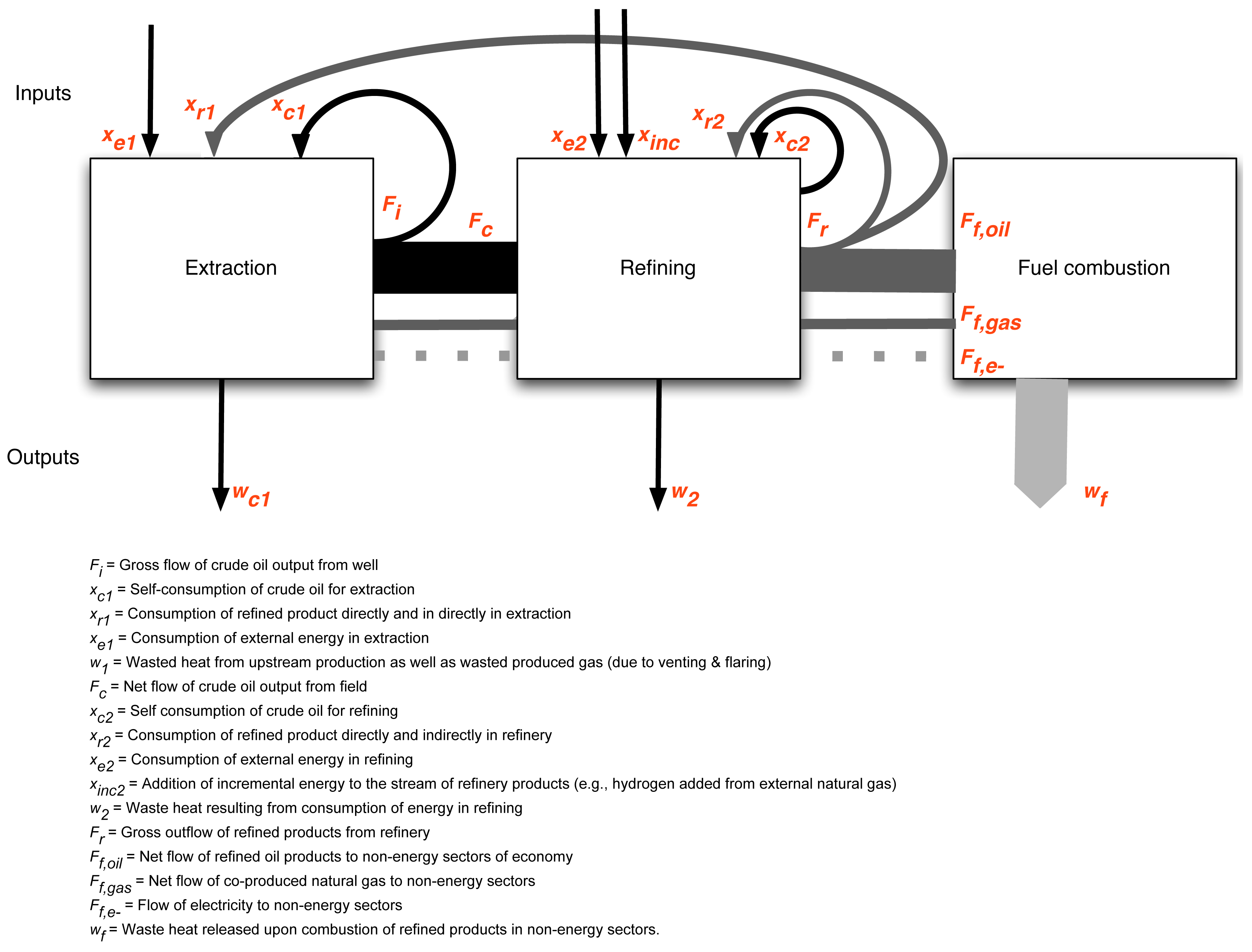
Our process model (see Figure 2) includes three process stages: primary energy extraction, upgrading of primary energy into forms usable by consumers (in this case refining), and consumption of refined energy in non-energy sectors. Both direct and indirect consumption of energy in oil extraction is accounted for as the flow of refined product back into the system (e.g., the model includes both refined fuels used directly in oil extraction, such as diesel fuel used in drill rigs, as well as those fuels consumed indirectly, like diesel fuel used during steel manufacture). This model formulation—with self consumption included—accounts for the fact that a fraction of the primary energy produced is used to extract more primary energy.
In Figure 2, the F quantities represent flows of the principal energy stream, x flows represent energy consumed in the extraction and conversion processes, and w flows represent output of waste heat and wasted energy. This framework resembles that developed originally by the Colorado Energy Research Institute [25]. Numerical subscripts refer to process stage (1 = extraction, 2 = refining), while letter subscripts reflect the nature of the input (e = external, c = crude, r = refined). Since the purpose of extracting energy is to allow consumption in non-energy sectors, flows Ff represent the goal quantity. The process studied results mostly in refined oil products output Ff,oil; because of co-production of natural gas and electricity (through cogeneration) the model includes co-product outputs Ff,gas and Ff,e–.
This model has much in common with LCA of fuel cycles. This is not surprising, given the common origins of LCA and energy analysis [24]. LCA models have been used previously to assess the net energy availability from resources. For example, Farrell et al. studied a variety of fuel ethanol production pathways using LCA, and computed energy return ratios at the same time [29].
3.2. Calculating Energy Return Ratios
Oil has been the subject of a number of NEA studies that have calculated energy return ratios [5,6,30–32], but previous analyses have generally been based on high-level datasets (e.g., national datasets). There are a number of energy return ratios used in NEA. Defined most simply, the net energy output from an energy extraction and refining process is the energy made available from a natural resource in useful, refined form less that energy consumed in extracting, upgrading and converting it to that form [24]. Energy return ratios of various types can be constructed, generally with a measure of energy output in the numerator and a measure of energy consumed in the denominator. The most common energy return ratio is the net energy ratio (NER), also called the energy return on energy invested (EROI) [33]. Other metrics include the external energy ratio (EER) [34, Table A-1]:
In these equations, Eout is the final refined product output, Eext is primary energy input from outside the studied system (such as primary energy to create electricity purchased from the grid), and Eint is primary energy input from the feedstock resource itself (e.g., crude oil burned on-site for steam generation). The EER compares energy inputs from outside the system to net outputs from the process. It reflects the ability of a process to increase energy supply to society. The NER compares all energy inputs to net outputs. It is therefore a better metric for understanding environmental impacts from producing a fuel (e.g., GHGs) [34].
The definitions of EROI and EER given our framework are shown in Table 2. Note that there are two possible system boundary configurations when deriving EER: refined fuel consumed by the system itself can either be considered an internal or external energy source. For example, diesel fuel used to power drilling rigs could either be considered an internal energy source, (“loose” system boundary) or could be considered a final energy product that is diverted back into the process (“tight” system boundary). For the EER calculated here, the model uses the tight system boundary. This choice is made because the refined fuel leaving the refinery gate be used for final consumption, so its diversion back into oil extraction is classified as an external energy input.
Another difficulty with this bottom-up modeling approach is that there is no clear way to separate the oil energy extraction chain completely from other extraction chains such as coal production. For example, some of the final products from oil and gas extraction will in fact go to other energy extraction sectors either directly or indirectly, not to non-energy end consumers. This is a related problem to the general system boundary problem in LCA: determining where your “system” begins and ends is not trivial and there is no unambiguously correct approach to doing so. These complexities are ignored for the first-order model created here.
Energy return ratios give insight into the quality of the resource: a high quality resource will require less energy to extract and upgrade than a low-quality resource. These ratios also give some sense of the efficiency with which industry is able to extract resources. Over time, as technologies become more efficient and their usage is systematically improved through research and development, the energy return ratios will improve for a given level of resource quality. Energy return ratios are only partially correlated with other metrics of interest, such as the cost of a resource and the its environmental impacts [24]. In their favor, however, they can illustrate fundamental qualities of the resource that can be obscured by economic or environmental metrics.
Clearly then, the energy requirements of crude oil extraction and refining depend both on the quality of the resource and the technical efficiency with which industry extracts and refines the resource. For example, quality factors might include the volumes of water lifted per unit of oil produced, or the depth of fields accessed over time. Efficiency factors might include the efficiency of pumps or the refining energy intensity. The distinction between these types of factors is discussed more below.
3.3. Calculating Energy Inputs and Outputs for the California Case
The model of California oil production developed here generates estimates for energy return ratios as a function of time. Using ranges of data available in the literature, the model is used to calculate Low and High cases. The Low case represents more favorable energy returns (low inputs per unit of output) while the High case represents less favorable energy returns (high inputs per unit of output).
Sources of data used are listed in Table 3 [35]. Many data are from the California Department of Conservation - Department of Oil, Gas, and Geothermal Resources (CDC-DOGGR). Production and drilling data are collected at the field level for 306 California fields, while exploratory drilling was collected at the state level (drilling outside of established fields). Fields removed from the analysis are a fields that are classified as gas fields by CDC-DOGGR, as well as fields in Federal offshore waters (due to poor data availability). Field depth and API gravity data of some quality are available for nearly all fields. If a single overall value was available for a field, it is used. If only pool-level data were available for a given field, the relative importance of different pools is used to weight pool-level data. If no relative production data were available by pool, pool values are averaged. Sulfur content is not included in the model because many fields are missing sulfur content data.
Data entry was performed from PDF files of original CDC-DOGGR data. Because of the effort involved in data handling (building spreadsheets, checking data quality, computing results), a reduced frequency of data sampling was chosen. Because long-term trends are of interest in this study, results are calculated every 10 years rather than every year. The model could be used to calculate model results on a yearly basis rather than a decadal basis. The decision to sample data was driven by the cost of data entry, coupled with the effort involved in handling data.
In general, the above data generally reflect quality factors rather than efficiency factors: public production statistics include activity data such as volumes lifted or wells drilled, but technical efficiencies are not generally not made public (e.g., no agency requires pump efficiencies to be reported). This contributes to uneven data quality in model functions. Time-varying technical efficiency data are gathered where possible; otherwise, efficiencies are held constant or modeled very simply.
3.3.1. Energy Content of Produced Oil
The energy content of produced crude oil is calculated using produced oil volumes for each field. Oil is assigned API gravity associated with that field. The energy density of crude oil is computed as a function of API gravity [40].
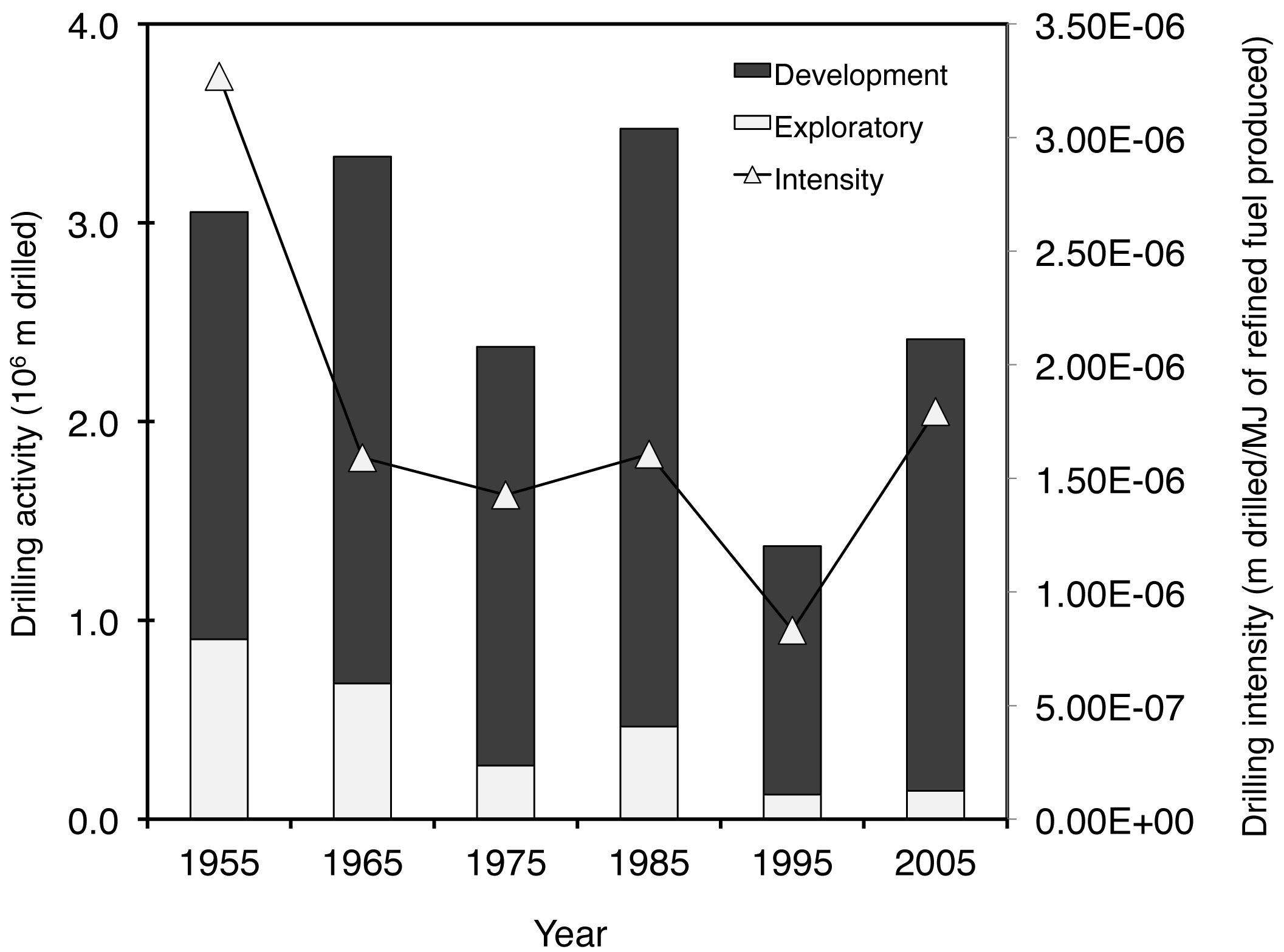
3.3.2. Drilling Energy Use
Drilling activity data are calculated using field-level development drilling and data on exploratory drilling. Dry holes are included in exploratory drilling data. The total energy consumed in drilling is:
All drilling energy is assumed to be provided by diesel-powered drill rigs. Drill rig energy consumption data are difficult to obtain. Using estimates from drilling companies [41,42] and data on fuel consumption in drill rig engines [37], energy consumption in modern oil well drilling was previously estimated as 250 MJ/m (low case) and 400 MJ/m (high case) for shallow wells (1000 m and less) [43].
The amount of time required to drill a well, and consequently the energy consumed, tends to increase exponentially with depth [44]. Using data from modern Canadian well drilling data [45–47] the following relationships between MJ/m and well depth are generated:
Changes in drilling energy intensities over time can only be approximated. Drill rig engine sizes increased by at least a factor of 4 over the modeled time period, from 200–375 kW in 1950 [48, p. 159] to ≥800 kW in 1975 and ≥1500 kW in 2005 [37]. This additional power resulted in faster drilling, but it is unclear if power increases resulted in more energy efficient drilling (on a MJ/m basis).
Improvement in efficiency of diesel engines was slow over the modeled time period. Large marine diesel engines reached efficiencies near present-day efficiencies by the 1950s, with thermal efficiencies of 45% achieved by 1950 [49]. Smaller diesel engine efficiencies lag behind large engine efficiencies: Caterpillar engines for land-based drilling rigs have increased in efficiency from from 0.31 to 0.41 MJ motive power/MJ fuel, lower heating value (LHV) basis over the modeled time period [37,38,48]. All engines compared are Caterpillar drill rig engines. 1955 engines included Caterpillar models D364, D375, D397 [48, p. 174]. The model includes data on D397, as this was the largest engine with ≈ 375 kW output at 1200 rpm. D397 fuel input at its most efficient was interpolated from figures on specification sheet to be 0.42 lb fuel per brake horsepower hour produced [38]. Using cited fuel energy density of 19,000 BTU/lb, this amounts to a technical efficiency of 0.313 MJ motive power per MJ of input diesel (LHV basis). For 1975 and 2005 engines, data from Caterpillar Repower brochure suggest engines of the time were the D399 and 3516 [37,50, Reported fuel consumption rates imply efficiencies of 0.334 and 0.405, LHV basis, respectively, from these engines]. The model interpolates these changes over modeled period, resulting in drilling fuel consumption multipliers of 1.29 in 1955, 1.21 in 1975, and 1.00 in 2005.
Energy costs of cement and steel are included [51]. The methods used are equivalent to those used in a previous analysis of in situ oil shale development [43], with energy intensities of ≈ 19,000 MJ/tonne of steel and 2400 MJ/m3 of cement. Energy consumed in steel and cement manufacture are relatively small compared to direct drilling energy inputs (steel = 1/4, cement = 1/30).
3.3.3. Energy Costs of Lifting
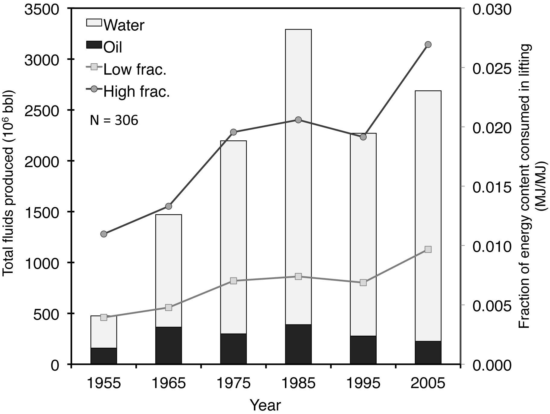
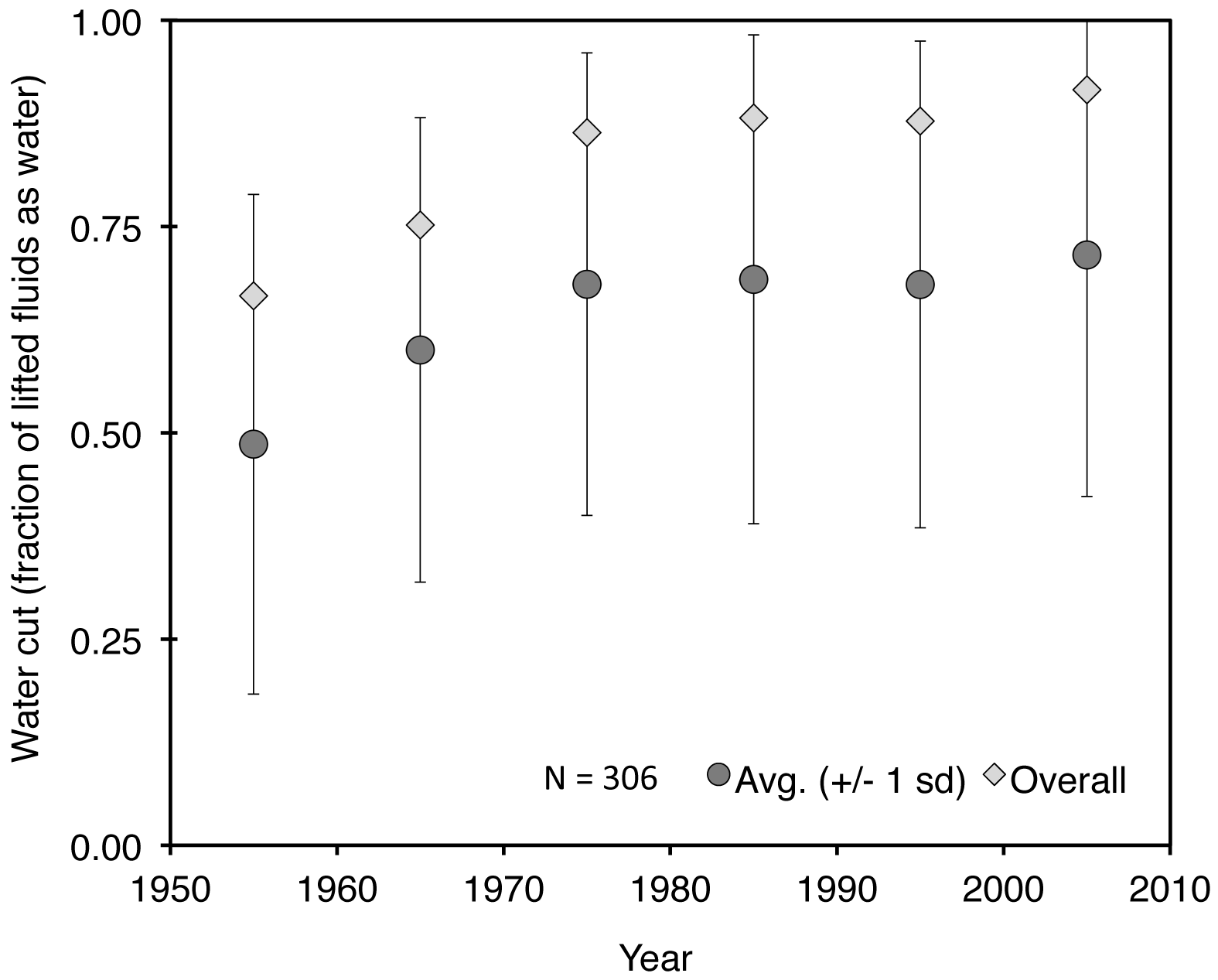
Lifting activity data collected include volumes of fluids lifted per field per year, including oil, water and gas. Oil volumes are converted to masses lifted using the specific gravity of individual fields' oil output. Oil and water lifted over time are plotted in Figures 4 and 5.
Technical efficiencies are calculated assuming pumping is provided by electric-powered sucker-rod pumps (SRPs) [52]. Pumping in California oil fields is in most cases electric, and 80% of oil well pumps are SRPs [52]. Pumping efficiency is determined by mechanical losses, friction in well bores, and electricity generation efficiency The energy requirements of crude oil lifting are derived from a modified version of a pressure drop equation [53]:
The change in kinetic energy (EA) is often neglected, so I ignore it here [53] (Fluids are not moving appreciably faster at the surface than in the wellbore, and kinetic energy quantities are small for observed velocities.) Since data on well pressures by field and time are not available, the model also neglects energy supplied by reservoir pressure drawdown (EP). The model represents losses EF with an efficiency multiplier [54]. SRP efficiency ηpump is the product of mechanical efficiency, ηm, electric motor efficiency, ηt, efficiency of lifting, ηl, and efficiency of electricity generation ηe [54] [55]. So for a given oil field i:
Given that sucker rod pumps are a relatively simple and mature technology, the model assumes no changes in pump efficiency (ηm, ηl) over the modeled time period. Data from EIA are used to calculate ηe, using US average electricity generation efficiency (improves from 26.2% in 1955 to 31.4% in 2005) [39]. Ideally, California-specific electricity efficiencies would be used, but EIA state data are only available to 1990. Data from Ayres et al. are used to calculate changes to electric motor efficiency over time (ηt improves from 79.1% to 90%) [56].
3.3.4. Steam Injection for Thermal Enhanced Oil Recovery
Steam injection activity data were first reported in 1966, so 1966 data are used as a proxy for 1965 steam injection values. Total volumes of steam injected are multiplied by the energy requirements per barrel of steam generated. Steam is modeled as requiring 1990–2330 MJ/m3 (0.3–0.35 mmBtu/bbl) of cold water equivalent steam (Low case-High case) [57]. All steam is assumed to be generated in 75–85% efficient (High case-Low case, LHV basis) once-through steam generators [58], except for steam generated with cogeneration systems (see below). Due to lack of data suggesting otherwise, the model assumes that efficiency of steam generation stays constant across the modeled time period. For a more thorough analysis of the emissions and efficiency of TEOR, see work by Brandt and Unnasch [59].
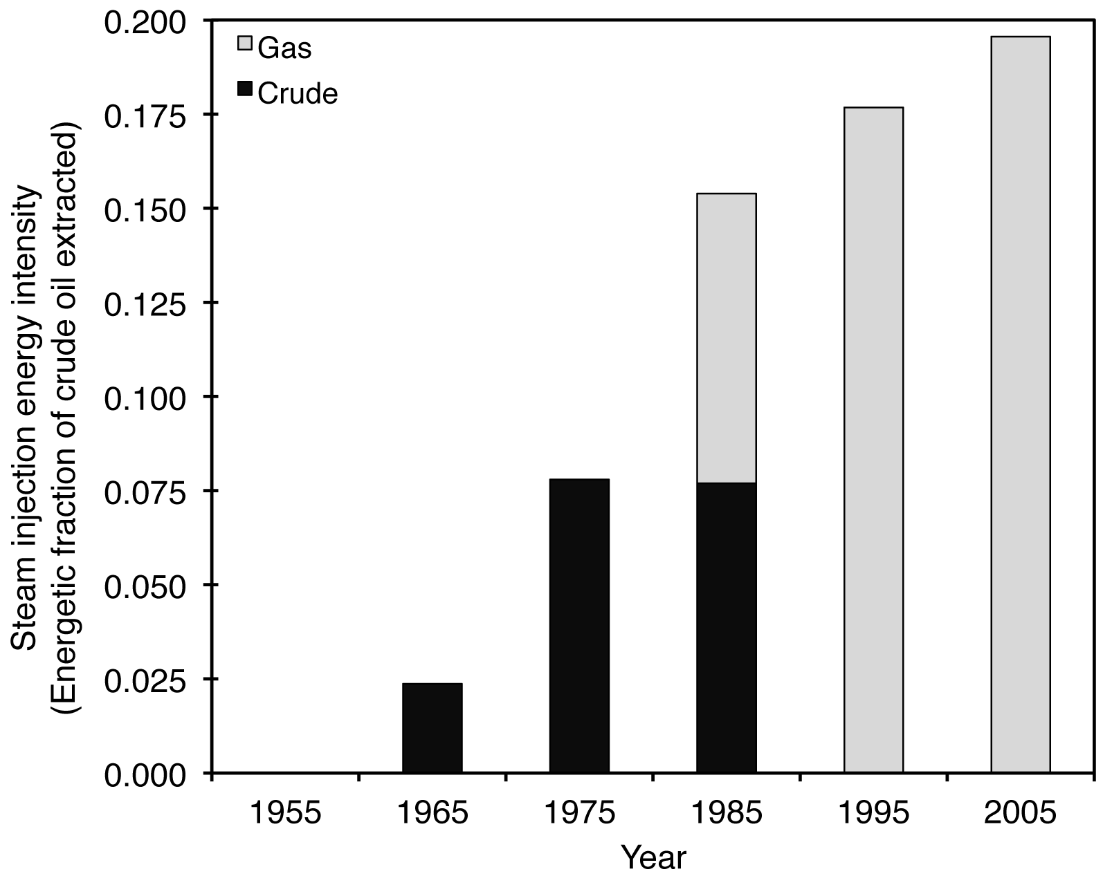
The energy requirements of steam production are normalized by the total crude energy produced and are plotted in Figure 6. This figure shows that in recent decades, over 15% of the equivalent energy content of produced crude in California has been used for steam generation. This significant increase in the energy consumed in steam generation reduces both the NER and (once external natural gas begins to be consumed in the 1980s) the EER. No data are reported on steam production fuel by year, so the fraction fueled with crude oil and natural gas is estimated from the history of industry regulation above: all steam is assumed to be produced with produced oil until 1985, when 50% is assumed to be produced with natural gas. From 1995 onward, all steam is assumed produced with natural gas (see Figure 7 for data on expansion of natural gas fired cogeneration).
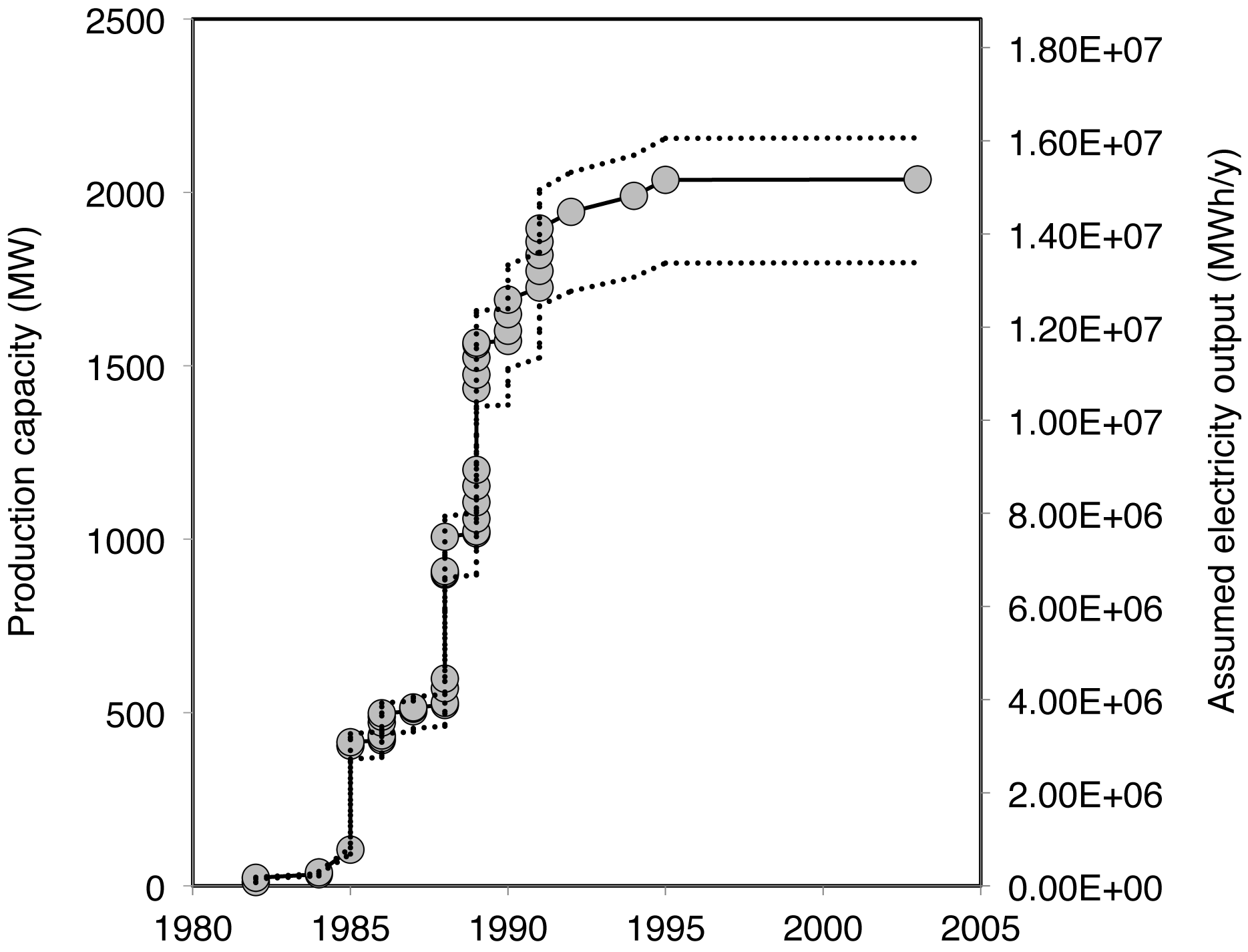
In the 1980s, as the transition to natural gas was occurring, oil producers added cogeneration facilities. This expansion of TEOR cogeneration capacity is shown in Figure 7. For inclusion in total EROI and EER figures, electricity flow Ff,e– is weighted by a factor of 3 to account for its approximate 33% conversion efficiency from primary energy.
Cogeneration efficiency and steam/power ratios are taken from Brandt and Unnasch [59], given by cogeneration low and cogeneration high cases. These efficiencies account for the larger natural gas demand due to co-production of electricity (e.g., only ≈ 45% of thermal energy is imparted to steam). This additional natural gas demand offsets some of the energetic benefits of co-producing electricity.
3.4. Refining Energy Inputs
The model uses a linear function for refining energy consumption variation with crude specific gravity, derived from results of Keesom et al. [61], who modeled refinery energy consumption for 11 crude streams ranging from 0.842 to 1.011 specific gravity. Linear functions are fit to reported internal and external energy inputs to refining as a function of crude volumes, arriving at an overall equation for crude refining energy use:
No data were found on the time-varying efficiency of oil refining. In the absence of data, the model assume refinery energy consumption per unit of energetic throughput decreased by 2.5% per 10 year period in the Low case and 5% per 10 year period in the High case. Thus, a refinery consumption multiplier is included in the model (in the High case equals 1.25 in 1955, 1.2 in 1965, etc.).
4. Results and Discussion
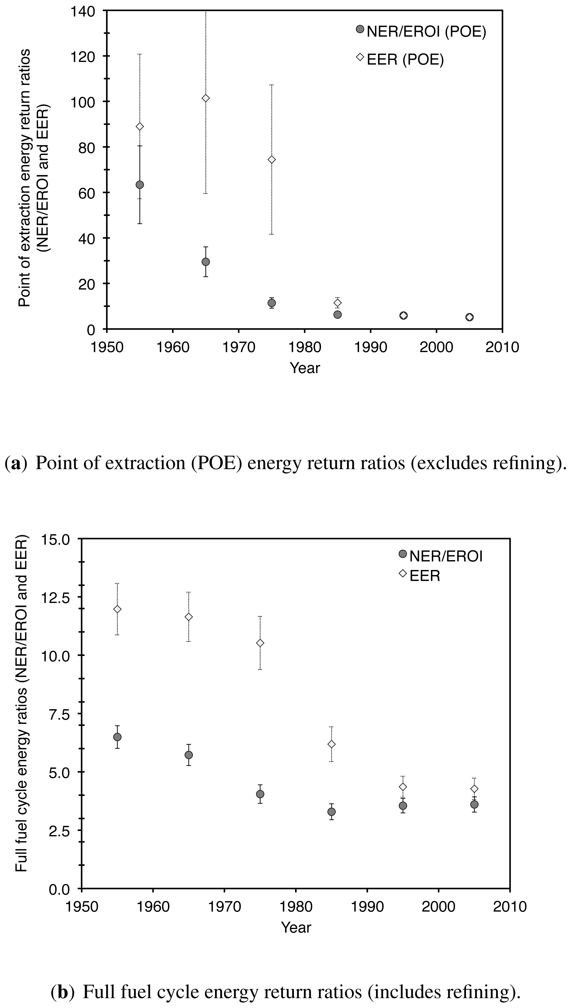
Energy inputs and outputs for California oil production are presented in Table 4 for the low case (in PJ per year). Calculated values of NER and EER are plotted in Figure 8. Error bars represent low and high case assumptions, markers represent average of low and high cases. Point of extraction EROI drops significantly over the modeled time period, from over 60 to ≈ 5. Also, full fuel cycle NER/EROI declined from ≈ 6.5 to 3.5, while EER dropped from 12 to 4.25. Both of these trends illustrate the decreasing energetic returns from oil extraction as depletion progresses. This should be expected given the trends observed above (e.g., increasing water cut, increasing fraction of energy consumed in steam generation).
Note the significant difference between values measured at the point of extraction (POE) and values measured over the entire fuel cycle. This divergence is due to the fact that refining is a large and fairly consistent consumptive sector, which reduces significantly the ratio between the numerator (outputs) and the denominator (total consumption).
These trends reflect on the balance between quality factors and technical efficiencies, as discussed above. As the quality factors declined in favorability in the California oil industry (e.g., more water must be lifted for each unit of oil produced), the increase in technical efficiencies did not fully compensate for these reductions in quality. This trend caused the energetic returns to oil extraction to decline significantly over the modeled time period. The largest portion of this effect is due to energy consumption for TEOR, seen in xc1 and most of xe1 in Table 4.
Figure 8 shows a closing of the gap between NER and EER beginning in the mid-1980s. This is due to changing of the primary energy source for California TEOR steam production. Originally, steam for EOR was generated using produced heavy crude. Producers switched to natural gas for generating steam, thus the internal energy use xc1 drops significantly by 1985, reducing the gap between NER and EER. TEOR ceased to be a largely self-fueled process at this time.
Useful information can be obtained by comparing the values of NER and EER for a given process. Such comparisons illustrate how much of a conversion and extraction process is self-fueled. For example, in previous studies of oil shale development in the Green River formation of Colorado, Brandt [43,63] found that EER and NER varied greatly for in situ and mine-and-retort oil shale extraction schemes. This is because the oil shale extraction processes studied were fueled primarily by the shale inputs to the retorting process. Similar considerations applied to the largely self-fueled early TEOR operations. These operations were less energy efficient, but because only produced crude was being consumed, this did not result in an additional draw on other resources such as natural gas. This self use reduces the endowment of oil and the net output per unit of capital investment, but will not affect other energy sectors appreciably. Self use also results in environmental impacts (e.g., GHGs per unit of energy output).
The uncertainty in model results is significant. EROI values actually achieved in the California oil industry over time are fundamentally unobservable: many of the required data inputs are not publicly available or were likely even lost over time due to neglect. This lack of data causes fundamental difficulties in assessing the uncertainty. One conclusion is that this uncertainty is uneven in the above model functions: detailed operations data are available at the field level in CDC-DOGGR statistics, while little data are available on technical efficiencies over time. Again, these data were not required to be reported by regulatory bodies and were therefore never publicly documented.
Despite these uncertainties, this type of analysis has significant value. Because the model relies on bottom-up data, such as m3 of water lifted, additional understanding of depletion effects can be generated compared to top-down EROI assessments based on aggregated economic data. In theory, this allows diagnosis of the most important effects of depletion, and industry effectiveness in responding to these depletion impacts.
The global impacts of these forms of depletion on the energy efficiency and environmental impacts of oil extraction are still poorly understood. At this time of rapid expansion of low-quality oil resources such as the Canadian tar sands, this is a troublesome gap in knowledge. Given the size and energy intensity of oil extraction and refining operations, the impacts of such changes on global environmental impacts are likely large.


| Field | Pre-steam | Post-steam | ||||
|---|---|---|---|---|---|---|
| Year | Prod. (106 m3) | Prod. (Mbbl) | Year | Prod. (106 m3) | Prod. (Mbbl) | |
| Kern River | 1904 | 2.73 | 17.2 | 1985 | 8.20 | 51.6 |
| Midway-Sunset | 1914 | 5.46 | 34.4 | 1991 | 9.74 | 61.3 |
| South Belridge | 1945 | 0.73 | 4.6 | 1987 | 10.11 | 63.56 |
| Name | Tight system boundaries | Loose system boundaries | Characteristics |
|---|---|---|---|
| NER/EROI | Net energy ratio. Ratio of outputs to total energy consumed in production. All x flows are included because ratio includes consumption of self produced energy. EROI provides understanding of overall efficiency of process and is proportional to impacts associated with energy use (e.g., environmental impacts). | ||
| NER/EROI (POE) | Same | Net energy ratio at point of extraction. As above, except calculated at the point of crude oil extraction rather than on refined fuel basis. | |
| EER | External energy ratio.a Refined energy provided to non-energy sectors of the economy, divided by the energy input from external energy system. Indicator of ability of process to increase energy supply to society. | ||
| EER (POE) | Same | External energy ratio calculated at the point of extraction. As above, except calculated at the point of crude oil extraction rather than on refined fuel basis. |
aThis quantity has also been called External Net Energy Ratio (ENER) [25].
| Data input | Source | Scale | Years |
|---|---|---|---|
| Oil production | [36] | 306 fields | 1955–2005 |
| Water production | [36] | 306 fields | 1955–2005 |
| Development wells drilled | [36] | 306 fields | 1955–2005 |
| Exploratory wells drilled | [36] | State-wide | 1955–2005 |
| Steam injection | [36] | 306 fields | 1965–2005 |
| API gravity | [11] | Pool/field | NA |
| Depth | [11] | Pool/field | NA |
| Drill rig efficiency | [37,38] | 3 reported efficiencies | ≈ 1950, 1975, 2005 |
| Electricity efficiency | [39] | US average efficiency | 1955–2005 |
| Flow | 1955 | 1965 | 1975 | 1985 | 1995 | 2005 |
|---|---|---|---|---|---|---|
| Fi | 1011 | 2298 | 1928 | 2488 | 1778 | 1446 |
| Fc | 1011 | 2256 | 1814 | 2342 | 1778 | 1446 |
| Fr | 943 | 2110 | 1677 | 2171 | 1654 | 1346 |
| Ff,oil | 942 | 2109 | 1676 | 2170 | 1654 | 1345 |
| Ff,e– | 0 | 0 | 0 | 12 | 58 | 58 |
| Ff,gas | 208 | 340 | 210 | 263 | 177 | 230 |
| xe1 | 7 | 15 | 16 | 169 | 264 | 243 |
| xr1 | 1 | 1 | 0 | 1 | 0 | 0 |
| xc1 | 0 | 41 | 114 | 146 | 0 | 0 |
| Wc1 | 4 | 6 | 1 | 0 | 0 | 0 |
| xe2 | 65 | 148 | 124 | 160 | 114 | 93 |
| xr2 | 0 | 0 | 0 | 0 | 0 | 0 |
| xc2 | 68 | 147 | 137 | 171 | 124 | 100 |
| xinc2 | 6 | 13 | 11 | 14 | 10 | 8 |
Acknowledgments
Charles Hall and Richard Sears provided detailed comments on the methods used here. Bryan Sell and Jon Freise provided numerous helpful comments on the manuscript, as well as additional data on drilling energy intensity. Members of the Antique Caterpillar Machinery Owners Club generously provided historical technical specifications for Caterpillar drill rig engines from the 1950s and 1970s. Additionally, helpful comments on an earlier version of this work were provided by Tad Patzek, Alex Farrell and Richard Norgaard at UC Berkeley.
References
- Farrell, A.E.; Brandt, A.R. Risks of the oil transition. Environ. Res. Lett. 2006, 1, 014004. [Google Scholar]
- Brandt, A.R. Testing hubbert. Energy Policy 2007, 35, 3074–3088. [Google Scholar]
- Deffeyes, K.S. Hubbert's Peak: The Impending World Oil Shortage; Princeton University Press: Princeton, NJ, USA, 2001; p. 208. [Google Scholar]
- Campbell, C.J.; Laherrere, J. The end of cheap oil. Sci. Am. 1998, 278, 78–83. [Google Scholar]
- Hall, C.A.S.; Cleveland, C.J. Petroleum drilling and production in the United States: Yield per effort and net energy analysis. Science 1981, 211, 576–579. [Google Scholar]
- Cleveland, C.J. Net energy from the extraction of oil and gas in the United States. Energy 2005, 30, 769–782. [Google Scholar]
- Rintoul, W. Spudding in: Recollections of Pioneer Days in the California Oil Fields; California Historical Society: San Francisco, CA, USA, 1976. [Google Scholar]
- Rintoul, W. Drilling through Time: 75 Years with California's Division of Oil and Gas; California Dept. of Conservation Division of Oil and Gas: Sacramento, CA, USA, 1990. [Google Scholar]
- API. Petroleum Facts and Figures: Centennial Edition; American Petroleum Institute: New York, NY, USA, 1959. [Google Scholar]
- API. Basic Petroleum Data Book: Petroleum Industry Statistics. In Basic Petroleum Data Book; American Petroleum Institute: Washington, DC, USA, 2004; p. 24. [Google Scholar]
- CDC-DOGGR. California Oil and Gas Fields, Volumes I–III; Technical report; California Department of Conversation, Division of Oil, Gas, and Geothermal Resources: Sacramento, CA, USA, 1982–1998. [Google Scholar]
- Rintoul, W. Oildorado: Boom Times on the West Side; Valley Publishers: Fresno, CA, USA, 1978. [Google Scholar]
- Rintoul, W. Drilling Ahead: Tapping California's Richest Oil Fields, 1st ed.; Valley Publishers: Santa Cruz, CA, USA, 1981. [Google Scholar]
- CDC-DOGGR. Summary of Operations: California Oil Fields; Technical report; California Department of Conservation, Division of Oil and Gas, and Geothermal Resources: Sacramento, CA, USA, 1966. [Google Scholar]
- CCCOGP. Annual Review of California Oil and Gas Production; Technical report; Conservation Committee of California Oil and Gas Producers: Bakersfield, CA, USA, 1994. [Google Scholar]
- Dennison, W.J.; Taback, H.; Parker, N. Emissions Characteristics of Crude Oil Production Operations in California; Consultant report KVB72-5810-1309ES; California Air Resources Board: Sacramento, CA, USA, 1983. [Google Scholar]
- Norton, J.F. A Report to the California Energy Commission: The Options for Increasing California Heavy Oil Production: Final Report; Radian Corporation: Sacramento, CA, USA, 1981. [Google Scholar]
- Henwood, M.I. Feasibility and Economics of Cogeneration in California's Thermal Enhanced Oil Recovery Operations; California Energy Commission, Assessment Division: Sacramento, CA, USA, 1978. [Google Scholar]
- CDC-DOGGR. 2003 Annual Report of the State Oil & Gas Supervisor; Technical report; California Department of Conservation, Division of Oil, Gas and Geothermal Resources: Sacramento, CA, USA, 2004. [Google Scholar]
- Production is lightly taxed in California (e.g., no mineral severance tax), the reduction in California oil production is not likely a major driver of California's recent budget difficulties. The production decline since peak production amounts to ≈ 200 Mbbl/y, which if valued at 100 $/bbl would equal ≈ 1% of California's total economic output.
- CDC-DOGGR. 2008 Annual Report of the State Oil & Gas Supervisor; Technical report; California Department of Conservation, Division of Oil, Gas and Geothermal Resources: Sacramento, CA, USA, 2009. [Google Scholar]
- ISO. ISO 14040: Environmental Management—Life Cycle Assessment—Principles and Framework; International Organization for Standardization: Geneva, Switzerland, 2006. [Google Scholar]
- ISO. ISO 14044: Environmental Management—Life Cycle Assessment—Requirements and Guidelines; International Organization for Standardization: Geneva, Switzerland, 2006. [Google Scholar]
- Herendeen, R.A. Net Energy Analysis: Concepts and Methods. In Encyclopedia of Energy; Cleveland, C.J., Ed.; Elsevier: Amsterdam, The Netherlands, 2004; Volume 4, pp. 283–289. [Google Scholar]
- CERI. Net Energy Analysis: An Energy Balance Study of Fossil Fuel Resources; Technical report; Colorado Energy Research Institute: Golden, CO, USA, 1976. [Google Scholar]
- Pehnt, M. Dynamic Life Cycle Assessment (LCA) of renewable energy technologies. Renew. Energy 2006, 31, 55–71. [Google Scholar]
- Levasseur, A.; Lesage, P.; Margni, M.; Descheacnes, L.; Samson, R. Considering Time in LCA: Dynamic LCA and its application to global warming impact assessments. Environ. Sci. Technol. 2010, 44, 3169–3174. [Google Scholar]
- Mendivil, R.; Fischer, U.; Hirao, M.; Hungerbuhler, K. A new LCA methodology of technology evolution (TE-LCA) and is application to the production of ammonia (1950–2000). Int. J. Life Cycle Assess. 2006, 11, 98–105. [Google Scholar]
- Farrell, A.; Plevin, R.J.; Turner, B.T.; Jones, A.D.; O'Hare, M.; Kammen, D.M. Ethanol can contribute to energy and environmenal goals. Science 2006, 311, 506–508. [Google Scholar]
- Cleveland, C.J. Energy quality and energy surplus in the extraction of fossil fuels in the US. Ecol. Econ. 1992, 1992, 139–162. [Google Scholar]
- Gever, J. Beyond Oil: The Threat to Food and Fuel in the coming Decades, 3rd ed.; University Press of Colorado: Niwot, CO, USA, 1986. [Google Scholar]
- Hall, C.A.S.; Cleveland, C.J.; Kaufmann, R. Energy and Resource Quality: The Ecology of the Economic Process; Wiley: New York, NY, USA, 1986. [Google Scholar]
- Spitzley and Keolian outline more than 10 energy return ratios that have been used previously. These ratios differ in system boundaries included, in the quantity of interest, and in the inclusion or exclusion of various energy types (e.g., fossil energy return ratios that measure the leveraging of fossil energy streams in renewable energy systems). In many published studies, authors fail to specify exactly which energy return ratio is used.
- Spitzley, D.V.; Keoleian, G. Life Cycle Environmental and Economic Assessment of Willow Biomass Electricity: A Comparison with other Renewable and Non-Renewable Sources; Technical Report CSS04-05R; University of Michigan: Ann Arbor, MI, USA, 2004. [Google Scholar]
- Large amounts of data are available from the California Department of Conservation—Department of Oil, Gas, and Geothermal Resources (CDC-DOGGR). Databases contain well-level information from the late 1970s to the present, and field-level data are available in annual reports dating to 1915.
- CDC-DOGGR. Summary of Operations and Annual Report of the State Oil & Gas Supervisor (Various); Technical report; California Department of Conservation, Division of Oil, Gas and Geothermal Resources: Sacramento, CA, USA, 1955–2005. [Google Scholar]
- Caterpillar. Drilling rig repower. Brochure, Caterpillar Inc.: Peoria, IL, USA, 2003. http://catoilandgas.cat.com/cda/files/823409/7/LEDW3153.pdf. [Google Scholar]
- Caterpillar. Caterpillar D397 Twelve Cylinder Specification Sheet; (Date illegible, approximately 1950).
- EIA. Electric Power Annual 2007; Technical report; Energy Information Administration: Washington, DC, USA, 2009. [Google Scholar]
- Schmidt, P.F. Fuel Oil Manual, 4th ed.; Industrial Press: New York, NY, USA, 1985. [Google Scholar]
- Cheyenne Drilling Inc. Personal communication with staff of Cheyenne Drilling on energy consumption during drilling; 2006. [Google Scholar]
- Cheyenne Drilling Inc. Drilling rig information, rig 1; Web page; Cheyenne Drilling, 2006. [Google Scholar]
- Brandt, A.R. Converting oil shale to liquid fuels: Energy inputs and greenhouse gas emissions of the Shell in situ conversion process. Environ. Sci. Technol. 2008, 42, 7489–7495. [Google Scholar]
- Azar, J.; Robello, G. Drilling Engineering; PennWell Publishers: Tulsa, OK, USA, 2007. [Google Scholar]
- PSAC. 2001/2002 Well Cost Study; Technical report; Petroleum Services Association of Canada: Calgary, AB, Canada, 2000. [Google Scholar]
- PSAC. 2002 Well Cost Study; Technical report; Petroleum Services Association of Canada: Calgary, AB, Canada, 2001. [Google Scholar]
- PSAC. 2005 Well Cost Study; Technical report; Petroleum Services Association of Canada: Calgary, AB, Canada, 2005. [Google Scholar]
- Gow, S. Roughnecks, Rock Bits and Rigs: The Evolution of Oil Well Drilling Technology in Alberta 1883–1970; University of Calgary Press: Calgary, AB, Canada, 2005. [Google Scholar]
- Smil, V. Prime Movers of Globalization: The History and Impact of Diesel Engines and Gas Turbines; The MIT Press: Cambridge, MA, USA, 2010. [Google Scholar]
- Caterpillar Inc. Caterpillar D399 Marine Generator Set - Technical Specifications. 1980. https://marine.cat.com/cda/files/1014636/7/Spec+Sheet+-+Cat+D399+Genset.pdf. [Google Scholar]
- Horvath, A. Construction materials and the environment. Annu. Rev. Environ. Resour. 2004, 29, 181–204. [Google Scholar]
- Brennan, J.R.; Vance, W.M. Section 9.17 - Oil Wells. In Pump Handbook, 3rd ed.; Karassik, I.J., Messina, J.P., Cooper, P., Heald, C.C., Eds.; McGraw Hill: New York, NY, USA, 2001. [Google Scholar]
- Lyons, W.C.; Plisga, G.J. Standard Handbook of Petroleum and Natural Gas Engineering, 2nd ed.; Gulf Professional Imprint of Elsevier: Burlington, MA, USA, 2005. [Google Scholar]
- Takacs, G. Sucker-Rod Pumping Manual; PennWell Books: Tulsa, OK, USA, 2003. [Google Scholar]
- Cited values of ηt ranges from 85% to 93%, while ηl ranges from 38% to 94% [54]. The lowest values were due to rubbing of the pump string against well casing in deviated wells [54]. I assume ηm ranges from 80-90%.
- Ayres, R.U.; Ayres, L.W.; Pokrovsky, V. On the efficiency of US electricity usage since 1900. Energy 2005, 30, 1092–1145. [Google Scholar]
- Green, D.W.; Willhite, G.P. Enhanced Oil Recovery; Henry L. Doherty Memorial Fund of AIME, Society of Petroleum Engineers: Richardson, TX, USA, 1998. [Google Scholar]
- Burger, J.; Sourieau, P.; Combarnous, M. Thermal Methods of Oil Recovery, 3rd ed.; Editions Technip, Gulf Publishing Company: Houston, TX, USA, 1985. [Google Scholar]
- Brandt, A.R.; Unnasch, S. Energy intensity and greenhouse gas emissions from California thermal enhanced oil recovery. Energy & Fuels 2010, 24, 4581–4589. [Google Scholar]
- CDC-DOGGR. Annual Report of the State Oil & Gas Supervisor; Technical report; California Department of Conservation, Division of Oil, Gas and Geothermal Resources: Sacramento, CA, USA, 2005. [Google Scholar]
- Keesom, W.; Unnasch, S.; Moretta, J. Life Cycle Assessment Comparison of North American and Imported Crudes; Technical report; Jacobs Consultancy and Life Cycle Associates for Alberta Energy Resources Institute: Chicago, IL, 2009. [Google Scholar]
- Wang, M.Q. Estimation of Energy Efficiencies of US Petroleum Refineries (Plus Associated Spreadsheet); Technical report; Center for Transportation Research, Argonne National Laboratory: Argonne, IL, USA, 2008. [Google Scholar]
- Brandt, A.R. Converting oil shale to liquid fuels with the Alberta taciuk processor: Energy inputs and greenhouse gas emissions. Energy Fuels 2009, 23, 6253–6258. [Google Scholar]
© 2011 by the author; licensee MDPI, Basel, Switzerland. This article is an open access article distributed under the terms and conditions of the Creative Commons Attribution license (http://creativecommons.org/licenses/by/3.0/.)
Share and Cite
Brandt, A.R. Oil Depletion and the Energy Efficiency of Oil Production: The Case of California. Sustainability 2011, 3, 1833-1854. https://doi.org/10.3390/su3101833
Brandt AR. Oil Depletion and the Energy Efficiency of Oil Production: The Case of California. Sustainability. 2011; 3(10):1833-1854. https://doi.org/10.3390/su3101833
Chicago/Turabian StyleBrandt, Adam R. 2011. "Oil Depletion and the Energy Efficiency of Oil Production: The Case of California" Sustainability 3, no. 10: 1833-1854. https://doi.org/10.3390/su3101833