The EROI of Conventional Canadian Natural Gas Production

Abstract

Canada was the world's third largest natural gas producer in 2008, with 98% of its gas being produced by conventional, tight gas, and coal bed methane wells in Western Canada. Natural gas production in Western Canada peaked in 2001 and remained nearly flat until 2006 despite more than quadrupling the drilling rate. Canada seems to be one of many counter examples to the idea that oil and gas production can rise with sufficient investment. This study calculated the Energy Return on Energy Invested and Net Energy of conventional natural gas and oil production in Western Canada by a variety of methods to explore the energy dynamics of the peaking process. All these methods show a downward trend in EROI during the last decade. Natural gas EROI fell from 38:1 in 1993 to 15:1 at the peak of drilling in 2005. The drilling intensity for natural gas was so high that net energy delivered to society peaked in 2000–2002, while production did not peak until 2006. The industry consumed all the extra energy it delivered to maintain the high drilling effort. The inability of a region to increase net energy may be the best definition of peak production. This increase in energy consumption reduces the total energy provided to society and acts as a contracting pressure on the overall economy as the industry consumes greater quantities of labor, steel, concrete and fuel. It appears that energy production from conventional oil and gas in Western Canada has peaked and entered permanent decline.

1. Introduction

At the start of the 21st century we have a lot of pressing questions about our future energy supply: Can the world maintain its oil production plateau? Can natural gas production grow to replace coal and oil? Is it physically possible to grow the economy using renewable energy sources or even transition to renewable energy sources?

What ties these questions together is a concept called net energy. It takes an investment of energy (in the form of fuel, steel, labor, and more) to produce energy. The net energy is the amount of surplus after this investment has been paid. This surplus is the energy available to operate the rest of the economy. All of these questions may be asked in a simpler form: Can we do X and still maintain or grow the net energy supply? Thus, insight gained from understanding the energy production of fossil fuels may transition to understanding of the growth (or decline) of renewable energy sources.

Canada's oil and natural gas industry makes an interesting case study for net energy analysis. The country is a very large petroleum producer and was the world's third largest natural gas producer in 2008 [1] and most of that production comes from the onshore Western Canadian Sedimentary Basin (WCSB). It went through a peak in oil production in the 1970s and, despite an increase in drilling, the country could not return to peak rates. Most recently, natural gas production fell from an eight-year plateau despite a 300% increase in the rate of drilling and an even greater increase in investment.

A net energy analysis of Canadian conventional oil and natural gas provides several things: Firstly, it is a measurement of current conditions. How much net energy is being produced now and what is the trend? Secondly, it provides insight into the net energy dynamics of the production growth, peak/plateau, and decline for oil and natural gas production. Thirdly, it gives some indication of what net energy levels are needed for an energy system to grow and below which levels cause a peak or decline in the energy system.

This paper will calculate the net energy for oil and, most importantly, natural gas production in the WCSB using publically available data on a fine grained yearly basis. Three methods will be used: The simplest will calculate a net energy return for oil and natural gas back to 1947 for historical reference and to encompass the 1973 oil peak. Two others will calculate the yearly net energy of natural gas production from 1993 onward: the first using publically available statistical data and the second using natural gas cost per GJ estimates created periodically by the Canadian National Energy Board (NEB) for forecasting purposes. The results will then be examined to see what conclusions can be drawn about the current state of oil and gas net energy, the energy dynamics of the production peaks, and what these results might mean for non-Canadian natural gas production and growth of energy sources in general.

1.1. Net Energy and the Economy

It takes energy to produce energy. For natural gas and oil production, energy is consumed as fuel to drive drilling rigs and other vehicles, energy to make the steel in drill and casing pipe, energy to heat the homes of the workers and provide them with food. These energy expenditures make up the cost of producing energy. Net energy is the surplus energy after these costs have been paid. The equation for net energy is shown in Equation 1.

$$\mathit{\text{Net}}\mathit{\text{Energy}}=\mathit{\text{Energy}}\mathit{\text{Outputs}}-\mathit{\text{Energy}}\mathit{\text{Inputs}}$$

(1)

This is often expressed as a ratio called Energy Return on energy Invested:

$$\mathit{\text{EROI}}=\frac{\mathit{\text{Energy}}\mathit{\text{Outputs}}}{\mathit{\text{Energy}}\mathit{\text{Inputs}}}$$

(2)

The net energy is the energy available for powering the economy. Energy supply and demand are intrinsically linked by more than the price, because the supply is creating (powering) the demand. This point is crucial for understanding the net energy dynamics of a peak in oil and gas production.

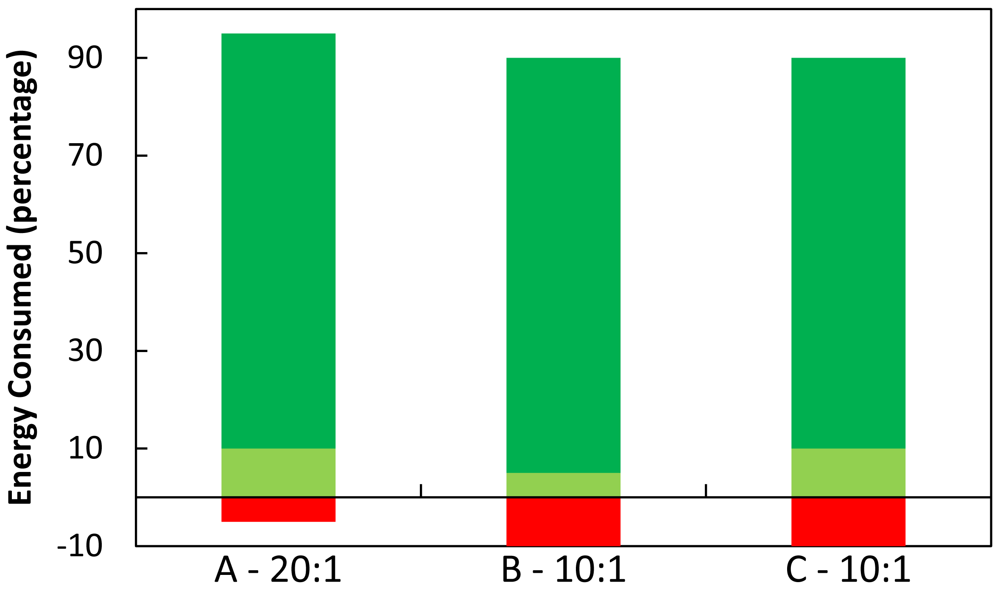
High energy prices cause recessions [2-5] and Figure 1, a simple schematic of net energy adapted from [6], helps illustrate the reason for this from a net energy perspective. The red represents the energy needed to produce energy. The dark green is the energy consumed refining, transporting and using the energy. The light green is the energy surplus available to operate, maintain and possibly grow the economy. Column A represents the economy before the cost of energy rises, and column B is the economy afterwards.

As costs rise, the energy sector makes a huge increase in its demand for labor, steel, fuel, etc. from society at large, shown by a large increase in the red area. But at the same time, the energy sector is providing no additional energy that is needed to create that extra steel, supply the fuel, or support the labor. Society must then cannibalize other sectors to supply the demands of the energy sector and the non-energy economy is seen to contract. This non-energy sector contraction would then cause a collapse in demand for energy, and returning society to somewhere between A and B.

To help formalize this example, assume Figure 1 shows a theoretical energy source supplying 1 Giga Joule (GJ) of energy. The three columns show three different net energy conditions. Column A shows an energy supply that requires 5% of the gross energy as input energy. It has an EROI of 20:1 and a net energy of 95%.

Column B shows the same energy source, but where the cost of producing energy has doubled to consume 10% of the gross energy supply. It has an EROI of 10:1 and a net energy of 90%. The transport, refining, and end use efficiency remain the same and so the final surplus has contracted.

Column C represents a society that has adapted to the lower EROI energy source by improving efficiency of use and the surplus has returned. The more efficient a society, the lower the net energy supply it may subsist upon. This last point will be important when examining the difference between the peaks in oil and natural gas.

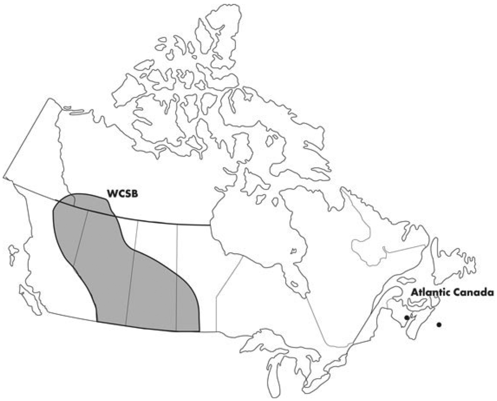
1.2. Background on the Western Canadian Sedimentary Basin

Western Canada produced 98% of Canada's natural gas in 2009 with the majority of that coming from the Western Canadian Sedimentary Basin (WCSB) that underlies most of Alberta, parts of British Columbia, Saskatchewan and the Northwest Territories [7].

This paper focuses on conventional natural gas, tight natural gas (gas in a low porosity geologic formation that must be liberated via artificial fracturing) and conventional oil production. Western Canadian natural gas production is still largely conventional and so makes a good area of study. In 2008, 55% of marketed natural gas was conventional gas from gas wells, 32% was tight gas, 8% was solution gas from oil wells, 5% coal bed methane (non-conventional), and less than 1% was shale gas [9,10].

The Canadian Gas Potential Committee in 2005 estimated that the WCSB contains 71% of the conventional gas endowment of Canada and that of an original 278 Tcf of marketable natural gas (technically and economically recoverable) 143 Tcf remain [11]. They note: “The majority of the large gas pools have been discovered and a significant portion of the discovered reserves has been produced” and further “62% of the undiscovered potential occurs in 21,100 pools larger than 1 Bcf OGIP. The remaining 38% of the undiscovered potential occurs in approximately 470,000 pools each containing less than 1 Bcf”. To put this in context, the petroleum industry has drilled less than 200,000 natural gas wells from 1947 to 2009 [7], and so will require at least a doubling of drilling effort to reach at last half of the marketable natural gas.

2. Results and Discussion

2.1. Method One: EROI and Net Energy of Western Canadian Oil and Gas Production

The Canadian Association of Petroleum Producers (CAPP) maintains records of oil and gas production and expenditures going back to 1947. In theory it is simple to calculate net energy and EROI from this public data. Energy output equals the total production volumes of each hydrocarbon produced in a given year (conventional oil, natural gas, natural gas liquids), which is converted to heat energy equivalents, and measured in Giga Joules. The energy input side is more difficult as the public data for expenditures is recorded only in Canadian $ per year and not in energy. An energy intensity factor is used to convert the dollar expenditures into energy. This factor is calculated from Energy Input Output—Life Cycle Analysis as explained in Section 3 methods. Equation 3 shows the final form:

$$\mathit{\text{Net}}\mathit{\text{Energy}}(J)=\mathit{\text{Heat}}\mathit{\text{Energy}}\mathit{\text{Output}}(J)-(\$*\mathit{\text{Energy}}\mathit{\text{Intensity}}(\frac{J}{\$})$$

(3)

As the energy intensity factor includes wages paid to labor, but energy inputs are not quality corrected, the results are equivalent to EROI_society and not the EROI_Standard [12]. EROI_Standard corrects the input energy for quality but excludes labor costs. The energy intensity factor was 24 MJ/$(U.S. 2002) and all expenditures were inflation corrected and converted to U.S. dollars. While the focus of this paper is on natural gas production, this result provides a historical time line to compare with the more limited time series for natural gas only. The results are first plotted as gross energy and net energy alongside the meters drilled per year as in Figure 4.

The time period from 1947 to 1956 showed rising production along with a rising drilling rate. From 1956 to 1973 production rose despite no corresponding rise in drilling. From 1973 to 1985 production fell despite a rise in drilling effort. The increased drilling rates were unable to increase gross energy and actually drove down net energy during this period.

In the mid-1980s, energy production once again rose with a falling drilling rate. That trend reversed to rising production with increased drilling. Then, in the year 2000, the petroleum industry showed an initial peak in gross and net energy (see

Table 1. Annual gross and net energy production of oil, gas, and natural gas liquids.

Year	Gross Energy Production (1 e9 GJ)	Net Energy Production (1 e9 GJ)	Industry Expenditures (1 e9 U.S.$ 2002)	Energy Invested via 24 MJ/$ (1 e6 GJ)	EROI	Oil & Gas Meters Drilled (1 e6)
1993	8.74	8.53	$8.8	212	41	10.80
1994	9.31	9.03	$11.7	280	33	13.97
1995	9.69	9.42	$11.2	269	36	12.69
1996	10.06	9.78	$11.5	275	37	15.35
1997	10.22	9.87	$14.5	347	29	19.33
1998	10.26	9.96	$12.7	304	34	12.58
1999	10.25	9.98	$11.2	269	38	13.63
2000	10.38	10.02	$14.8	356	29	19.44
2001	10.30	9.89	$17.0	409	25	20.08
2002	10.14	9.78	$15.0	361	28	17.07
2003	9.83	9.41	$17.8	428	23	22.60
2004	9.95	9.46	$20.1	483	21	24.61
2005	9.89	9.30	$24.7	592	17	29.86
2006	9.90	9.25	$27.3	656	15	28.42
2007	9.74	9.17	$23.8	571	17	21.53
2008	9.39	8.80	$24.7	592	16	21.43
2009	8.82	8.37	$18.6	446	20	12.52

). The increases in drilling effort that happened after 2000 were unable to increase production and actually drove down net energy (falling EROI). When the drilling rate increased, it drove down net energy. When the drilling rate slowed (as it did after 2006) then production dropped and net energy fell even faster.

Plotting the same data as EROI is quite illuminating. Figure 5 shows that the industry underwent a dramatic rise in energy efficiency from the early 1950s until 1973 when it reached a peak in EROI of 79:1. At this peak the industry consumed only the equivalent of 1% of the energy it produced. Then, the industry suffered a tremendous efficiency drop to a low EROI of 22:1 (about 5% of energy production consumed by investment) only 7 years later as the industry more than doubled its drilling rate in an effort to return to the oil production peak.

Another interesting inflection point was 1985 when the industry started a 7-year period when a reduced drilling rate providing an increase in production. We can see this corresponded to an increase in efficiency as the industry focused on growing natural gas production (see Figure 3). EROI rose to 46:1 (about 2% consumed by investment) by 1992. This fortunate trend was not long lived. Once the drilling rate started to rise, EROI has had a volatile but downward trend to a new low of 15:1 in 2006, where the industry consumed the equivalent of 7% of all the energy it produced. And further, it took a dramatic reduction in drilling and falling back on the production of older wells to achieve the small uptick in EROI seen in 2009.

2.2. Method Two: Net Energy and EROI of Western Canadian Natural Gas Wells

Natural gas from conventional and tight natural gas wells is now the dominant energy source in the WCSB and has just recently peaked. By removing the oil from the net energy and EROI calculations we can gain an insight into the energy dynamics of peak natural gas production. The data necessary to separate oil and gas production and expenditure is limited to 1993 to 2009. The details of splitting out both gas expenditures and gas production from the oil data are explained in Section 3 methodology. The basic method for finding the net energy from natural gas wells alone is very similar to that for oil and natural gas combined. On the energy output side, the difficulty is that oil wells also produce natural gas and NGL and the amount from oil vs. gas wells is not recorded in the CAPP statistics. A NEB report [13] did report the amount of oil well-associated gas for a limited time series and this relation was used to estimate the amount of associated gas for the remaining years. On the input side, the expenditures for oil and gas well drilling and production are also intermixed. As drilling is the largest expense, it was assumed that the distance of drilling is directly proportional to percentage of expenditures. For example, if gas wells were 75% of the meters drilled, then 75% of exploration and development costs were apportioned to natural gas production.

Figure 6 shows the resulting EROI for natural gas wells and displays a variable but downward trend in EROI over the whole data period except for a rebound during 2007 to 2009 when drilling rates fell back to 1998 levels. However, the EROI did not return to 1998 levels along with the drilling rate.

Table 2. Gross and net energy from natural gas wells.

Year	Gross Energy (1 e9 GJ)	Net Energy (1 e9 GJ)	Industry Gas Directed Expenditure (1 e9 $U.S. 2002)	Energy Invested via 24MJ/$(U.S. 2002) (1 e6 GJ)	EROI	Gas Intent Meters Drilled (1 e6)
1993	5.03	4.90	5.53	133	38	3.06
1994	5.46	5.27	7.85	188	29	5.34
1995	5.74	5.58	6.85	164	35	3.54
1996	6.02	5.85	6.76	162	37	3.86
1997	6.13	5.94	7.85	188	33	5.32
1998	6.35	6.14	8.93	214	30	5.32
1999	6.66	6.45	8.59	206	32	7.06
2000	6.76	6.51	10.70	257	26	9.11
2001	6.75	6.44	12.77	307	22	10.47
2002	6.79	6.52	11.25	270	25	8.65
2003	6.62	6.30	13.51	324	20	11.49
2004	6.79	6.40	15.97	383	18	14.80
2005	6.83	6.37	19.06	458	15	17.51
2006	6.90	6.43	19.90	478	14	15.45
2007	6.82	6.42	16.75	402	17	10.19
2008	6.53	6.14	16.41	394	17	9.26
2009	6.11	5.80	12.92	310	20	5.12

displays the net energy of natural gas well production. The peak for the estimated gross energy from natural gas wells occurred in 2006 at 6.9 e⁹ GJ, but the peak in net energy happened much sooner. In 2002, net energy peaked at 6.5 GJ. The drilling industry doubled the meters drilled from 2002 to 2005, but could not deliver more net energy to society. The additional industry investment consumed all the extra energy produced, and more.

2.3. Method Three: EROI of Western Canadian Natural Gas Using Estimated Ultimate Recovery

The first two methods used to estimate EROI suffer an inherent inaccuracy: The output energy of a given year is mostly produced by wells drilled in past years. Figure 7 shows an example of how production from wells drilled each year stack on top of each other to yield the annual production rate. Each colored band represents the natural gas produced from a given year's wells. The wells drilled from 2003 to 2004 produced the yellow band. It is easy to see from this chart how most of the natural gas produced in 2003 was actually from wells drilled in prior years.

A well may produce oil or gas for 30 years, but all the expense is applied during the year it was drilled. This mismatch in time scales can cause EROI to spike and dip if the drilling rate moves up and down. A rapid increase in drilling can cause EROI to dip as the investment is booked all at once, but production will take years to arrive. A rapid decrease in drilling will cause investment to suddenly drop, while production from wells from previous years stays high and will result in an EROI spike. These spikes and dips are exactly how the economy experiences the change in energy flows, and so it is perfectly valid to use this technique, but the averaging effect hides how the newest wells are performing.

One method to reveal current well performance would be to attribute the expected full life production of the well, the Estimated Ultimate Recovery (EUR), against the investment amount the year the well was drilled. The Canadian National Energy Board does periodic studies of producing natural gas. They calculate the EUR for the wells drilled each year [8]. They examined the wells drilled each year, totaled the past production from those wells, and used decline curves to estimate the remaining production of each year's wells.

In this third method, the NEB calculated EUR was used instead of the annual production statistics for that year. The goal was to try to estimate the EROI of the very latest natural gas wells drilled and thus learn if the natural gas EROI rebound seen with the rolling average method was an artifact of the drop in drilling rate or if the natural gas wells improved in quality. The results are shown in

Table 3. Estimated Ultimate Recovery (EUR) and cost per GJ for natural gas wells.

Year	Estimated Ultimate Recovery (1 e9 GJ)	Exploration & Development Cost $ (U.S. 2002)	Exploration & Development $(U.S. 2002) per GJ	Oil & Gas Energy Production (1 e9 GJ)	Oil & Gas Operating Cost (1 e9 $ U.S. 2002)	Operating Cost $(U.S. 2002) per GJ
1996	4.92	$3.34	$0.68	9.95	$6.23	$0.45
1997	5.90	$4.88	$0.83	10.11	$6.27	$0.44
1998	5.93	$5.33	$0.90	10.16	$6.17	$0.42
1999	5.61	$4.71	$0.84	10.14	$6.49	$0.44
2000	6.05	$6.59	$1.09	10.26	$7.43	$0.48
2001	6.46	$8.36	$1.29	10.17	$8.24	$0.53
2002	5.63	$6.68	$1.19	10.02	$8.75	$0.56
2003	6.17	$8.38	$1.36	9.72	$9.29	$0.59
2004	6.77	$10.55	$1.56	9.77	$9.80	$0.61
2005	5.98	$12.99	$2.17	9.74	$11.20	$0.68
2006	6.43	$14.26	$2.22	9.74	$12.56	$0.75
2007	4.76	$10.52	$2.21	9.60	$13.50	$0.80
2008	4.44	$10.51	$2.37	9.26	$14.41	$0.87

and

Table 4. Total cost per GJ, Net EUR and EROI for natural gas wells.

Year	Total Cost $(U.S. 2002) per GJ	Invested Energy per GJ via 24 MJ/$(U.S. 2002) in MJ	Net Estimated Ultimate Recovery (1 e9 GJ)	EROI
1996	$1.13	27	4.79	37
1997	$1.26	30	5.72	33
1998	$1.32	32	5.74	31
1999	$1.28	31	5.44	33
2000	$1.57	38	5.83	27
2001	$1.82	44	6.18	23
2002	$1.74	42	5.39	24
2003	$1.95	47	5.88	21
2004	$2.17	52	6.42	19
2005	$2.86	69	5.57	15
2006	$2.97	71	5.97	14
2007	$3.01	72	4.41	14
2008	$3.24	78	4.09	13

and Figure 8. Again, the EROI trend is clearly declining. A specific example is to compare 1997 to 2005. Both years have very similar estimated ultimate recovery (EUR), but 2005 had a capital expenditure that was 3 times higher. This strongly suggests that the well prospects worsened over a short time period.

The EROI curve in Figure 8 is slightly less volatile than the rolling average technique, but more strikingly, the years 2007 and 2008 do not show the rebound in EROI that the rolling average method displayed. Assuming the NEB estimates for EUR are correct, this result indicates that the rebound was an artifact of the rapidly falling drilling rate on the rolling average and that new wells are performing considerably worse than prior years' wells.

3. Methods

This section describes how the three sets of net energy and EROI results were calculated. The basic method is explained here and the specifics of each method are in the following subsections. Net energy and EROI are both calculated from energy inputs and outputs (see equations 1 and 2), and are both very simple to calculate in theory.

The energy outputs are calculated using annual oil and natural gas production statistics (or for method 3 an estimate of each year's production, as explained below). All production volumes are converted into heat energy equivalents using conversion factors provided by the Canadian National Resource Board [9] and shown in

Table 5. Volume to energy conversion factors from the NEB.

Dry Natural Gas	37.9 GJ per 1 e3 m3 gas
Ethane	18.36 GJ per m3 liquid
Propane	25.53 GJ per m3 liquid
Butanes	28.62 GJ per m3 liquid
Condensate and Pentanes plus	35.17 GJ per m3 liquid
Crude Oil	38.51 GJ per m3 liquid

.

Energy inputs are much more difficult to calculate. The Canadian petroleum industry does not provide data on how much oil, coal, natural gas and electricity it uses each year (direct energy consumption) nor does it provide data on how many tons of steel, drilling rigs, trucks, etc. it uses (indirect energy consumption). However, it does record each year's expenditures in dollars. Several techniques exist for converting the financial expenditures into energy equivalents and are described in detail with examples in [14] as well as [15,16]. The same energy intensity technique to convert expenditures to energy was used in all three methods.

3.1. Energy Intensity

The conversion equation for turning dollar expenditures into energy is:

$$\mathit{\text{Energy}}\mathit{\text{Invested}}(J)=\mathit{\text{Expenditure}}(\$)\times \mathit{\text{Energy}}\mathit{\text{Intensity}}\mathit{\text{Factor}}(J/\$)$$

(4)

The standard energy intensity is calculated as the energy needed to create each $ of good or service that an industry provides. The energy intensity is calculated from industry surveys that total the direct energy consumption of an industry (coal, oil, gas, electricity). The energy intensity also factors in the energy in goods or services that an industry purchases from other industries. For example, the automotive industry uses not only the energy that runs its factories directly, but it also uses substantial energy in the form of steel, plastic, and rubber parts it purchases from other industries. There are also circular dependencies, in that, while the steel industry supplies the auto industry, it also uses many trucks and forklifts. These issues are resolved using a technique called energy input-output analysis that solves large simultaneous equations for the whole economy. The details as to how these calculations are calculated are discussed in [15,17].

The Carnegie Mellon Green Design Institute provides such an analysis for the U.S. Oil and Gas industry for the year 2002 as an Economic Input Output Life Cycle Assessment (EIO-LCA) [18]. They report a value of 14.5 MJ per $ of oil and gas sold in 2002.

The result must be adjusted because this study requires the energy per $ expended (not sold) by the industry. Equation 5 shows the conversion:

$$\mathit{\text{Expended}}\mathit{\text{Intensity}}=\frac{\mathit{\text{Energy}}\mathit{\text{Intensity}}\mathit{\text{per}}\$of\mathit{\text{Goods}}\mathit{\text{Sold}}\times \mathit{\text{Total}}\$\mathit{\text{Sold}}}{\mathit{\text{Total}}\$\mathit{\text{Expended}}}$$

(5)

The total goods sold and total dollars expended for the year 2002 are available from the U.S. Census Bureau reports that formed the basis of the EIO-LCA[19,20]. The oil and gas expenditure values were totaled, including labor costs but excluding royalty payments.

The census treats these as separate industries, but because the two sectors were combined in the EIO-LCA, the census data for expenditures and sales must be combined. The oil and gas costs were removed from the NGL industry expenditures, and the same value of oil and gas sales were removed from the oil and gas extraction industry. The new energy intensity of expenditures was then calculated using these modified figures as follows:

$$24MJ\mathit{\text{per}}\$(US2002)=\frac{14.5MJ\mathit{\text{per}}\$\times \$92.8\mathit{\text{billion}}\mathit{\text{total}}\mathit{\text{sales}}}{\$56.7\mathit{\text{billion}}\mathit{\text{total}}\mathit{\text{expenses}}}$$

(6)

This energy intensity result is within the range of 18 to 30 reported by [21] for the U.S. and UK oil and gas industries.

3.2. Assumptions Surrounding the Energy Intensity Value

The Green Design Institute has calculated an energy intensity per $ of goods sold for the Canadian petroleum industry for the year 2002. However, the value they calculated includes the very energy-intensive tar sands production. Using the CAPP estimates for total goods sold and industry expenditure data for 2002, an energy intensity of 60MJ/$(U.S.2002) was calculated. This result is well outside the 18 to 30 range for U.S. and UK oil and gas production. It was rejected as not reflecting the conventional oil and gas industry that this study intends to analyze. The U.S. value of 24 MJ/$(U.S.2002) was selected for use instead. Using the U.S. energy intensity value is not optimal, but with no other data to substitute, this study assumes this value is sufficiently accurate. It is higher than some other values used for upstream alone expenditures because it is for the entire industry, including as well the more energy-intensive (per dollar) direct energy use on site. One important point is that the EIO-LCA was calculated for the year 2002. Results were calculated as far back as 1947, however, the further the result from 2002 the less certain it is.

3.3. EROI Boundary

There are many stages to petroleum production: exploration, drilling, gathering and separation, refining, and transport of finished products, and the burning of the final fuel. The EROI could be calculated at any of these points in the process. Some studies have looked at the EROI of these various stages [6]. This paper examines the EROI within a boundary that includes the exploration, drilling, gathering and separating stages. This is typically referred to as the upstream petroleum industry and corresponds to NAICS code 21111 Oil and Gas Extraction which includes NAICS 211111 Crude Petroleum and Natural Gas Extraction [19] and NAICS 211112 Natural Gas Liquid Extraction [20]. This analysis does not include refining, the transport of finished products, or the final usage efficiency. This boundary does include labor costs. These results correspond to EROI society (lower case) as described in the EROI protocol [12]. These results are not quite EROI_Standard which would include quality correcting the input energy values (not available from the EIO-LCA) and excluding the labor costs (which are rolled into the industry statistics and not removable). Care should be taken to match the boundary conditions before comparing these results to other studies.

3.4. Method One: EROI and Net Energy of Western Canadian Conventional Oil and Gas Production

The Canadian Association of Petroleum Producers (CAPP) maintains statistics on oil and natural gas production and oil and gas expenditures going back to 1947 [22] but the expense data is intermingled. This forces us to estimate the EROI of oil and gas together, but doing so provides a historical perspective for the more limited natural gas EROI that will be calculated later. The net energy and EROI of the combined oil and natural gas industry is thus the first result calculated.

3.5. Energy Output: Oil and Gas Production Statistics

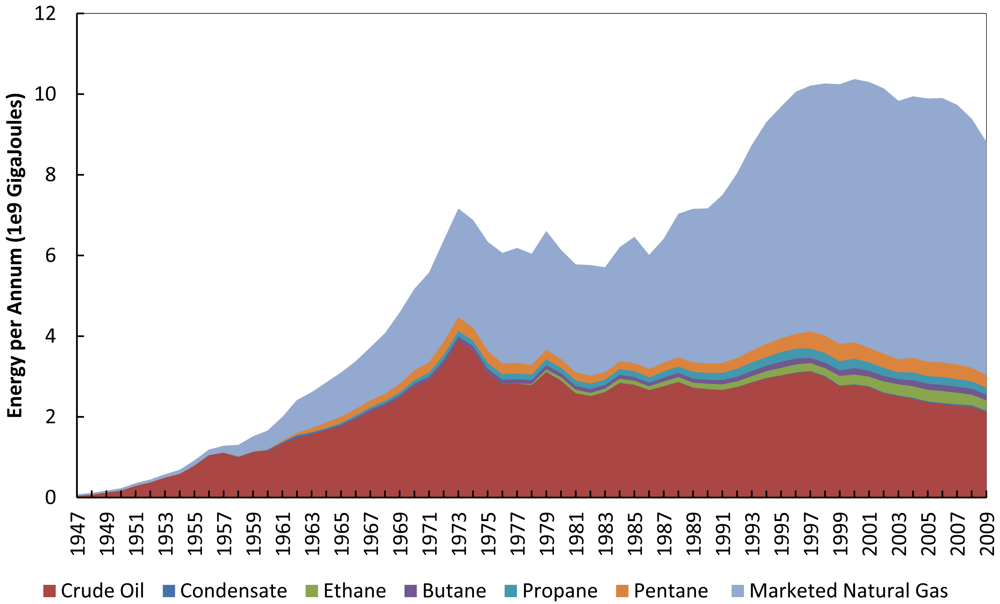
Records of petroleum production are also maintained by CAPP and published in the annual statistical handbook [22]. Summed were the values for Western Canadian conventional oil, marketed natural gas, condensates, ethane, butane, propane, and pentane plus. This paper focuses on conventional production and excludes synthetic oil from tar sands and bitumen production. States included in Western Canada are Alberta, British Columbia, Manitoba, Saskatchewan, and the Northwest Territories. 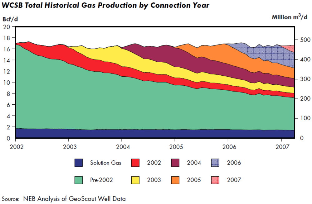The resulting energy production values are displayed in Figure 3.

3.6. Energy Input: Oil and Gas Expenditure Statistics

CAPP also maintains expenditure statistics for the petroleum industry back to 1947 [22]. Statistics are organized by state and major category. Money paid for land acquisition and royalties were excluded as these do not involve energy expenditure (money paid for land and royalties shifts to who gets to spend the industry profits, not how much energy is expended in extracting the resources). Investment categories include these Exploration expenses: Geological and Geophysical, Drilling and Other. Development expenses include: Drilling, Field Equipment, Enhanced Recovery (EOR), Gas Plants, and Other. Operating expenses include: Well and flow lines, Gas Plants and Other. All expenditures from all categories and states were summed into one value for each year.

3.7. Inflation Adjustment & Exchange Rate

The Canadian dollar expenditure statistics are nominal must be inflation corrected to the year 2002 to use the energy intensity factor calculated via EIO-LCA analysis. The inflation adjustment is intended to remove the effect of currency devaluation. The inflation adjustment was done using the Canadian CPI [23].

The adjusted results were converted into U.S. $ using the Bank of Canada Annual Average of Exchange rates for 2002 of $1.0 (U.S.) to $1.57 (Canadian) [24] and then converted into Joules of energy input using the expenditures energy intensity factor of 24 MJ/(U.S. 2002).

3.8. Combined Oil and Gas Results and Example

The results are displayed in Table 1 located in Section 2.1. A worked example for the year 2002 has an invested energy of 361 e⁶ GJ = $15 e⁹ × 24 MJ/($U.S. 2002). Net energy is 9.78 e⁹ GJ = 10.14 e⁹ GJ − 0.361 e⁹ GJ (note the scale change of 361). EROI is 28 = 10.14 e⁹ GJ / 0.361 e⁹ GJ.

3.9. Method Two: Net Energy and EROI of Western Canadian Natural Gas Wells

The method of calculating the EROI and net energy of natural gas wells is very similar to that used for oil and gas combined. Production and expenditure data were taken from the CAPP statistics and converted to units of energy. Oil production and expenditures were removed (as detailed below). The same energy intensity factor, inflation correction, and exchange rate were used as during the petroleum EROI calculation. The same EROI boundary was used, which includes the gas plants, but not refining or transportation.

3.10. Natural Gas Production Statistics

The energy from oil production was excluded, but natural gas also produced as a byproduct of oil production was included. Natural gas is trapped in solution in the liquid oil. The gas comes out of solution when the pressure drops as the oil is produced. Oil also contains some of the lighter fraction hydrocarbons, such as condensates, propane etc. The CAPP statistical handbook does not make the distinction between solution gas and non-associated gas. However, the Canadian National Energy Board provided solution gas data from private sources for the years 2000 to 2008 [13]. Solution gas accounts for about 10% of the total marketed natural gas so it is important it be removed.

For 2000 to 2008 the NEB values were used directly. To extend the solution gas estimates for the whole period of 1993 to 2009, a regression was fit between conventional oil production and the amount of solution gas for the 8 years of data. The linear correlation was high, R = 0.93 and the resulting regression was used to predict the amount of solution gas from conventional oil production for the remaining years.

The energy in the lighter hydrocarbons (natural gas liquids) needed to be apportioned between oil and gas wells as they are roughly equal to 16% of the energy in the produced natural gas (so about 1.6% of natural gas well gross energy). No public data could be found that suggested a proper ratio, so for this study it was assumed that the ratio of lighter hydrocarbons associated with oil would be the same as the ratio of natural gas associated with the oil. The solution gas ratio was used for each year and that portion of the total NGLs was removed from the gross energy produced.

3.11. Natural Gas Exploration and Development Expenditures

The CAPP expenditure statistics encompass both oil and gas expenditures, so some secondary statistic is needed to estimate how the combined expenditures should be apportioned. The statistics do separate the meters of exploration and development drilling that target oil vs. gas wells. For this study it was assumed that the apportionment of expenditure dollars would be directly related to the meters of drilling. This assumption is true only if the oil and gas wells have similar costs. As most oil and gas are produced from the same basin, this was assumed to be a reasonable apportionment (as opposed to if all the natural gas were on shore and the oil production was done much more expensively off shore).

The online version of the CAPP statistical handbook contains only the drilling distance statistics for the current year. Copies of data from past handbooks must be requested directly from CAPP for the years 1993 to 2010 [22].

Table 6. Meters drilled for oil and gas in Western Canada by year (10 e⁶ meters)

Year	Exploratory		Development
	Oil	Gas	Oil	Gas
1993	0.93	1.16	4.32	1.90
1994	1.04	2.22	4.09	3.12
1995	0.83	1.46	4.88	2.08
1996	0.97	1.29	6.34	2.57
1997	1.23	1.43	8.41	3.90
1998	0.87	2.14	3.10	3.18
1999	0.63	2.37	3.33	4.70
2000	0.79	3.19	6.06	5.92
2001	0.81	3.57	5.23	6.90
2002	0.71	2.63	4.65	6.02
2003	0.71	2.84	5.29	8.65
2004	0.79	3.96	4.91	10.84
2005	1.07	4.88	6.51	12.63
2006	1.66	4.28	6.81	11.17
2007	1.05	1.93	5.97	8.26
2008	1.44	1.41	6.05	7.84
2009	0.64	0.87	4.37	4.25

relates these hard to acquire numbers.

As an example, in 2002 the total meters drilled for oil was 0.71 e⁶ + 4.65 e⁶ = 5.36 e⁶ meters and the total meters drilled for natural gas was 2.63 e⁶ + 6.02 e⁶ = 8.65 e⁶. Natural gas was thus 61.7% of total drilling and so 61.7% of exploration and development expenditures would be apportioned to natural gas wells for 2002.

Exactly like the combined oil and gas method, royalties and land expenditures were removed.

3.12. Natural Gas Overhead Expenditures

The oil and gas well lease and gas plant overhead expenditure statistics are also intermingled. To apportion these amounts, it was assumed that expense is directly related to energy produced following a NEB technique for estimating the cost per GJ of energy produced in Western Canada [9]. The overhead expenditure amounts were split by percentage of gas-related energy production vs. oil-related energy production. For example, in 2002 10.14 e⁹ GJ of oil & natural gas was produced and 6.79 e⁹ came from natural gas wells only. Natural gas was thus 66.9% of GJ delivered and thus 66.9% of overhead expenditures were apportioned to natural gas.

3.13. Natural Gas Well Results and Example

The net energy and EROI results are shown in Table 2 of Section 2.2. The energy invested for the year 2002 was 270 e⁶ GJ = $11.25 e⁹ × 24 MJ/$. The net energy was 6.52 e⁹ GJ = 6.79 e⁹ GJ − 0.270 e⁹ GJ (note scale change of 270). The EROI 25 = 6.79 e⁹ GJ / 0.270 e⁹ GJ.

3.14. Method Three: EROI of Western Canadian Natural Gas Using Estimated Ultimate Recovery

The goal of this method was the match each year's drilling expenditures with the estimated amount of gas that would eventually be produced from that same year's wells. The Canadian National Energy Board (NEB) calculates an estimate of the amount of natural gas that will be produced by each year's wells, as described below. This estimate was used instead of the CAPP statistical handbook. The energy input was again calculated from the year's expenses, but with a slightly different apportionment between oil and gas wells.

3.15. NEB Estimated Ultimate Recovery

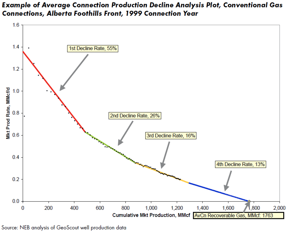
The NEB estimates the amount of natural gas that will be produced from each year's wells as part of their efforts to forecast production. They do this by collecting historical well production data and then fitting a decline curve to each well to predict when each well's production rate will decline to zero and the amount of natural gas produced at that point. Figure 9 is an example of such a curve, taken from [9], which contains a full description of the NEB methodology. The vertical axis is the rate of gas flow and the horizontal axis is total gas produced. The decline curves are calculated from prior year's well performance for the same region.

The EUR for all the wells drilled in all regions is totaled for each year. The NEB also estimates the natural gas liquids (NGL) produced. The NEB converts production volume to energy. The resulting value is reported as the estimated energy recovery and is the value this method uses for energy output. The NEB staff kindly provided updated values through 2008.

3.16. NEB Natural Gas Drilling Expenditures

The NEB provide their own estimate of natural gas well exploration and development (E&D) costs based on the CAPP statistics (which mix oil and gas production) but they use a different secondary statistic to apportion the expense dollars. Instead of the total meters of natural gas vs. oil wells drilled that this paper used in method two, the NEB used private data to add up the total number of days that drilling rigs spent drilling wells targeting natural gas (gas-intent drill days) vs. the days the drilling rigs spent drilling oil wells. The ratio of gas intent drill days vs. oil intent drill days was used to apportion the E&D expenses. The NEB method was followed here, except the NEB estimated E&D cost contains land acquisition and royalty costs that were excluded in prior methods. Removing these costs required comparing the NEB results to the original CAPP statistics and recreating the gas vs. oil ratio. The land and royalties were removed and the ratio reapplied. This allows a more direct comparison of results.

Each year's recalculated E&D cost was divided by the same year's EUR to give a resulting E&D cost per GJ of energy.

3.17. NEB Natural Gas Operating Expenditures

The operating cost was determined by summing all oil and gas production converted to heat energy and dividing by the total operating cost to determine an operating cost per GJ of energy produced. This is the same as method two for natural gas only.

3.18. Natural Gas EUR Net Energy and EROI

The costs were inflation adjusted and converted to U.S. dollars as in the prior methods. The results are reported in Tables 3 and 4 of Section 2.3. For the year 2002 the exploration and development cost was $1.19 / GJ = $6.68 e⁹ / 5.63 e⁹ GJ. The operating expense was $0.56 / GJ = $8.75 e⁹ / 10.02 e⁹ GJ.

The E&D cost per GJ and the operating cost per GJ were summed. The resulting total expenditure was converted to energy using the 24MJ/$(U.S. 2002) energy intensity value. This resulted in a ratio of Energy Input/Energy Output which is the inverse of EROI. The results were inverted to provide EROI. EROI and net energy are reported in Table 4 of Section 2.3. As an example, for 2002, the total cost was $1.74 / GJ = $1.19 + $0.56. The energy invested was 42 MJ / GJ = $1.74 / GJ × 24 MJ/$. The EROI of 24 = 1 GJ / 0.042 GJ (note the scale change of 42). And the net energy is 5.39 e⁹ GJ = 5.63 e⁹ − (0.042 × 5.63 e⁹ GJ).

4. Conclusions

This study has calculated the EROI and net energy of the Western Canadian petroleum and natural gas production by a variety of methods and the results suggest several conclusions.

4.1. The Current State of Western Canadian Natural Gas and Oil Production

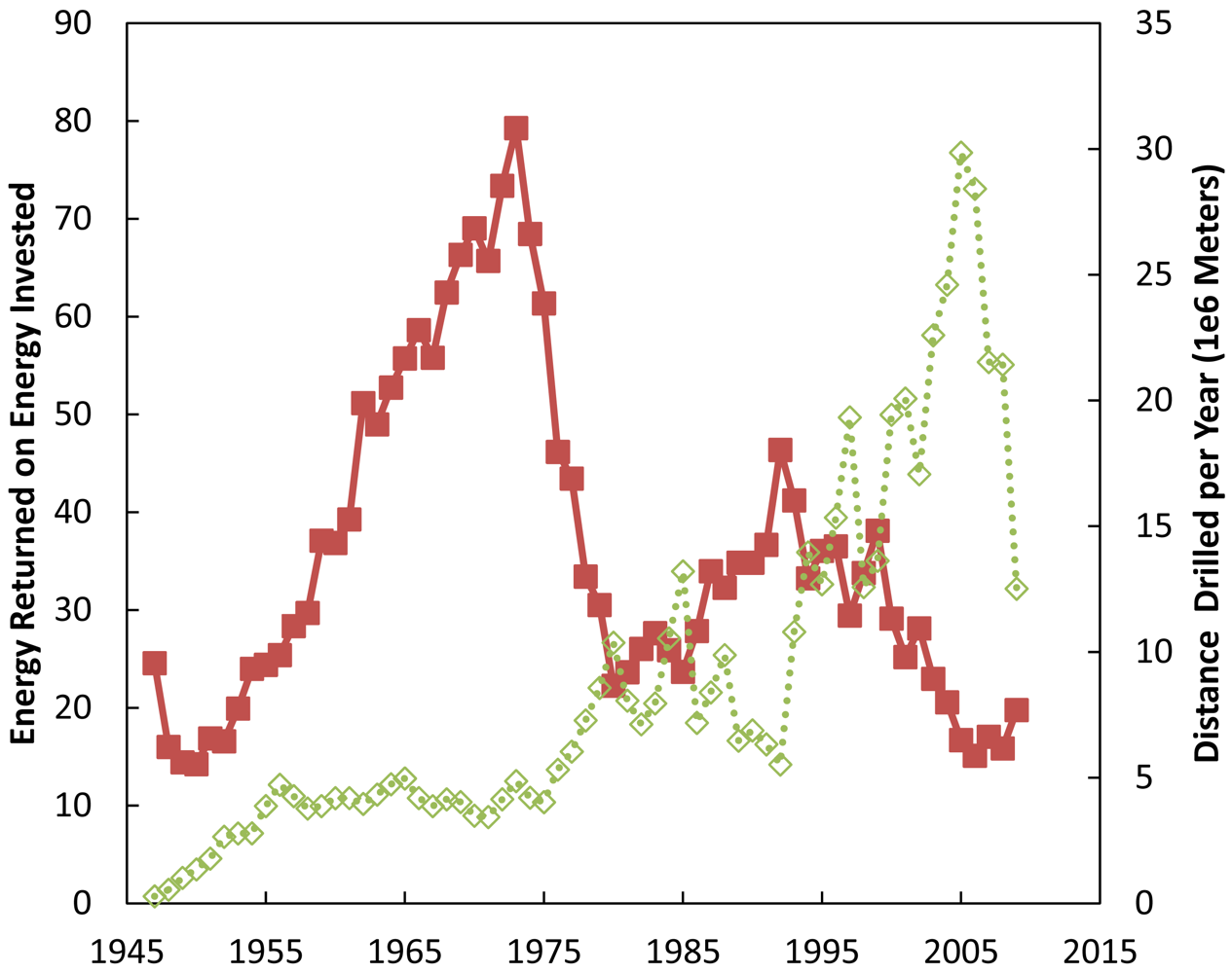
All of three methods show a downward trend in EROI during the last decade (Figure 10) and the combined oil and gas industry has fallen from a long term high EROI of 79:1 (about 1% energy consumed) to a low of 15:1 (7% energy consumed) (Figure 5).

Natural gas EROI reached an even deeper low of 14:1 (7%) or even 13:1 (8%) with the NEB EUR method. It is clear that state of the art conventional oil & natural gas extraction is unable to improve drilling efficiency as fast as depletion is reducing well quality. The fact that EROI does not rebound to match prior drilling rates and the EUR result shows no rebound indicates that well quality continues to decline. The small rebound in EROI is an result of the rolling average technique of methods one and two.

The conventional oil and gas in the WCSB has peaked. Falling well quality will likely continue to push cost up or production down. The economies that depend on this region now find themselves in the situation illustrated by Figure 1 column B, where their net energy has contracted and they will need to take action to find alternate energy supplies or improve efficiency of use.

4.2. The Net Energy Dynamics of Peak Production

The overall pattern shows a rising EROI during the early stages of exploitation followed by a peak in EROI and then declining production (Figure 5). This pattern shows the falsehood of the idea that additional investment always results in increased production. During the initial rising EROI phase, flat or falling drilling rates can increase production, and during the falling EROI phase, production can fall despite dramatic increases in investment.

There appears to be a maximum energy investment that can be sustained, which is about 15:1 to 22:1 EROI or 5% to 7% of gross energy. This might indicate a minimum EROI that can be supported while the economy grows. The minimum was higher for the oil peak than the natural gas peak and this might have been caused by inexpensive imported oil or because the economy had become more energy efficient (Figure 1 column C) allowing a lower minimum EROI.

The natural gas and oil peaks differed when analyzed using net energy. The oil peak had a peak in gross and net energy on the same year, suggesting that some outside factor was responsible for reducing investment. Natural gas showed a net energy peak before a gross production peak. This suggests that price was not the limiting factor in reducing drilling effort. Instead, from 1996 to 2005, the drilling rate for natural gas quadrupled and expenditures rose even faster, despite falling net energy and this in turn suggests that it was falling net energy was the eventual cause of economic contraction and falling prices.

A peak in net energy may be the best definition of “peak” production. When net energy peaks before gross energy it indicates that price was not the limiting factor in the effort to liberate energy. This is a likely model of world net energy production where less expensive imported energy sources cannot replace existing but declining energy sources.

A rise in EROI appears to be possible only when a new resource or region is being exploited, such as the transition from oil to gas as the primary energy production in the WCSB during the late 1980s. This study has focused on conventional natural gas production and it is very uncertain how exploitation of shale gas reserves will change the energy return.

4.3. Wider Implications

Some wider conclusions about renewable energy are suggested by this net energy study. If there is a maximum level of investment between 5% and 7% of gross energy, then economic growth may not be possible if more energy is diverted into the energy producing sector. If this minimum exists then it places a lower bound EROI on any energy source that is expected to become a major component of societies' future energy mix. For instance, nuclear power with its low EROI is likely below this level [25,26].

Also, if the maximum level of investment is 7% of output energy consumed and a renewable energy source has an EROI of 20:1, or 5%, then the 2% remaining is the maximum that may be invested into growth of the energy source without causing the economy to decline. This radically reduces the rate at which society may change the energy mix that supports it [27].

This study does not attempt to estimate the EROI or net energy of shale gas, but some caution is warranted by comparison between these results and some cursory findings for the cost of shale gas. The International Energy Agency's World Energy Outlook 2009 contained a graph showing the cost of natural gas production in the Barnett Shale (Figure 11). The core (best) counties, Johnson and Tarrant, show the lowest cost while counties outside the core production region show higher costs.

A very rough comparison can be made to the costs in this report. If the royalty amounts are subtracted and inflation adjusted into $2002 values, the Johnson County cost would be $2.94 resulting in an EROI of roughly 15:1 (7% of output consumed). This is not much higher than the lowest EROI values found in the WCSB. All the remaining Barnett Shale costs are much higher. Hill and Hood would have an EROI of 8:1 and Jack and Erath would have an EROI of roughly 5:1 (22% of output energy consumed in extraction). Given the history of the WCSB production peaks, it is hard to see how shale gas production could be much increased with such low net energy values. Shale gas may have a very short lived EROI increase over conventional while the core counties are exploited and then suffer a production collapse as EROI falls rapidly. This would fit the pattern seen with oil and then with natural gas in the WCSB.

The IEA WEO 2009 also contains Figure 12, an illustration of a world view that increasing cost will liberate more and more energy for use by society.

Conventional gas reservoirs, now peaked in production and shrinking in the WCSB, are seen as the small tip of a huge number of other resources that could be liberated with increasing investment. But falling net energy may prove this view false. If the energy return is too low, production growth may be limited or impossible from many of these energy sources. Much of the energy produced may need to be consumed during extraction. The proper shape of this diagram is likely to be a diamond with non-conventional resources forming a smaller part of the diamond underneath as denoted by the added dotted lines.