Comparing Carbon and Water Footprints for Beef Cattle Production in Southern Australia


Abstract
: Stand-alone environmental indicators based on life cycle assessment (LCA), such as the carbon footprint and water footprint, are becoming increasingly popular as a means of directing sustainable production and consumption. However, individually, these metrics violate the principle of LCA known as comprehensiveness and do not necessarily provide an indication of overall environmental impact. In this study, the carbon footprints for six diverse beef cattle production systems in southern Australia were calculated and found to range from 10.1 to 12.7 kg CO2e kg−1 live weight (cradle to farm gate). This compared to water footprints, which ranged from 3.3 to 221 L H2Oe kg−1 live weight. For these systems, the life cycle impacts of greenhouse gas (GHG) emissions and water use were subsequently modelled using endpoint indicators and aggregated to enable comparison. In all cases, impacts from GHG emissions were most important, representing 93 to 99% of the combined scores. As such, the industry's existing priority of GHG emissions reduction is affirmed. In an attempt to balance the demands of comprehensiveness and simplicity, to achieve reliable public reporting of the environmental impacts of a large number of products across the economy, a multi-indicator approach based on combined midpoint and endpoint life cycle impact assessment modelling is proposed. For agri-food products, impacts from land use should also be included as tradeoffs between GHG emissions, water use and land use are common.1. Introduction
Climate change is an issue of global significance and is potentially the defining issue of the current era [1,2]. In response, at multiple levels, governments, businesses and individuals are taking action to limit greenhouse gas (GHG) emissions. These actions are being guided by the practice of carbon footprinting [3], which when applied at the product level expresses the life cycle impact category indicator result for global warming in the units of carbon dioxide equivalents (CO2e). It has become increasingly common for businesses and industrial sector groups to use carbon footprint assessment to set priorities for GHG emissions reduction initiatives [4]. Product carbon footprints are also beginning to be reported publicly and this includes product labeling in some jurisdictions.
Although carbon footprinting has broad appeal [5], with the result being a simple and intuitively meaningful environmental indicator, concern has been raised that the practice violates the core principle of comprehensiveness in Life Cycle Assessment (LCA) [6]. What this means is that in LCA there should be consideration given to all relevant environmental impacts, to enable potential tradeoffs to be identified and assessed, and to avoid perverse outcomes from narrowly-focused actions intended to reduce environmental burden (ISO 14040: 2006). Finkbeiner [6] cites the well established environmental practices of waste water treatment and paper recycling as examples of activities which generally increase GHG emissions and if evaluated on the basis of carbon footprint alone would not be considered beneficial. Consequently, it is important to highlight that carbon footprints do not necessarily provide an indication of overall environmental impact.
One of the reasons for the growth in the uptake of the carbon footprint as a stand-alone environmental indicator is the relative ease and reasonable cost associated with conducting the assessment compared to undertaking an LCA covering all relevant impact categories [5]. For many product systems, fuel and electricity use are the key determinants of the carbon footprint and these are usually well documented within a business and supply chain. However, the problem of comprehensiveness cannot be ignored. For example, in the agriculture and food sectors, freshwater use is also recognized as a potential source of serious environmental harm [7]. Alongside climate change, global water stress is now an international issue that threatens irreversible environmental change and harmful impacts on human wellbeing [8,9]. The agriculture and food sectors are highlighted because they account for around 70% of global freshwater withdrawals [10] and are a major source of emissions responsible for freshwater quality degradation. This has led to the emergence of product water footprints as another stand-alone LCA-based environmental indicator [11], used especially in relation to food products [12-19], bio-fuels [20-22] and other water-intensive industry sectors such as electricity generation [23].
Being a streamlined LCA-based indicator, aligned with a key global environmental issue, and having less onerous inventory requirements than an LCA covering all relevant impact categories, water footprints are likely to become part of the mainstream dialogue about sustainability, much like the carbon footprint. This is being facilitated by the development of an international standard for water footprint by the International Organization for Standardization (ISO 14046). This standard will provide consistency in calculation methods and therefore comparability of results. However, in common with a carbon footprint, a water footprint is a stand-alone indicator and is therefore not an indicator of overall environmental impact, which raises again the problem of comprehensiveness discussed earlier. For many products, especially those in the agriculture and food sectors, concurrent assessment of carbon and water footprints is both realistic and desirable in order to provide a broader assessment of environmental sustainability than either a carbon or water footprint alone.
In earlier work we calculated the water footprint for six geographically-defined beef cattle production systems in southern Australia [16] using the Water Stress Index of Pfister et al. [24] following the LCA-based water footprint method of Ridoutt and Pfister [18]. With water footprinting, geographical definition of water use is critical because of the variation in local water stress and therefore variation in the environmental impacts of water use. It was found that the water footprint varied substantially, from 3.3 to 221 L H2Oe (equivalent; [18]) per kg live weight at farm gate [16]. These results can be compared to other published results; for example, fresh milk produced in a low water stress region of Victoria, Australia (1.9 L H2Oe L−1 milk at farm gate; [15]), wheat, barley and oats grown in New South Wales, Australia (0.9 to 152 L H2Oe kg−1 grain at farm gate; [19]) and fresh tomatoes grown for the Sydney market (3 to 35 L H2Oe kg−1 at farm gate; [12]). The major factors contributing to the water footprints of each beef cattle production system were also identified. In some cases, pasture irrigation was the major determinant, in others it was the operation of stock dams for livestock watering, and for another it was feedlot finishing. Such information can be used to develop strategies aimed at specifically reducing the water footprint. However, this kind of information does not assist in setting priorities for water footprint reduction relative to other environmental objectives, such as GHG emissions reduction, which is a long established priority in the livestock sector in Australia [25,26] and elsewhere [27]. In addition, a water footprint alone does not enable potential tradeoffs between carbon and water footprints to be objectively assessed.
In this current paper we address this second set of questions concerning the relationship between the carbon and water footprints of beef cattle raised in the aforementioned southern Australian production systems. To our knowledge, this is the first study of its kind, quantitatively comparing stand-alone carbon and water footprint metrics using LCA modelling. Our purpose is to provide strategic insights into the beef cattle industry in southern Australia relevant to priority setting for ongoing environmental improvement. In addition, we view this case study as a potential model of combined multi-indicator environmental assessment relevant to the agriculture and food industries more broadly.
2. Methods and Data
2.1. System Description
In Australia, the beef cattle industry operates throughout most parts of this large country. In the north (Queensland, Northern Territory and northern pastoral regions of Western Australia) cattle belonging mainly to the Bos indicus group of breeds are raised predominantly in extensive pastoral systems where individual enterprises typically exceed 100,000 ha. In contrast, in the south, Bos taurus breeds are generally raised in much smaller mixed (i.e., livestock and cropping) farming systems on native and improved pasture where a higher level of management is possible. In both the north and the south, some of these cattle are finished in feedlots, typically for between 30 to 90 days, mainly in order to achieve specific market requirements. This study concerns six geographically-defined beef cattle production systems in the Australian state of New South Wales (NSW) which is the largest region of beef cattle production in the south (5.9 million head; [28]). The six systems (Table 1) were selected in order to be diverse in farm practice (pasture and feedlot finishing), product (yearling to heavy steers), environment (high-rainfall coastal and semi-arid inland) and local water stress. Further details about these systems, including the life cycle inventory data sources and modeling, are described in Ridoutt et al. [16].
2.2. Carbon Footprint Modeling
The overall approach to modeling the carbon footprint followed PAS 2050, the widely adopted process LCA-based method of calculating the GHG emission of a product [29]. The functional unit was one kg live weight (LW) of beef cattle destined for slaughter at farm gate. This functional unit enabled comparison of livestock of varying size and age at the point of marketing. The calculation of GHG emissions from livestock enteric fermentation, manure and urine followed the country specific, IPCC Tier 2 approach used in Australia's national GHG inventory [30], taking into account herd structure (on a daily time step; [16]), feed quality and growth rate. Emissions from agricultural soils as a result of inorganic nitrogen fertiliser application and the residue of cultivated leguminous pastures were also calculated following the method of the Australian national GHG inventory [30]. Land use change (deforestation) did not feature in any of the systems and possible changes in soil carbon were ignored due to a lack of relevant data. The Australasian Unit Process Life Cycle Inventory [31], Australian environmental input-output data [32] and various CSIRO internal sources provided data on GHG emissions associated with fuels, fertilizers, supplementary feeds (grain and pasture hay), veterinary and marketing services used in farming, fuels used to transport livestock between farms and to feedlots (where relevant), fuels used to deliver feed components to feedlots, and fuels, electricity and feed components consumed in feedlots. To calculate the carbon footprint the latest 100-year global warming potentials for GHGs published by the IPCC were used [33].
2.3. Life Cycle Impact Assessment Endpoint Modeling
Damages to human health (Disability Adjusted Life Years, DALY) and ecosystem health (loss of species diversity, species·m2·yr) due to GHG emissions were modeled using characterization factors reported by de Schryver et al. [34], taking the Hierarchist cultural perspective. The Hierarchist cultural perspective was chosen as the time horizon of 100 years corresponds with PAS 2050 [29] and draft ISO 14067, and because it presents a less extreme combination of value choices compared to the Individualist and Egalitarian perspectives. The Hierarchist cultural perspective is also used by Pfister et al. [24], in the method adopted in this study to assess damages to human health, ecosystem health and depletion of resources (MJ) due to consumptive water use. This method of Pfister et al. [24] was chosen to assess water use impacts because it was the only method enabling a comprehensive impact assessment of freshwater consumption on the endpoint level [11] that was operationalized for use in an established life cycle impact assessment methodology. Using normalization factors and weights for the Hierarchist perspective taken from the Eco-indicator 99 life cycle impact assessment methodology ([35] p. 113], aggregated scores were calculated (points kg−1 LW). Damages arising from GHG emissions and water use were then compared.
3. Results and Discussion
3.1. Carbon Footprint of Beef Cattle
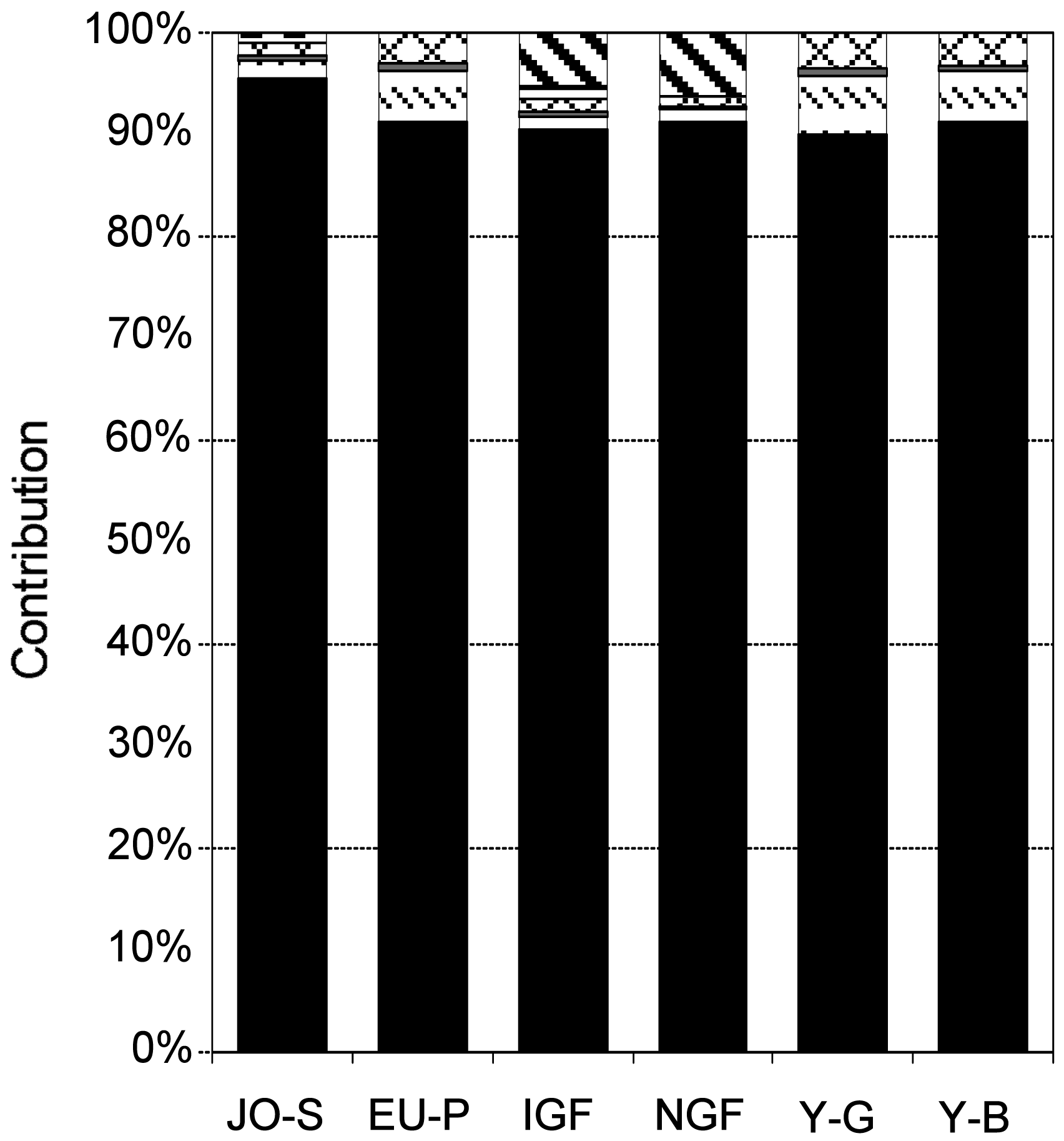
For the six southern Australian beef cattle production systems assessed, the carbon footprint (cradle to farm gate) ranged from 10.1 to 12.7 kg CO2e kg−1 LW (Table 2). In all cases, the carbon footprint was overwhelmingly influenced by methane emissions (87 to 92%; Figure 1), predominantly related to the livestock themselves (Figure 2), although the livestock emissions also included nitrous oxide emissions from dung and urine in addition to enteric methane and methane from dung. These results fall within the range of reported estimates for beef cattle GHG emissions, which typically range from about 6 to 20 kg CO2e kg−1 LW [36-43]. In other extensive pastoral systems with lower productivity, the carbon footprint of beef cattle can exceed this range, and become extremely large where substantial deforestation occurs and this is included in the carbon footprint calculation (e.g., >350 kg CO2e kg−1 LW; [44]).
For the six beef cattle production systems described in this paper, the differences in carbon footprint between the systems were relatively small and not obviously correlated with any particular variable. For example, cattle produced in the two systems which included feedlot finishing had both the lowest and the highest carbon footprints (Table 2). In general, feedlot finished livestock are expected to have a lower carbon footprint [43,45] due to the more nutritious feedlot diet reducing the time for animals to achieve their target weight and therefore the life cycle ruminant methane emissions. One point of difference between the systems was the average age at which cows gave birth to their first calf, which was 36 months in the system with the highest carbon footprint compared to 24 months for the others [16]. Hence the importance of reproduction rate in the overall carbon footprint of beef cattle.
3.2. Comparison of Impacts from GHG Emissions and Water Use
In every case, for the six southern Australian beef cattle production systems, the potential environmental impacts from GHG emissions greatly exceeded the potential impacts from consumptive water use, representing 93 to 99% of the combined Eco-indicator 99 scores (Table 3). Despite there being a relatively large range in water footprint, from 3.3 to 221 L H2Oe kg−1 LW (Table 2), the contribution of water use to the combined environmental impact scores was always small. As such, for beef production systems of the kind represented by these case studies, our results support an ongoing emphasis on GHG emissions reduction. Warnings about the impacts of water use in relation to livestock production [46-51] may be relevant in some particular cases, but are not generally relevant in southern Australia.
Herein lies the danger of stand-alone environmental indicators which report on a single environmental impact. If taken alone and not put in the context of other potential environmental impacts, they could misdirect resources away from actions which are more important. The evidence we present supports a continuing emphasis on carbon footprint reduction not a diversion of resources to lower water footprints for the types of beef cattle production systems broadly represented by the case studies. Our results show that warnings about the water footprint of livestock have the potential to motivate misdirection of environmental improvement efforts and such warnings need to be substantiated by science-based evidence relevant to the particular livestock production system and environment in question.
Another concern about stand-alone indicators is the issue of tradeoffs. Of course, an intervention that led to a concurrent reduction in both carbon and water footprint would be highly desirable. However, tradeoffs between greenhouse gas emissions and water use are not uncommon. For example, to reduce livestock enteric methane emissions one very viable strategy is to improve forage quality [26], which can often be achieved through greater use of pasture irrigation and fertilization, actions which have the potential to raise water footprints. That said, for the six production systems assessed in this study it would appear that strategies which reduced the carbon footprint, but which also led to a moderate increase in water footprint, would result in an overall reduction in combined environmental burden.
3.3. Streamlined Multi-Indicator Assessment of Agri-Food Products
This study has been based on a combination of midpoint and endpoint life cycle impact assessment indicators in order to take advantage of the benefits of each. Midpoint indicators are the result of modelling that extends only part way along the cause-effect chain [52]. For example, carbon footprinting models the global warming potential of GHG emissions, expressed in the units CO2e. In this example, global warming is a midpoint in the environmental mechanism whereby temperature increases ultimately impact on human health (malnutrition, diarrhoea, malaria, heat stress, etc.; [34]), and ecosystems (species disappearance). Likewise, the water footprints calculated in this study are a midpoint indicator, describing impacts on water stress [18], which ultimately lead to impacts on human health, ecosystems and environmental resource depletion [24]. Compared to endpoint indicators, midpoint indicators are generally regarded as having greater reliability (i.e., lower model and parameter uncertainty), higher transparency (i.e., based on less complex models with fewer assumptions and value choices and which are more readily explained), and as being more suitable for communication to stakeholders (i.e., having greater intuitive meaning as well as more recognizable and acceptable units) [52]. On the other hand, endpoint indicators are generally regarded as having greater relevance. It is the damages to human health, ecosystems and depletion of resources which is the ultimate environmental concern. In addition, endpoint indicators are often preferred where aggregation of results is desired, such as in this study where damages arising from GHG emissions and water use were aggregated and compared. Weighting factors exist at the endpoint level (e.g., Eco-indicator 99) which have been applied in a consistent way in many LCA studies across the world. In contrast, there are no recognised or commonly adopted weighting factors for GHG emissions and water use at the midpoint level.
Without question, the most informed environmental decision making will occur when all relevant environmental impacts are considered in an LCA. However, the effort and expense of completing such a task means that an LCA tends to be performed selectively in strategically important decision making contexts and the likelihood of process-based LCA being applied to a great many individual products in the economy is perhaps small [53]. In addition, the results of an LCA are rich in detail, but difficult to convey to a remote and non-technical audience (e.g., a product environmental label or declaration). The other extreme is a single stand-alone indictor, like a carbon footprint, which may achieve widespread community awareness, but as mentioned in the Introduction, will violate the principle of comprehensiveness and potentially promote poor decision making in terms of overall environmental impact. The solution, it seems, lies between these two extremes, in a small set of streamlined sustainability indicators which are chosen because of their high environmental relevance for the product category of interest, combined with an aggregated score. We have demonstrated this general approach in this study using carbon and water footprints as an example.
For agri-food products, impacts from GHG emissions, water use and land use are thought to be the highest concern. However, there are also many tradeoffs between these. For example, land can be used for biodiversity conservation and carbon sequestration or it can be used for food production, and some forms of agriculture support more biodiversity than others. In regard to water and land, a small quantity of irrigated land can produce the same quantity of food as a larger area of non-irrigated land. These tradeoffs underscore the futility of comparing the merits of one food production system or product over another using a single stand-alone indicator. At this point in time, impact assessment methods for land use in LCA are under development, supported by a project group working under the auspices of the United Nations Environment Programme and the Society of Environmental Toxicology and Chemistry (UNEP-SETAC) Life Cycle Initiative [54]. The challenge is that the impacts of land use depend not only on the quantity of land used, but also its quality and the intensity of production. Modelling the environmental impacts of land use is therefore not straightforward. Nevertheless, the future direction of our research is to integrate land use impacts with carbon and water footprints in the manner demonstrated in this paper. For agri-food products, these three indicators probably represent an appropriate balance between comprehensiveness and practicality.
4. Conclusions
This study has shown, for a range of beef cattle production systems in NSW, Australia, that the environmental impacts from GHG emissions far exceed the environmental impacts from water use. As such, the industry's current priority of GHG emissions reduction is confirmed. Furthermore, for beef cattle production systems of the type represented in this study, GHG emissions reduction that was achieved at the expense of a moderate increase in water use, would likely lead to an overall improved environmental outcome. Using the methods demonstrated in this report, particular scenarios involving GHG emission and water use tradeoffs can now be evaluated.
In addition, in an attempt to balance the demands of comprehensiveness and practicality, a multi-indicator approach based on combined midpoint and endpoint life cycle modelling was presented. It was argued that a single stand-alone indicator, such as a carbon footprint, is not sufficient to motivate wise decision making which leads to reduced overall environmental burden. However, if quantitative environmental assessment based on life cycle assessment is to be applied to a large number of products, produced by small and large companies alike, then the costs, largely driven by inventory requirements, cannot be too onerous. In addition, if the results are to be widely disseminated throughout the economy then the results must be relevant to a non-technical audience. We believe these demands are best able to be met through the multi-indicator approach based on a selection of industry-sector relevant midpoint indicators combined with an aggregated endpoint result. In this study, such an approach based on carbon and water footprints was demonstrated. However, for agri-food products, the inclusion of impacts from land use (land use footprint) is also highly desirable.
 , nitrous oxide
 and carbon dioxide
 to the carbon footprint of beef cattle (cradle to farm gate) produced in six geographically-defined systems in southern Australia. JO-S: Japanese ox grass-fed steers (Scone); EU-P: EU cattle (Parkes); IGF: Inland weaners, grass fattened and feedlot finished (Walgett, Gunnedah, Quirindi); NGF: North coast weaners, grass fattened and feedlot finished (Casino, Glen Innes, Rangers Valley); Y-G: Yearling (Gundagai); Y-B: Yearling (Bathurst).
, nitrous oxide
and carbon dioxide
to the carbon footprint of beef cattle (cradle to farm gate) produced in six geographically-defined systems in southern Australia. JO-S: Japanese ox grass-fed steers (Scone); EU-P: EU cattle (Parkes); IGF: Inland weaners, grass fattened and feedlot finished (Walgett, Gunnedah, Quirindi); NGF: North coast weaners, grass fattened and feedlot finished (Casino, Glen Innes, Rangers Valley); Y-G: Yearling (Gundagai); Y-B: Yearling (Bathurst).
to the carbon footprint of beef cattle (cradle to farm gate) produced in six geographically-defined systems in southern Australia. JO-S: Japanese ox grass-fed steers (Scone); EU-P: EU cattle (Parkes); IGF: Inland weaners, grass fattened and feedlot finished (Walgett, Gunnedah, Quirindi); NGF: North coast weaners, grass fattened and feedlot finished (Casino, Glen Innes, Rangers Valley); Y-G: Yearling (Gundagai); Y-B: Yearling (Bathurst).
, nitrous oxide
and carbon dioxide
to the carbon footprint of beef cattle (cradle to farm gate) produced in six geographically-defined systems in southern Australia. JO-S: Japanese ox grass-fed steers (Scone); EU-P: EU cattle (Parkes); IGF: Inland weaners, grass fattened and feedlot finished (Walgett, Gunnedah, Quirindi); NGF: North coast weaners, grass fattened and feedlot finished (Casino, Glen Innes, Rangers Valley); Y-G: Yearling (Gundagai); Y-B: Yearling (Bathurst).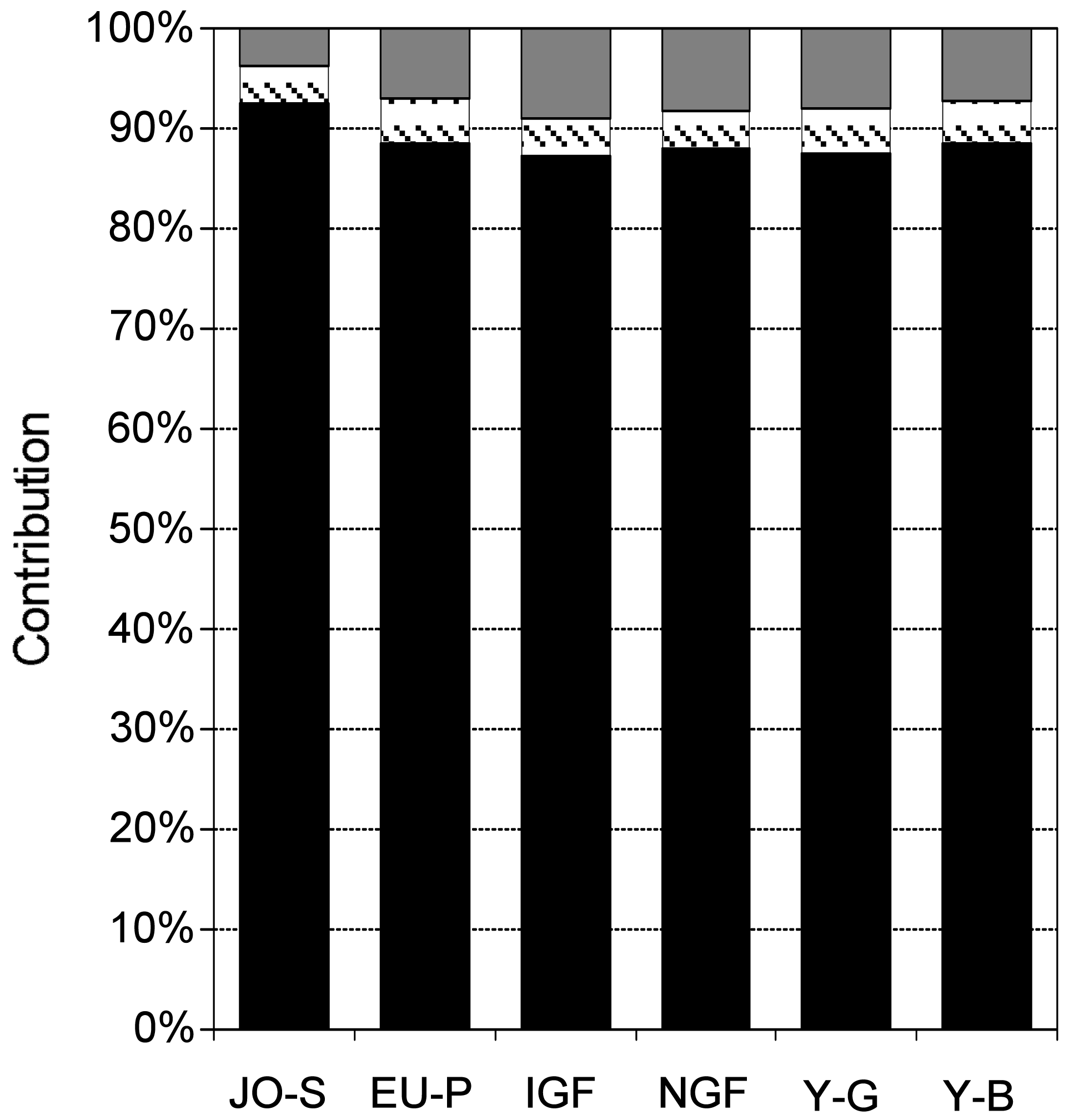 , fertilizer used on pasture
, leguminous pastures
, other farm inputs
, fertilizer used on pasture
, leguminous pastures
, other farm inputs
 , supplementary feeds used on-farm
 , livestock transport
 , and feedlot finishing
 to the carbon footprint of beef cattle (cradle to farm gate) produced in six geographically-defined systems in southern Australia. JO-S: Japanese ox grass-fed steers (Scone); EU-P: EU cattle (Parkes); IGF: Inland weaners, grass fattened and feedlot finished (Walgett, Gunnedah, Quirindi); NGF: North coast weaners, grass fattened and feedlot finished (Casino, Glen Innes, Rangers Valley); Y-G: Yearling (Gundagai); Y-B: Yearling (Bathurst).
, fertilizer used on pasture
, leguminous pastures
, other farm inputs
, supplementary feeds used on-farm
, livestock transport
, and feedlot finishing
to the carbon footprint of beef cattle (cradle to farm gate) produced in six geographically-defined systems in southern Australia. JO-S: Japanese ox grass-fed steers (Scone); EU-P: EU cattle (Parkes); IGF: Inland weaners, grass fattened and feedlot finished (Walgett, Gunnedah, Quirindi); NGF: North coast weaners, grass fattened and feedlot finished (Casino, Glen Innes, Rangers Valley); Y-G: Yearling (Gundagai); Y-B: Yearling (Bathurst).
to the carbon footprint of beef cattle (cradle to farm gate) produced in six geographically-defined systems in southern Australia. JO-S: Japanese ox grass-fed steers (Scone); EU-P: EU cattle (Parkes); IGF: Inland weaners, grass fattened and feedlot finished (Walgett, Gunnedah, Quirindi); NGF: North coast weaners, grass fattened and feedlot finished (Casino, Glen Innes, Rangers Valley); Y-G: Yearling (Gundagai); Y-B: Yearling (Bathurst).
, fertilizer used on pasture
, leguminous pastures
, other farm inputs
, supplementary feeds used on-farm
, livestock transport
, and feedlot finishing
to the carbon footprint of beef cattle (cradle to farm gate) produced in six geographically-defined systems in southern Australia. JO-S: Japanese ox grass-fed steers (Scone); EU-P: EU cattle (Parkes); IGF: Inland weaners, grass fattened and feedlot finished (Walgett, Gunnedah, Quirindi); NGF: North coast weaners, grass fattened and feedlot finished (Casino, Glen Innes, Rangers Valley); Y-G: Yearling (Gundagai); Y-B: Yearling (Bathurst).

| Production system | Main product | Location(s) | Mean max temp (°C) | Mean min temp (°C) | Mean rainfall (mm yr−1) | WSIc |
|---|---|---|---|---|---|---|
| Japanese ox— grass-fed steers | 24–36 mth old steers 340 kg DW b | Scone | 24.1 | 11.0 | 644 | 0.032 |
| EU cattle | 24–30 mth old steers 280–300 kg DW | Parkes | 23.4 | 10.9 | 584 | 0.815 |
| Inland weaners, grass fattened and feedlot finished | 24 mth old steers 585 kg LW | Walgett | 0.021 | |||
| Gunnedah | 26.9 26.0 24.6 | 12.5 10.9 8.9 | 477 619 683 | 0.021 | ||
| Quirindi | 0.021 | |||||
| North coast weaners, grass fattened and feedlot finished | 24 mth old steers 585 kg LW | Casino Glen | 0.012 | |||
| Innes Rangers | 26.7 19.4 19.4 | 13.2 7.3 7.3 | 1096 849 849 | 0.021 | ||
| Valley | 0.021 | |||||
| Yearling | 12–15 mth old yearling 185–205 kg DW | Gundagai | 22.3 | 8.5 | 713 | 0.815 |
| Yearling | 12–15 mth old yearling 185–205 kg DW | Bathurst | 19.8 | 6.8 | 635 | 0.021 |
aReproduced, with permission [16].bDW: dressed weight or dressed carcass weight after removal of hide, head, feet, tail and internal organs; LW: live weight.cWSI: water stress index [24].
| Production system (Location) | Carbon footprint | Water footprint |
|---|---|---|
| Japanese ox - grass-fed steers (Scone) | 10.2 | 14.4 |
| EU cattle (Parkes) | 10.8 | 68.3 |
| Inland weaners/ grass fattened/ feedlot finished (Walgett, Gunnedah, Quirindi) | 10.1 | 9.1 |
| North coast weaners/ grass fattened/ feedlot finished (Casino, Glen Innes, Rangers Valley) | 12.7 | 7.7 |
| Yearling (Gundagai) | 10.4 | 221 |
| Yearling (Bathurst) | 10.6 | 3.3 |
| Production system | GHG emissions | Water usea | GHG emission contribution | ||||
|---|---|---|---|---|---|---|---|
| Human health | Ecosystems | Aggregated score | Ecosystems | Resources | Aggregated score | ||
| Japanese ox— grass-fed steers | 2.10 × 10⁻⁶ | 2.19 | 2.25 × 10⁻¹ | 1.00 × 10⁻¹ | 1.12 × 10⁻³ | 0.78 × 10⁻² | 96.6 |
| EU cattle | 2.26 × 10⁻⁶ | 2.36 | 2.43 × 10⁻¹ | 0.57 × 10⁻¹ | 1.51 × 10⁻³ | 0.45 × 10⁻² | 98.2 |
| Inland weaners, grass fattened and feedlot finished | 2.11 × 10⁻⁶ | 2.19 | 2.26 × 10⁻¹ | 1.99 × 10⁻¹ | 1.77 × 10⁻³ | 1.56 × 10⁻² | 93.5 |
| North coast weaners, grass fattened and feedlot finished | 2.65 × 10⁻⁶ | 2.76 | 2.84 × 10⁻¹ | 0.96 × 10⁻¹ | 1.79 × 10⁻³ | 0.75 × 10⁻² | 97.4 |
| Yearling (Gundagai) | 2.17 × 10⁻⁶ | 2.26 | 2.33 × 10⁻¹ | 1.74 × 10⁻¹ | 1.25 × 10⁻³ | 1.36 × 10⁻² | 94.5 |
| Yearling (Bathurst) | 2.22 × 10⁻⁶ | 2.31 | 2.38 × 10⁻¹ | 0.35 × 10⁻¹ | 1.18 × 10⁻³ | 0.28 × 10⁻² | 98.9 |
aIn the Australian context, there are no damages to human health associated with water use [24].
Acknowledgments
We thank Beverley Henry (Queensland University of Technology) and Peter Carberry (CSIRO) who reviewed the manuscript and made helpful suggestions.
References and Notes
- The Century's Defining Issue. The Economist, 3 December 2009. Available online: http://www.economist.com/blogs/freeexchange/2009/12/the_centurys_defining_issue (accessed on 9 June 2011).
- Climate change ‘defining issue of our era’ says Ban Ki-moon, hailing G8 action. 2007. UN News Service Web site Available online: http://www.un.org/apps/news/printnewsAr.asp?nid=22836 (accessed on 9 June 2011).
- Peters, G.P. Carbon footprints and embodied carbon at multiple scales. Curr. Opin. Environ. Sustain. 2010, 2, 245–250. [Google Scholar]
- Wiedmann, T.O.; Lenzen, M.; Barrett, J.R. Companies on the scale: Comparing and benchmarking the sustainability performance of businesses. J. Ind. Ecol. 2009, 13, 361–383. [Google Scholar]
- Weidema, B.P.; Thrane, M.; Christensen, P.; Schmidt, J.; Løkke, S. Carbon footprint: A catalyst for life cycle assessment? J. Ind. Ecol. 2008, 12, 3–6. [Google Scholar]
- Finkbeiner, M. Carbon footprinting—Opportunities and threats. Int. J. Life Cycle Assess 2009, 14, 91–94. [Google Scholar]
- Ridoutt, B.G. Development and application of a water footprint metric for agricultural products and the food industry. In Towards Life Cycle Sustainability Management; Finkbeiner, M., Ed.; Springer: Dordrecht, The Netherlands, 2011; pp. 183–192. [Google Scholar]
- Rockström, J.; Steffen, W.; Noone, K.; Persson, Å; Chapin, F.S.; Lambin, E.F.; Lenton, T.M.; Scheffer, M.; Folke, C.; Schellnhuber, H.J.; et al. A safe operating space for humanity. Nature 2009, 461, 472–475. [Google Scholar]
- Ridoutt, B.G.; Pfister, S. Reducing humanity's water footprint. Environ. Sci. Technol 2010, 44, 6019–6021. [Google Scholar]
- The United Nations World Water Development Report 3: Water in a Changing World; The United Nations Educational, Scientific and Cultural Organization: Paris, France, 2009.
- Berger, M.; Finkbeiner, M. Water footprinting: How to address water use in life cycle assessment? Sustainability 2010, 2, 919–944. [Google Scholar]
- Page, G.; Ridoutt, B.; Bellotti, B. Fresh tomato production for the Sydney market: An evaluation of options to reduce freshwater scarcity from agricultural water use. Agric. Water Manag. 2011, 100, 18–24. [Google Scholar]
- Ridoutt, B.G.; Eady, S.J.; Sellahewa, J.; Simons, L.; Bektash, R. Water footprinting at the product brand level: Case study and future challenges. J. Clean. Prod. 2009, 17, 1228–1235. [Google Scholar]
- Ridoutt, B.G.; Juliano, P.; Sanguansri, P.; Sellahewa, J. The water footprint of food waste: Case study of fresh mango in Australia. J. Clean. Prod. 2010, 18, 1714–1721. [Google Scholar]
- Ridoutt, B.G.; Williams, S.R.O.; Baud, S.; Fraval, S.; Marks, N. The water footprint of dairy products: Case study involving skim milk powder. J. Dairy Sci. 2010, 93, 5114–5117. [Google Scholar]
- Ridoutt, B.G.; Sanguansri, P.; Freer, M.; Harper, G. Water footprint of livestock: Comparison of six geographically-defined beef production systems. Int. J. Life Cycle Assess. in press.
- Ridoutt, B.G.; Sanguansri, P.; Nolan, M.; Marks, N. Meat consumption and water scarcity: Beware of generalizations. J. Clean. Prod. in press.
- Ridoutt, B.G.; Pfister, S. A revised approach to water footprinting to make transparent the impacts of consumption and production on global freshwater scarcity. Glob. Environ. Change 2010, 20, 113–120. [Google Scholar]
- Ridoutt, B.G.; Poulton, P.L. Dryland and irrigated cropping systems: Comparing the impacts of consumptive water use. Proceedings of the 7th International Conference on Life Cycle Assessment in the Agri-Food Sector (LCA Food 2010), Bari, Italy, 22–24 September 2010; Notarnicola, B., Settanni, E., Tassielli, G., Giungato, P., Eds.; Università degli Studi di Bari Aldo Moro: Bari, Italy, 2010. [Google Scholar]
- Dominguez-Faus, R.; Powers, S.E.; Burken, J.G.; Alvarez, P.J. The water footprint of biofuels: A drink or drive issue? Environ. Sci. Technol. 2009, 43, 3005–3010. [Google Scholar]
- Jeswani, H.K.; Azapagic, A. Water footprint: Methodologies and a case study for assessing the impacts of water use. J. Clean. Prod. 2011, 19, 1288–1299. [Google Scholar]
- Scown, C.D.; Horvath, A.; McKone, T.E. Water footprint of U.S. transportation fuels. Environ. Sci. Technol. 2011, 45, 2541–2553. [Google Scholar]
- Pfister, S.; Saner, D.; Koehler, A. The environmental relevance of freshwater consumption in global power production. Int. J. Life Cycle Assess. 2011, 16, 580–591. [Google Scholar]
- Pfister, S.; Koehler, A.; Hellweg, S. Assessing the environmental impacts of freshwater consumption in LCA. Environ. Sci. Technol. 2009, 43, 4098–4104. [Google Scholar]
- Cottle, D.J.; Nolan, J.V.; Wiedermann, S.G. Ruminant enteric methane mitigation: A review. Anim. Prod. Sci. 2011, 51, 491–514. [Google Scholar]
- Eckard, R.J.; Grainger, C.; de Klein, C.A.M. Options for abatement of methane and nitrous oxide from ruminant production: A review. Livest. Sci. 2010, 130, 47–56. [Google Scholar]
- Martin, C.; Morgavi, D.P.; Doreau, M. Methane mitigation in ruminants: From microbe to the farm scale. Animal 2010, 4, 351–365. [Google Scholar]
- 7121.0 Agricultural Commodities, Australia, 2008–09; Australian Bureau of Statistics, Commonwealth of Australia: Canberra, Australia, 2010. Available online: http://abs.gov.au (accessed on 8 September 2010).
- PAS2050:2008, Specification for the Assessment of the Life Cycle Greenhouse Gas Emissions of Goods and Services; British Standards Institution: London, UK, 2008.
- Australian Methodology for the Estimation of Greenhouse Gas Emissions and Sinks 2006: Agriculture; National Greenhouse Gas Inventory Committee. Australian Government, Department of Climate Change: Canberra, Austrilia, 2007.
- Grant, T. Australasian LCA Database: Manual for SimaPro Implementation; Life Cycle Strategies: Melbourne, Austrilia, 2010. [Google Scholar]
- Foran, B.; Lenzen, M.; Dey, C. Balancing Act; CSIRO: Highett, VIC, Australia, 2005. [Google Scholar]
- Forster, P.; Ramaswamy, V. Changes in atmospheric constituents and in radiative forcing. In Contribution of Working Group I to the Fourth Assessment Report of the Intergovernmental Panel on Climate Change; Solomon, S., Qin, D., Manning, M., Chen, Z., Marquis, M., Averyt, K.B., Tignor, M., Miller, H.L., Eds.; Cambridge University Press: Cambridge, UK, 2007; pp. 129–234. [Google Scholar]
- De Schryver, A.M.; Brakkee, K.W.; Goedkoop, M.J.; Huijbregts, M.A.J. Characterization factors for global warming in life cycle assessment based on damages to humans and ecosystems. Environ. Sci. Technol. 2009, 43, 1689–1695. [Google Scholar]
- Goedkoop, M.; Spriensma, R. The Eco-indicator 99: A Damage Oriented Method for Life Cycle Assessment: Methodology Report, 2nd ed.; Pré Consultants B.V.: Amersfoort, The Netherlands, 2000. [Google Scholar]
- Beauchemin, K.A.; Janzen, H.H.; Little, S.M.; McAllister, T.A.; McGinn, S.M. Life cycle assessment of greenhouse gas emissions from beef production in western Canada: A case study. Agric. Syst. 2010, 103, 371–379. [Google Scholar]
- Casey, J.W.; Holden, N.M. Quantification of GHG emissions from sucker-beef production in Ireland. Agric. Syst. 2006, 90, 79–98. [Google Scholar]
- Crosson, P.; Shalloo, L.; O'Brien, D.; Lanigan, G.J.; Foley, P.A.; Boland, T.M.; Kenny, D.A. A review of whole farm systems models of greenhouse gas emissions from beef and dairy cattle production systems. Anim. Feed Sci. Technol. 2011, 166‐167, 29–45. [Google Scholar]
- De Vries, M.; de Boer, I.J.M. Comparing environmental impacts for livestock products: A review of life cycle assessments. Livest. Sci. 2010, 128, 1–11. [Google Scholar]
- Lesschen, J.P.; van den Berg, M.; Westhoek, H.J.; Witzke, H.P.; Oenema, O. Greenhouse gas emission profiles of European livestock sectors. Anim. Feed Sci. Technol. 2011, 166‐167, 16–28. [Google Scholar]
- Nguyen, T.L.T.; Hermansen, J.E.; Mogensen, L. Environmental consequences of different beef production systems in the EU. J. Clean. Prod. 2010, 18, 756–766. [Google Scholar]
- Pelletier, N.; Pirog, R.; Rasmussen, R. Comparative life cycle environmental impacts of three beef production strategies in the Upper Midwestern United States. Agric. Syst. 2010, 103, 380–389. [Google Scholar]
- Peters, G.M.; Rowley, H.V.; Wiedemann, S.; Tucker, R.; Short, M.D.; Schulz, M. Red meat production in Australia: Life cycle assessment and comparison with overseas studies. Environ. Sci. Technol. 2010, 44, 1327–1332. [Google Scholar]
- Cederberg, C.; Persson, U.M.; Neovius, K.; Molander, S.; Clift, R. Including carbon emissions from deforestation in the carbon footprint of Brazilian beef. Environ. Sci. Technol. 2011, 45, 1773–1779. [Google Scholar]
- Vergé, X.P.C.; Dyer, J.A.; Desjardins, R.L.; Worth, D. Greenhouse gas emissions from the Canadian beef industry. Agric. Syst. 2008, 98, 126–134. [Google Scholar]
- Liu, J.G.; Yang, H.; Savenije, H.H.G. China's move to higher-meat diet hits water security. Nature 2008, 454, 397. [Google Scholar]
- Marlow, H.J.; Hayes, W.K.; Soret, S.; Carter, R.L.; Schwab, E.R.; Sabaté, J. Diet and environment: Does what you eat matter? Am. J. Clin. Nutr. 2009, 89, 1699S–1703S. [Google Scholar]
- Mekonnen, M.M.; Hoekstra, A.Y. The Green, Blue and Grey Water Footprint of Farm Animals and Animal Products; UNESCO-IHE, Institute for Water Education: Delft, The Netherlands, 2010. [Google Scholar]
- The Environmental Food Crisis: The Environment's Role in Averting Future Food Crises; Nellemann, C., MacDevette, M., Manders, T., Eickhout, B., Svihus, B., Prins, A.G., Kaltenborn, B.P., Eds.; UNEP/GRIP-Arendal: Arendal, Norway, 2009.
- Pearce, F. Thirsty meals that suck the world dry. New Sci. 1997, 2067, 7. [Google Scholar]
- Steinfeld, H.; Gerber, P.; Wassenaar, T.; Castel, V.; Rosales, M.; de Haan, C. Livestock's Long Shadow: Environmental Issues and Options; FAO: Rome, Italy, 2006. [Google Scholar]
- Bare, J.C.; Hofstetter, P.; Pennington, D.W.; Udo de Haes, H.A. Midpoints versus endpoints: The sacrifices and benefits. Int. J. Life Cycle Assess. 2000, 5, 319–326. [Google Scholar]
- Milà i Canals, L.; Sim, S.; García-Suárez, T.; Neuer, G.; Herstein, K.; Kerr, C.; Rigarlsford, G.; King, H. Estimating the greenhouse gas footprint of Knorr. Int. J. Life Cycle Assess. 2011, 16, 50–58. [Google Scholar]
- Müller-Wenk, R.; Brandão, M. Climatic impact of land use in LCA: Carbon transfers between vegetation/soil and air. Int. J. Life Cycle Assess. 2010, 15, 172–182. [Google Scholar]
- Conflict of Interest: This study was jointly funded by Meat and Livestock Australia and CSIRO Sustainable Agriculture National Research Flagship, and one author, Gregory Harper, has been an independent, non-executive director of Meat and Livestock Australia since November 2009. That said, the authors have exercised complete freedom in designing the research and interpreting the data.
© 2011 by the authors; licensee MDPI, Basel, Switzerland. This article is an open access article distributed under the terms and conditions of the Creative Commons Attribution license (http://creativecommons.org/licenses/by/3.0/).
Share and Cite
Ridoutt, B.G.; Sanguansri, P.; Harper, G.S. Comparing Carbon and Water Footprints for Beef Cattle Production in Southern Australia. Sustainability 2011, 3, 2443-2455. https://doi.org/10.3390/su3122443
Ridoutt BG, Sanguansri P, Harper GS. Comparing Carbon and Water Footprints for Beef Cattle Production in Southern Australia. Sustainability. 2011; 3(12):2443-2455. https://doi.org/10.3390/su3122443
Chicago/Turabian StyleRidoutt, Bradley G., Peerasak Sanguansri, and Gregory S. Harper. 2011. "Comparing Carbon and Water Footprints for Beef Cattle Production in Southern Australia" Sustainability 3, no. 12: 2443-2455. https://doi.org/10.3390/su3122443