Article

Tailoring Global Data to Guide Corporate Investments in Biodiversity, Environmental Assessments and Sustainability

by
James R. Oakleaf
1,*,
Christina M. Kennedy
1,
Timothy Boucher
2 and
Joseph Kiesecker
1
1
The Nature Conservancy, Development by Design Program, 117 East Mountain Avenue, Fort Collins, CO 80524, USA
2
The Nature Conservancy, Sustainability Science, 4245 North Fairfax Drive Suite 100, Arlington, VA 22203, USA
*
Author to whom correspondence should be addressed.
Sustainability 2013, 5(10), 4444-4460; https://doi.org/10.3390/su5104444
Submission received: 8 July 2013 / Revised: 10 September 2013 / Accepted: 8 October 2013 / Published: 18 October 2013

Abstract

:
Companies make significant investments in environmental impacts assessments, biodiversity action plans, life-cycle assessments, and environmental management systems, but guidance on where and when these tools can be best used, and how they may scale-up to inform corporation-wide planning, is sorely lacking. A major barrier to informed environmental decision-making within companies, especially in data poor regions of the world, is the difficulty accessing, analyzing, and interpreting biodiversity information. To address this shortcoming, we analyzed nine publicly available environmental datasets, and created five globally-relevant metrics associated with biodiversity: habitat intactness, habitat protection, species richness (globally and biome normalized), and threatened species. We demonstrate how packaging these metrics within an open-source, web-based mapping tool can facilitate corporations in biodiversity prioritization of their sites (or their supply chains), ultimately guiding potential investments in the environment.

1. Introduction

Mismanagement of natural capital is expected to impose high global economic costs [1,2] and to put at risk critical life-support systems that provide the building blocks for companies’ product lines as well as their bottom lines [3]. Contributions that businesses can make to slow or reverse losses of biodiversity and ecosystem services are potentially enormous [4,5]. Companies possess an unparalleled ability to move human, physical and financial capital around the globe; own and manage extensive land and resource holdings in biodiversity-rich regions; manage supply chains that draw from and impact a wide array of natural resources; and make strategic decisions that can influence consumer preferences and shape regional development patterns [6].
Appeals for businesses to better incorporate stewardship of biodiversity and ecosystem services into their environmental planning and social responsibility reporting are commonplace [7,8]; but the number of locations in need of conservation action far exceeds available resources. It is therefore vital for companies to efficiently quantify biodiversity and ecosystem services on a corporate-wide scale in order to strategically identify where to work and allocate resources; but to date, this task remains a daunting challenge. Companies regularly invest in tools like environmental impact and life-cycle assessments, biodiversity action plans, and environmental management systems [3]; but guidance on where and when these tools can be best utilized and how they may scale-up to inform corporate-wide planning is sorely lacking [6,9].
Additionally policies and performance standards for mitigating environmental impacts are being strengthened around the world, to not just reduce impacts, but to also achieve stated goals for biodiversity that range from “no net loss” to “net positive impact” [10]. In the financial sector, major institutions including the International Finance Corporation, European Bank for Reconstruction and Development, and more than 79 Equator Principles financial institutions are requiring projects that they finance to avoid, minimize, and compensate for biodiversity impacts in accordance with new performance standards [11]. As these new standards move rapidly from voluntary action into the sphere of compliance, leading companies will increasingly adopt them as a normal way (and cost) of doing business [12,13]. Regardless of what ultimately drives a company to improve its environmental performance and conservation outcomes, the first step is to assess the biodiversity sensitivity and the opportunities associated with their portfolio of assets to strategically identify where to work and how to allocate resources.
Companies rely on three major categories of information to identify sensitive sites requiring environmental assessment or action: (1) the existence of protected lands [14], (2) the number of threatened (animal and plant) species [15], and (3) the level of anthropogenic activities on the landscape (i.e., habitat intactness) [16]. Protected areas (PAs) play a vital role in conserving global biological diversity; are cornerstones of sustainable development strategies; and can generate economic resources [17,18]. They represent important stocks of natural, cultural and social capital; therefore, development that negatively impacts these areas comes with heightened concern and potential risk for companies.
A key indicator of ecosystem health is the status of plant and animal populations. When an ecosystem is stressed viability of populations can decline, such that species become threatened, endangered or extinct. Many laws have been enacted to protect species at risk of extinction [19]. To ensure regulatory compliance, reduce mitigation obligations, and demonstrate environmental stewardship, companies seek to ensure that their activities do not impact rare and sensitive species. We also contend that companies should consider overall species richness of an area to gauge the health of the region [20] and any heightened risk of development associated with affecting large number of species.
Human influence is also a global driver of ecological processes, on par with climatic and geological forces. Areas subject to high human disturbance generally have less biodiversity [20,21], reduced biological integrity [22], and higher probabilities of species extirpation [23]. Inversely, highly intact areas often provide the contiguous habitat necessary to support biodiversity and healthy ecosystems [16]. Companies are therefore going to receive greater public scrutiny and resistance when working in pristine and highly intact regions because of increased concerns of potential impacts from development [16].
We identified publicly available global datasets targeting all of these factors, and aggregated them to allow for consistent comparisons among biodiversity value, habitat loss, and protection for sites around the world. We provide, for the first time, relative rankings associated with these biodiversity factors to allow companies the ability to compare their global portfolio across all their sites, a necessary step when making decisions on sustainability investment or mitigating for corporate-wide biodiversity risks [12]. Previous analyses of biodiversity and habitat risk have largely focused on biomes and ecoregions as units, but their variation in size tend to limit direct comparisons [24,25]. Moreover, studies tend to be regionally limited to a subset of the world [26] or have examined biodiversity, habitat loss and protection separately [20,27,28]. We expand on this earlier work, and synthesize global datasets targeting corporate biodiversity risk (reputational or regulation) and produce five relative metrics of biodiversity sensitivity that can aid a company in global, environmental risk management planning. We then demonstrate how our metrics could be packaged in a web-based mapping tool and used to rank a company’s portfolio of sites or its products in terms of its potential risk to biodiversity or to facilitate corporate sustainability reporting like the Global Reporting Initiative (GRI).

2. Methods

2.1. Spatial Analysis Standards and Background

To derive biodiversity metrics associated with species richness, threatened species, habitat intactness and protection, we used publicly available global datasets targeting these factors [29,30,31,32,33,34,35]. Analyses (as described below) were applied at a one km2 resolution, using a Mollweide projection to minimize distortion [36]. Terrestrial boundaries were based on Kier et al. plant richness dataset [32] and covered the Earth’s terrestrial surface excluding Antarctica, which served as the analysis boundary. For each metric, we produced an initial score using Equation 1 to calculate the spatial percentile-rank (SPR) for each cell within a raster.
SPR = (cl + 0.5fi)/N × 100
where:
  • cl = count of all cells with values less than the target cell value
  • fi = number of cells with the target cell value
  • N = total number of cells in the raster.
This formula is an adaptation of percentile ranks used for the scoring of standardized educational tests which indicates the number of examinees at or below a score of interest [37,38]. To resolve discrepancies in the ranges of percentile-ranks among metrics, all ranks were rescaled using a min/max normalization from 0 to 100 to ensure that the least sensitive area had a value of zero and the most sensitive area a value of 100 for each metric.

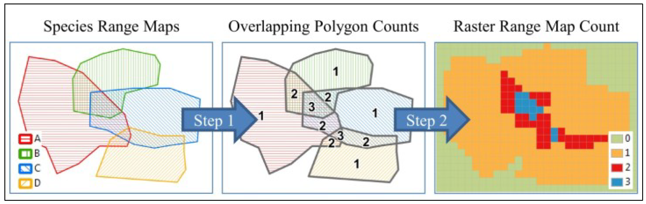
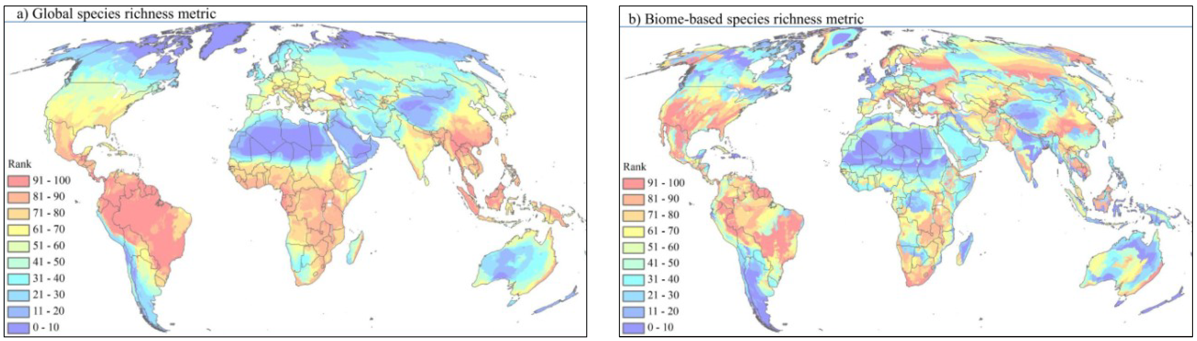
2.2. Species Richness Metric

We produced two species richness metrics based on the total number of species ranges overlapping a one km2 area using 28,000 International Union for Conservation of Nature (IUCN) range maps for vertebrate species [31] combined with an ecoregional plant richness dataset [32]. These combined data provided estimates of richness at a global-scale, which was also relativized by biome (see below) to account for latitudinal species richness gradient [39]. These two metrics facilitated comparison of richness both within and across climatic and vegetative zones.
To derive our range map counts, we removed marine-only species and those considered “extinct” or “extinct in the wild” as determined by IUCN, as well as any historical ranges. Remaining range maps were grouped by taxa (i.e., amphibians, birds, mammals and reptiles) and converted to raster using an overlapping polygon count procedure (Figure 1). The taxa groups were then summed together producing global values ranging from zero to 938. For plant richness, we performed a vector to raster conversion based on species count, which produced cell values ranging from zero to 10,000. Due to differences in the ranges of vertebrate and plant counts, we normalized values based on min/max normalization at a global-scale and by biome [40] before applying a spatial percentile-ranking to the summed product. Ranks were then rescaled from zero to 100 to produce final metric scores (Figure 2).
Figure 1. Range map overlapping polygon counts.
Sustainability 05 04444 g001
Step 1. Based on range maps for each taxa (i.e., amphibians, birds, mammals and reptiles), we ran a union analysis to produce a layer, which maintains the overall range of each species but also identifies the exact coincidence of overlapping ranges; Step 2. A unique id was created for each polygon based on the polygon centroid. All polygons with identical centroid id’s were then dissolved into one polygon with an attribute preserving the original coincidental polygon count. A final raster at a one km2 resolution was produced based on the dissolved polygons and the associated polygon count.
Figure 2. Species richness metrics.
Sustainability 05 04444 g002
Species richness metric based on (a) global and (b) biome ranking, which depicted areas most sensitive (red) to least sensitive (dark blue) to potential biodiversity impact. Most sensitive areas are regions globally or within a biome that display relatively high vertebrate and plant species range counts.

2.3. Threatened Species Metrics

We developed a threatened species metrics based on the number of IUCN red-listed species ranges classified as threatened. We relied again on IUCN vertebrate range maps [31] but only included those species designated as “critically endangered”, “endangered” or “vulnerable”. This selection resulted in 4682 species (1886 amphibians, 1219 birds, 1257 mammals, and 340 reptiles) out of the estimated total 28,000 mapped species. Again historical ranges were removed from analysis, as were marine-associated species. Following the overlapping polygon count procedure used for species richness (Figure 1), a raster was created per taxa calculating the number of threatened ranges overlapping a one km2 cell. All four taxa were then summed to produce an overall threatened species count with cell values ranging from zero to 59. A spatial percentile-ranking was then applied to both the overall threatened count and percent threatened value with both then being rescaled from zero to 100 (Figure 3).
Figure 3. Threatened species metrics.
Sustainability 05 04444 g003
Threatened species metric based on ranking the total count of threatened species. Areas most sensitive (red) to least sensitive (dark blue) to impact in relation to threatened species are depicted. Most sensitive areas are those regions with a relative high number of threatened vertebrate species.

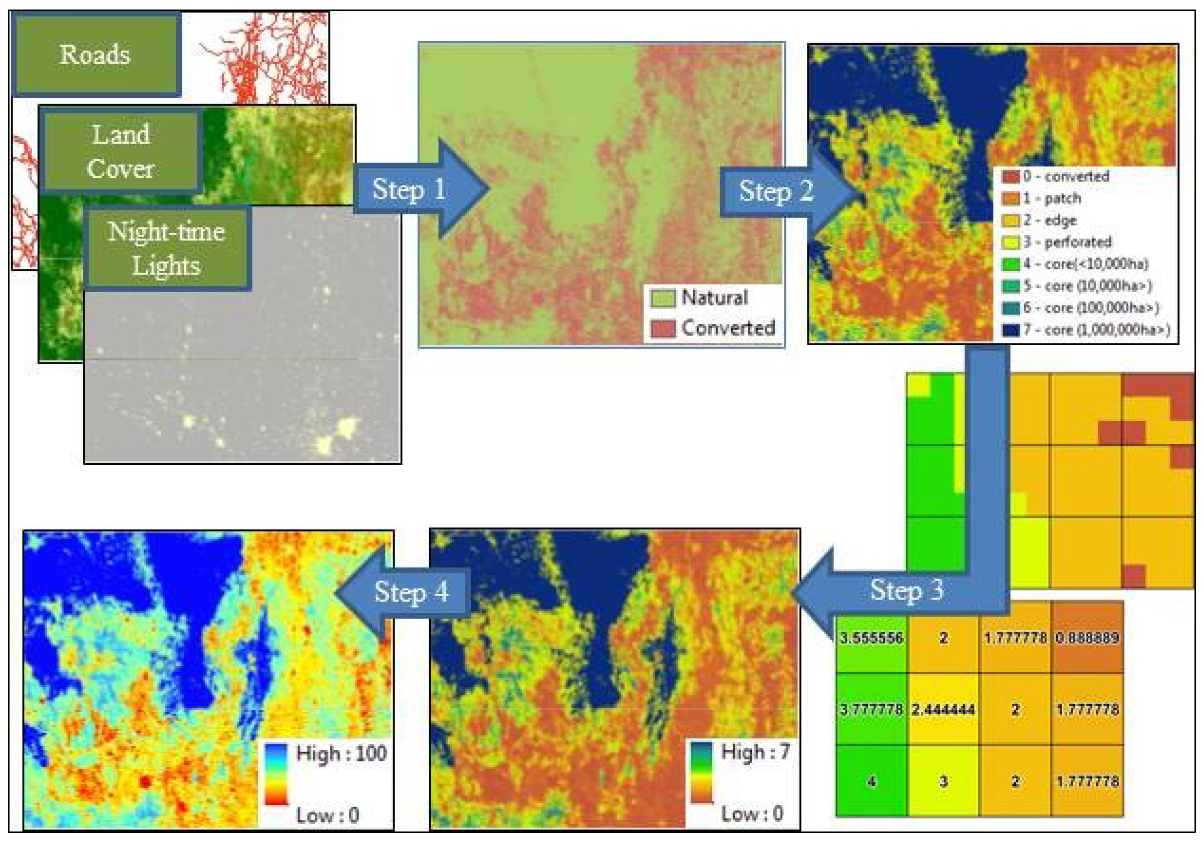
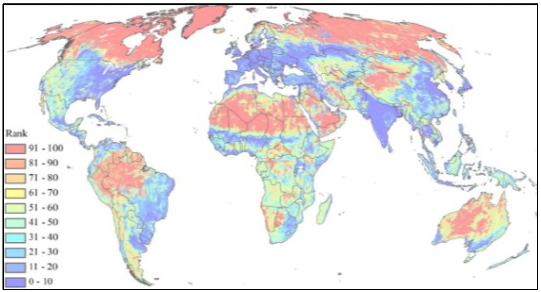
2.4. Habitat Intactness Metric

Using a four step process (Figure 4), we developed a metric that identifies levels of habitat intactness, with higher scores for contiguous, unaltered landscapes and low scores for highly human-altered areas. We used three global datasets: land cover [33], nighttime lights [34], and roads [35] and reclassified their associated cover types into binary classes—natural or converted. For the land cover dataset, areas identified as either cropland or urban were reclassified as converted while all other cover types (e.g., forest, grassland, shrub-land, wetlands), except water, were reclassified as natural. Lighted areas and roads were reclassified as converted, and areas without lights or roads as natural. These three binary layers were then combined to delineate natural versus converted landscapes.
To calculate levels of intactness of natural areas, we applied the Landscape Fragmentation Tool (LFT) [34]. The LFT tool measures habitat fragmentation and classifies target habitat types into four main categories—core, perforated, edge and patch—based on specified edge effects from anthropogenic disturbance [41]. Core areas of habitat are outside the edge effect and are not degraded from proximity to disturbance; edge and perforated areas occur along the periphery of habitat tracts containing core areas, with edges making up the exterior peripheries and perforated areas making up the interior edges along small gaps. Patches are small fragments that are completely degraded by the edge effect. We applied an edge-width of two kilometers, a distance used by other global analyses of habitat intactness [42,43] and supported by empirical fragmentation research [44,45,46]. We then applied the following ordinal ranking to the LFT output: 7: core areas > 1,000,000 ha, 6: 100,000 ha < core areas < 1,000,000 ha, 5: 10,000 ha < core areas < 100,000 ha, 4: core areas <10,000 ha, 3: perforated areas, 2: edges, 1: patches, and 0: converted areas (lacking natural habitats). Final habitat intactness scores were based on applying a spatial percentile-rank to a resampled, mean LFT score raster, which was then rescaled from 0 to 100 (Figure 5).
Figure 4. Habitat intactness metric processing steps.
Sustainability 05 04444 g004
Step 1. We combined land cover, roads, and night-time lights data to produce a binary raster of natural and converted areas (300 m resolution); Step 2. We analyzed levels of fragmentation of natural habitats using the Landscape Fragmentation Tool (LFT) based on a 2 km edge-width. We assigned resulting output to eight ordinal categories: 7: core areas > 1,000,000 ha, 6: 100,000 ha < core areas < 1,000,000 ha, 5: 10,000 ha < core areas < 100,000 ha, 4: core areas <10,000 ha, 3: perforated areas, 2: edges, 1: patches, and 0: converted areas; Step 3. We resampled our ranked LFT output to one km2 resolution and calculated the mean ordinal-ranked value; Step 4. A spatial percentile-rank was applied to the mean values and then rescaled from 0–100.
Figure 5. Habitat intactness metric.
Sustainability 05 04444 g005
The habitat intactness metric depicts areas most sensitive (red) to least sensitive (dark blue) to potential biodiversity impact based on levels of fragmentation of natural land cover. Most sensitive areas are located within large (greater than a million hectares), intact landscapes and the least sensitive areas are those landscapes that have been human altered. On average, any cell which was originally identified as part of any intact landscape (i.e., Landscape Fragmentation Tool output value equal to any type of core area) scored greater than 70.

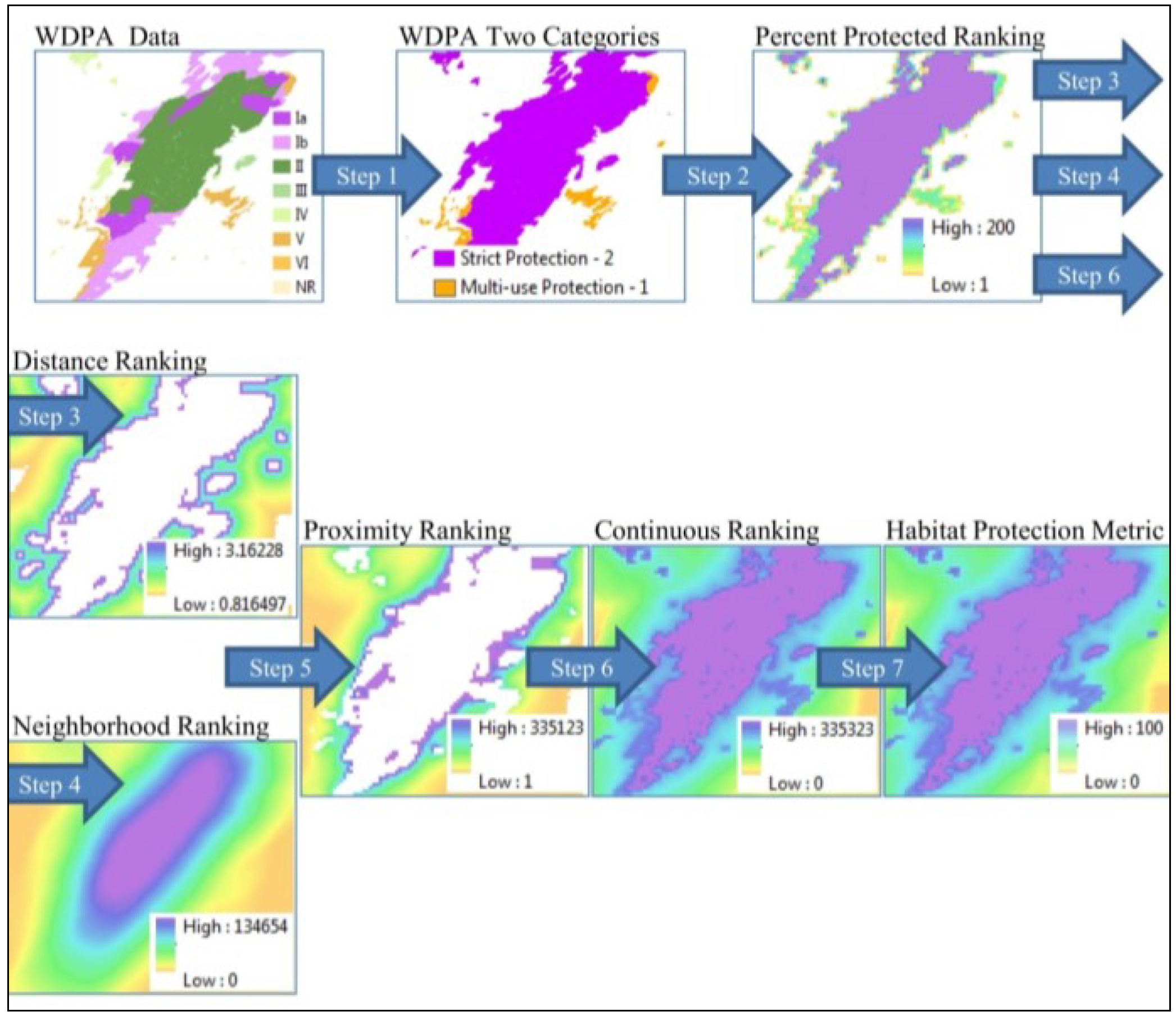
2.5. Habitat Protection Metric

We applied a seven step analysis (Figure 6) to the World Database of Protected Areas database (WDPA) [30] and developed a habitat protection metric based on the designation category of protected areas (PAs), the distance away from a PA, and the amount of land protected within a distance of potential influence. We considered only PAs with an IUCN status of “Adopted”, “Designated”, or “Inscribed” and excluded those which had an IUCN category listed as “Not Applicable” (e.g., Biosphere Reserves, RAMSAR sites, and World Heritage sites). These PAs listed as “Not Applicable” are areas of recognition, however they are usually broad areas made up of already existing protected areas having only have designation not legal status [47] and why we excluded them. Based on the IUCN category descriptions [48] and following McDonald and Boucher [49], we grouped PAs into strict (I-IV) or multi-use protection (V-VI and “Not Reported”). We then calculated the percentage of each one km2 cell that overlapped strict or multi-use PAs. To more heavily weight strict PAs, we doubled those percentages, which produced a ranked raster with values ranging from 200 (completely located within a strict PA) to 1 (1/100 of the cell intersects a multi-use PA).
Figure 6. Habitat protection metric processing steps.
Sustainability 05 04444 g006
Step 1. Using World Database of Protected Areas (WDPA), we categorized protected areas (PAs) into two protection classes (strict and multi-use) and removed all overlapping areas; Step 2. We ranked cells that intersect protected lands based on the percent of cell protected in one km2 area and type of protection by doubling strict PAs percentage values. This produced a raster with cell values ranging from a high score of 200 (completely located within a strict PA) to 1 (1/100 of the cell intersects a multi-use PA); Step 3. We created a distance ranking by applying an Euclidian distance routine from cells with a percentage protected and then inversely weighting the distanced value (i.e., closest cells having higher values) by applying the formula 100/square root (distance). This produced higher values being associated with cells closest to any cell having a portion already protected; Step 4. We produced a neighborhood ranking by applying a 15 km radius moving window analysis summing the percent protected ranking. This resulted in higher values for cells surrounded by or near large amounts of strictly protected lands; Step 5. We multiplied the distance ranking times the neighborhood ranking to produce and overall proximity ranking. This created a raster having higher values for cells closest to larger amounts of protected lands; Step 6. We combined the proximity ranking with the percent protected ranking to produce a continuous ranking raster. To insure that cells with any percentage of protected lands were ranked higher, we added the highest score from the proximity ranking to the percent ranking value before merging. Cells without a value were given a value of zero indicating they were not within 15 km of any protected area; Step 7. As a final step, we applied a spatial percentile-rank to the continuous ranking and then re-scaled these values from 0–100 to produce the final metric.
To rank cells outside of PAs, we used both a distance and a neighborhood ranking. For our distance ranking, we used 100/square root (distance). Our distance value was limited to being no greater than 15 km and was calculated by the Euclidian distance from any partial protected cells (i.e., percent protected rank raster). We selected 15 km distance because it is beyond the distance reported for majority of cumulative edge effects [45] and because most reporting guidance require that businesses recognize protected areas “near” their activities [13,15] but provide no distance guidance. To calculate the neighborhood ranking, we again used the percent protected rank raster but this time applied a moving window analysis with a 15 km window summarizing these percentage ranks. This gave us a raster distinguishing between those cells close to or surrounded by large amounts of strict protected lands versus those near isolated, small PAs. To obtain a final proximity ranking of all cells outside PAs, we multiplied the distance raster by neighborhood raster. This produced a raster with cells adjacent to or surrounded by large amounts of strictly protected lands being ranked the highest. Finally to create a continuous ranking for cells both occurring within, next to, and near PAs, we merged the percent protected raster with the neighborhood ranking raster. To insure those cells with any percent being protected ranked higher, we added the highest score from the proximity ranking to the percent ranking value before merging. A spatial percentile-rank was applied to this final continuous ranking raster with the output being then rescaled from 0–100 to produce the final metric (Figure 7).
Figure 7. Habitat protection metric.
Sustainability 05 04444 g007
The habitat protection metric depicting areas most sensitive (red) to least sensitive (dark blue) to biodiversity impact, based on the type of protection (i.e., strict protection or multi-use), distance to a protected area, and the amount of area protected. Most sensitive areas with scores of 100 are completely within a strict protected area versus areas with lowest scores (0) fall >15 km outside of a protected area. Those areas falling completely within multi-use areas or having over 50% of the cell overlapping a strict protected area scored at 90 or higher, and all other values (i.e., 89–50) were cells that were either on the border of protected areas or at least within 15 km of a protected area.

2.6. Application

Necessary to provide companies with the ability to use our biodiversity metrics would be an accompanying application. To obtain feedback on the potential use of such an application, we developed a prototype Internet mapping application that is being tested within The Nature Conservancy (TNC) (Figure 8). We designed the application to depict global environmental patterns and to help assess company sites (or their products or supply chain) in relation to species richness, threatened species, habitat intactness, and habitat protection without the need for in-house GIS expertise. The only requirement is for the user to have a list of sites and their associated locations (i.e., geographic coordinates in latitude and longitude). Output from the application provides users with the associated metrics for all sites uploaded. Additionally users can access custom reports for sustainability reporting (discussed below) as well as specific information provided by the original data providers to aid further site evaluation (e.g., threatened species list linking to IUCN website and/or protected area link to WDPA website). Currently this application is limited to TNC internal use only with the intent to make the application available for public usage pending permissions granted by original data sources.
Figure 8. Web map application.
Sustainability 05 04444 g008
Prototype Internet application to map company sites (or supply chains) and to provide metrics to rank them in terms of their potential biodiversity risk.

3. Business Application of Metrics

A company could use these biodiversity metrics (1) to gauge potential biodiversity sensitivity associated with their international facilities and to prioritize where they might conduct more detailed biodiversity action plans [9]; (2) to evaluate their products (or supply chain) in terms of potential biodiversity sensitivity and to inform when to conduct a more in depth life cycle assessment; and (3) to facilitate more consistent corporate sustainability reporting and provide answers to biodiversity questions within the Global Reporting Initiative (GRI).

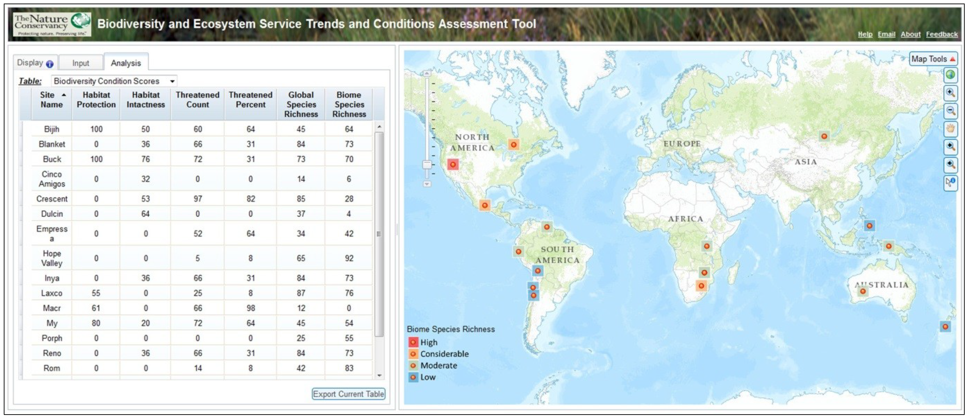
3.1. Site Portfolio Assessment

A company could use these biodiversity metrics to assess their facilities globally for potential biodiversity risks by uploading their sites within the application either manually or based on a pre-existing file of locations. A table listing all their sites with associated biodiversity metrics for each location would be produced (Table 1). With this table, a user can prioritize their sites based on any of our five metrics and group sites into categories of biodiversity risk based on their scores. For a biodiversity regulation risk assessment, companies could focus strictly on threatened species and habitat protection metrics and then expand to all five when examining potential reputational risks. In addition, users can merge this output with any additional information for their sites (e.g., land size, air emissions, waste volumes) for a more tailored biodiversity assessment. Currently within The Nature Conservancy’s (TNC) Smart Infrastructure Global Program, we are applying this methodology to help prioritize where to further our corporate engagements globally.
Table 1. Example site portfolio assessment, providing biodiversity scores to rank sites on any combination of metrics.
Site NameGlobal Species Richness ScoreBiome Species Richness ScoreThreatened Vertebrate ScoreHabitat Intactness ScoreHabitat Protection Score
A909668100100
B70951000
C768979072
D43791900
E68787468100
F957529077
G827168370
H827168370
I827168370
J50713800
K2459000
L34435500
M71416247100
N16368368100
O41310590
P8526985090
Q1550340
R14168076

3.2. Product Evaluation

A company could also use our metrics to evaluate potential biodiversity impacts of different suppliers or products in terms of where raw materials are sourced. This output would inform standards for green procurement, help select products and/or suppliers with less expected environmental sensitivity, and identify products to undergo a life cycle assessment. Similar to portfolio site assessment (as described above), raw material sourcing or manufacturing sites for products could be uploaded and biodiversity scores summarized/averaged for ranking purposes.

3.3. Corporate Sustainability Reporting

Sustainability reporting is how many in the business community highlight their biodiversity plans and outcomes. A widely adopted and well-accepted sustainability reporting framework is one developed by the Global Reporting Initiative (GRI), a non-profit organization that promotes economic, environmental and social sustainability [15]. Inherent to our metrics is the ability to use the source data (i.e., WDPA and IUCN) directly in answering questions EN11 and EN15 in the Global Reporting Initiative (GRI) sustainability report. Under GRI, a company must report on protected areas within close proximity (EN11) and on threatened species (EN15) at their sites. Through spatial overlay and proximity analyses, tables can be produced to support GRI reporting: (1) EN11 report on the number of protected lands (categorized by IUCN status) within 15 km of a site and the name, IUCN category, and distance of the closest protected area (Table 2); and (2) EN15 report on the number of red-listed species (and their IUCN status) at all sites (Table 3).
Table 2. Example output to answer EN11 within the Global Reporting Initiative sustainability report, which lists the number of protected areas ≤15 km of a site, grouped by IUCN category (i.e., Ia—Unreported), and information on the name, type, IUCN category, and distance of the closest protected area.
Site NameIaIbIIIIIIVVVIUnreportedClosest PA—NameClosest PA—TypeClosest PA—IUCN CatClosest PA—Distance (m)
A800033010Sekondi WaterworksForest ReserveNot Reported1,726
B70021000RavilevuNature ReserveIa255
C60140000Jaua SarisariñamaNational ParkII2,553
D200018700Manglares ChuruteEcological ReserveVI1,088
E21026203KakumNational ParkII1,913
F10000000GalibiNature ReserveIV14,573
G100015200Macizo AcahayNatural MonumentIII3,998
H101011500AbisuForest ReserveNot Reported2,203
I1001801010Esuboni ForForest ReserveNot Reported344
J000081200Laguna de los PozuelosNature MonumentIII1,092
K0000171200Los GlaciaresNational ParkII3,330
L00000300LanínNational ParkII380
M00020000Los AlercesNational ParkII12,905
N00001000CalileguaNational ParkII2,376
Table 3. Example output to answer EN15 within the Global Reporting Initiative sustainability report, which provides the total count of all IUCN vertebrate range maps overlapping a site, and the number of these range maps currently identified as threatened (i.e., Critical, Endangered, and Vulnerable).
Site NameCriticalEndangeredVulnerableTotal Threatened CountTotal Vertebrates Mapped by IUCN
A24814527
B2204250
C2204259
D22610426
E2158315
F21912424
G21912429
H1671497
I1438324
J1449325
K141116702
L14712526
M14510411
N13610514

4. Discussion

We developed five biodiversity metrics to help a company identify their sites where they may encounter the greatest environmental sensitivity in relation to species richness, threatened species, habitat intactness, and habitat protection. Although we view higher scores of all our metrics as areas with greater sensitivity to biodiversity impacts, we recognize that certain industries may not interpret and weight each metric equally. For this reason, we do not recommend one, overall biodiversity sensitivity assessment but rather suggest that business leaders use metric scores separately or in combination as they see best to derive their own tailored evaluation. For example, businesses near a protected area or in locations with high numbers of threatened species are likely to encounter regulatory restrictions that may constrain operations, which would be viewed as a potential risk. However, the potential to contribute funding to a local protected area, or to purchase or donate lands to buffer protection or to provide critical habitat for endangered species may be seen as an opportunity in a given region. These types of investments may provide corporate benefits in obtaining good will within a community and/or gaining the trust of local, environmental regulators.
We suggest that biodiversity metrics, such as the ones that we have developed, should be used in conjunction with other environmental and/or socio-economic data to better ensure a more complete biodiversity risk assessment. For example, we encourage companies to use measures of their direct and indirect footprint in combination with our biodiversity metrics. These may include the size of land used, the amount of resource needed, the amount of waste developed, amount of pollution generated, or the nature and intensity of direct and indirect land use changes. Additionally, companies can incorporate socio-economic indicators into biodiversity assessments, such a poverty, population levels, education levels of potentially impacted populations as these may influence the success of conservation actions by a company.

4.1. Appropriate Use

Like any data, our metrics have the potential for misuse especially when coupled with a mapping application that may foster a misperception that data will support a finer resolution analysis. Although our metrics have a resolution of one km2, the accuracy of the data supporting our biodiversity metrics requires that fine-scale siting decisions should be made with additional analysis and more local (field) data. Our metrics are intended to facilitate comparison between sites and not as definitive description of site level occurrences. We used a one km2 resolution, because it provides flexibility for aggregation of our metrics and decreased many of the artificial boundaries visible at courser resolution. Additionally, at a courser resolution, range map counts underlying our richness and threatened species metrics became inflated. Finally, a one km2 resolution does not support site-level analysis, but rather a relative, site-to-site comparisons and even this comparison should be used to apply relative categorical risks (e.g., high, medium, low) to sites based on natural breaks in the scores since there is relatively no difference in biodiversity sensitivity where scores are clustered close together.
Even though users can overlay metric values for a point location on a map, these values should not be interpreted as the biodiversity value at that specific site on the ground, but rather should be used only for comparison against other sites. For example, our threatened species metric relies on endangered species range maps, which relate to the general, spatial distribution of a species but does not indicate whether suitable habitat exists or whether that species is found specifically within a location. Additionally, we have worked with some companies to assess the validity of our biodiversity metrics by comparing our results to their previous assessments, we recognize the need to further validate the robustness of the metrics by having other companies assess these metrics and/or by doing a full validation analysis. Finally, while our metrics may help guide where companies should prioritize more extensive analysis, such an environmental assessment or biodiversity action plan, it is not recommended that they be used as the tool that would provide the data necessary to conduct these types of assessments.

4.2. Current Global Biodiversity Assessment Applications

Essential for corporations to become even more engaged in planning for biodiversity issues is not only providing them with the necessary data but also giving them the ability to easily use these data. Web-based tools such as Protected Planet [30], IUCN Red List of Threatened Species [31], Data Basins [50], and The Global Biodiversity Information Facility Mapping and Analysis Portal (GBIF_MAPA) [51] provide a wealth of biodiversity related information but require users to download and analyze these data to assess a potential or current site. While important in assessing a site for biodiversity, some companies have far too many locations to perform this kind of analysis on each of their current or future sites. While many large corporations retain environmental health and safety program with significant biodiversity experience many small to mid-size companies may lack staff with expertise to perform these basic tasks. It will also be critical to not only make the tool easy to use but to make access to the tool and metrics free of charge. Many small to mid-size companies have limited resources and they may forego biodiversity assessments if they divert financial resources.
Based on a recent survey of available biodiversity and ecosystem services tools [52], only two web-based mapping tools have been identified as global in scale and focusing specifically on synthesizing data provided from some of these previous sources to quickly assess biodiversity: IBAT and Normative Biodiversity Metric (NBM). IBAT provides users with detailed information and site comparisons for user-defined project boundaries based on counts of threatened species and distances to designated biodiversity areas and/or protected areas [52]. NBM uses a single metric, which combines pristineness and endangered species data to produce a biodiversity score [52]. NBM then provides users with the ability to digitize project boundaries to obtain scores relative to their current or future land holdings.
We see the need for a publicly-available tool that will provide companies with a quick pre-screening/ranking of all their sites based on potential biodiversity risk. Once sites have been identified as being sensitive to impacting biodiversity, additional regional/local data could be then used to provide a more detailed site assessment. For example, if a company has a portfolio of a hundred global sites providing them with the means to quickly identify sites with highest sensitivity to biodiversity will save them valuable time and resources while placing a priority on these sites.

5. Conclusions

Conservation scientists and practitioners have used regional and global conservation assessments to support and guide comprehensive and representative biodiversity protection [53,54,55]. In addition to identifying important places, these assessments help organize, update, and make available biodiversity information; develop, implement and prioritize strategies; evaluate success, and inform adaptive management of conservation investments and actions. The Nature Conservancy and its partners have completed over 150 ecoregional assessments around the world over the past 20 years. But many more ecoregions are in critical need of assessments. Using biodiversity metrics could help to ensure that investments made by companies are targeted at places in greatest need and assessments reflect land use changes that are important for both conservation and industry. In doing so, we hope to identify important synergies that will result in better conservation and business outcomes.

Acknowledgments

We thank Holly Copeland and Jen Molnar (The Nature Conservancy) for providing technical assistance; John DiMuro, Judy Gunderson and Mary Pudell (The Dow Chemical Company) for their consultation with the biodiversity sensitivity metrics and application development of BestCat; Mark Johnson (British Petroleum) and Gail Ross (Barrick Gold Corp.) for beta-testing BestCat and providing valuable feedback; Doe Cassidy, Michael Heiner, Mister Jinx and the people at Bean Cycle Coffee Shop for helpful discussions; and Bailey Oakleaf for his persistence and insistence for keeping it fun. Funding was provided by The Dow Chemical Company Foundation, The Nature Conservancy, Anne Ray Charitable Trust and The Robertson Foundation.

Conflicts of Interest

The authors declare no conflict of interest.

References

  1. Costanza, R.A.; Groot, R.; Farberk, S. The value of the world’s ecosystem services and natural capital. Nature 1997, 387, 253–260. [Google Scholar]
  2. Daily, G.C. Nature’s Services: Societal Dependence on Natural Ecosystems; Island Press: Washington, DC, USA, 1997; p. 392. [Google Scholar]
  3. Houdet, J.; Trommetter, M.; Weber, C. Understanding changes in business strategies regarding biodiversity and ecosystem services. Ecol. Econ. 2012, 73, 37–46. [Google Scholar]
  4. Rubino, M.C. Biodiversity finance. Int. Aff. 2000, 76, 223–240. [Google Scholar]
  5. Daily, G.C.; Ellison, K. The New Economy of Nature: The Quest to Make Conservation Profitable; Island Press: Washington, DC, USA, 2002. [Google Scholar]
  6. Armsworth, P.R.; Armsworth, A.N.; Compton, N.C.; Cottle, P. The ecological research needs of business. J. Appl. Ecol. 2010, 47, 235–243. [Google Scholar]
  7. Lovins, A.B.; Lovins, L.H.; Hawken, P. A road map for natural capitalism. Harv. Bus. Rev. 1999, 77, 146–158. [Google Scholar]
  8. Jeurissen, R.; Keijzers, G. Future generations and business ethics. Bus. Ethics Q. 2004, 14, 47–69. [Google Scholar] [CrossRef]
  9. Croucher, T.; Dholoo, E. To BAP or not to BAP? Challenges and opportunities in the adoption of biodiversity actions plans for the oil and gas sector. Soc. Petrol. Eng. 2010, 1, 1–6. [Google Scholar]
  10. McKenney, B.A.; Kiesecker, J.M. Policy development for biodiversity offsets: A review of offset frameworks. Environ. Manage. 2010, 45, 165–176. [Google Scholar]
  11. International Finance Corporation (IFC), International Finance Corporation Sustainability Framework; IFC: Washington, DC, USA, 2012.
  12. Rio Tinto. Rio Tinto’s Biodiversity Strategy. Available online: http://www.riotinto.com/documents/ReportsPublications/RTBidoversitystrategyfinal.pdf (accessed on 8 July 2013).
  13. Barrick Gold. Barrick Responsible Mining, Barrick Gold Sustainability Report 2010. Available online: http://barrickresponsibility.com/2010/en/online_pdf.html (accessed on 8 July 2013).
  14. Integrated Biodiversity Assessment Tool (IBAT). Available online: https://www.ibatforbusiness.org/login (accessed on 8 July 2013).
  15. Global Reporting Initiative (GRI). Biodiversity Sustainability Reporting Guidelines. Available online: https://www.globalreporting.org (accessed on 8 July 2013).
  16. Eichhorn, M.; Drechsler, M. Spatial trade-offs between wind power production and bird collision avoidance in agricultural landscapes. Ecol. Soc. 2010, 15. Article 10. [Google Scholar]
  17. Naughton-Treves, L.; Holland, M.B.; Brandon, K. The role of protected areas in conserving biodiversity and sustaining local livelihoods. Annu. Rev. Env. Resour. 2005, 30, 219–252. [Google Scholar] [CrossRef]
  18. Nelson, J.G. National parks and protected areas, national conservation strategies and sustainable development. Geoforum 1987, 18, 291–319. [Google Scholar] [CrossRef]
  19. Ray, J.C.; Ginsberg, J.R. Endangered species legislation beyond the borders of the United States. Conserv. Biol. 1999, 13, 956–958. [Google Scholar] [CrossRef]
  20. Jenkins, C.N.; Pimm, S.L.; Joppa, L.N. Global patterns of terrestrial vertebrate diversity and conservation. Proc. Natl. Acad. Sci. USA 2013. [Google Scholar] [CrossRef]
  21. Fletcher, R.J. Biodiversity conservation in the era of biofuels: Risks and opportunities. Front. Ecol. Environ. 2010, 9, 161–168. [Google Scholar] [CrossRef]
  22. Forman, R.T.; Sperling, T.D. Road Ecology; Island Press: Washington, DC, USA, 2003. [Google Scholar]
  23. Johnson, C.J.; Boyce, M.S.; Chase, R.L. Cumulative effects of human developments on Arctic wildlife. Wildlife Monogr. 2005, 160, 1–36. [Google Scholar]
  24. Vors, L.S.; Schaefer, J.A.; Pond, B.A.; Rodgers, A.R.; Patterson, B.R. Woodland caribou extirpation and anthropogenic landscape disturbance in Ontario. J. Wildl. Manage. 2007, 71, 1249–1256. [Google Scholar]
  25. Hoekstra, J.M.; Boucher, T.M.; Ricketts, T.H.; Roberts, C. Confronting a biome crisis: Global disparities of habitat loss and protection. Ecol. Lett. 2005, 8, 23–29. [Google Scholar]
  26. Loucks, C.; Ricketts, T.H.; Naidoo, R.; Lamoreux, J.; Hoekstra, J. Explaining the global pattern of protected area coverage: Relative importance of vertebrate biodiversity, human activities and agricultural suitability. J. Biogeogr. 2008, 35, 1337–1348. [Google Scholar] [CrossRef]
  27. White, R.P.; Murray, S.; Rohweder, M. Pilot Analysis of Global Ecosystems: Grassland Ecosystems; World Resources Institute: Washington, DC, USA, 2000. [Google Scholar]
  28. Hannah, L.; Carr, J.L.; Lankerani, A. Human disturbance and natural habitat: A biome level analysis of a global data set. Biodivers. Conserv. 1995, 4, 128–155. [Google Scholar] [CrossRef]
  29. Chape, S.; Blyth, S.; Fish, L.; Fox, P.; Spalding, M. 2003 United Nations List of Protected Areas; IUCN, Gland, Switzerland and Cambridge, UK and UNEP-WCMC: Cambridge, UK, 2003. [Google Scholar]
  30. The World Database on Protected Areas (WDPA). Available online: http://www.protectedplanet.net (accessed on 8 July 2013).
  31. IUCN Red List of Threatened Species, Version 2012.1. Available online: http://www.iucnredlist.org (accessed on 8 July 2013).
  32. Kier, G.; Mutke, J.; Dinerstein, E.; Ricketts, T.H.; Küper, W.; Kreft, H.; Barthlott, W. Global patterns of plant diversity and floristic knowledge. J. Biogeogr. 2005, 32, 1107–1116. [Google Scholar] [CrossRef]
  33. GlobCover Land Cover v2 2008 database. Available online: http://ionia1.esrin.esa.int/index.asp (accessed on 8 July 2013).
  34. Nighttime Lights of the World 2010. Available online: http://sabr.ngdc.noaa.gov (accessed on 8 July 2013).
  35. Global Roads Database. Available online: http://sedac.ciesin.columbia.edu/data/set/groads-global-roads-open-access-v1 (accessed on 8 July 2013).
  36. Snyder, J.P. Map Projections—A Working Manual. Available online: http://pubs.er.usgs.gov/publication/pp1395 (accessed on 8 July 2013).
  37. May, K.; Nicewander, W.A. Reliability and information functions for percentile ranks. J. Educ. Meas. 1994, 31, 313–325. [Google Scholar] [CrossRef]
  38. Crocker, L.; Algina, J. Introduction to Classical and Modern Test Theory; Harcourt Brace Jovanovich College Publishers: New York, NY, USA, 1986. [Google Scholar]
  39. Koleff, P.; Gaston, K.J. Latitudinal gradients in diversity: Real patterns and random. Consels. Ecography 2001, 24, 341–351. [Google Scholar]
  40. Olson, D.M. Terrestrial ecoregions of the world: A new map of life on earth. BioScience 2001, 51, 933–938. [Google Scholar] [CrossRef]
  41. Vogt, P.; Ritters, K.H.; Estreguil, C.; Kozak, J.; Wade, T.G.; Wickham, J.D. Mapping spatial patterns with morphological image processing. Landsc. Ecol. 2007, 22, 171–177. [Google Scholar] [CrossRef]
  42. UNEP, GLOBIO: Global Methodology for Mapping Human Impacts on the Biosphere; UNEP: Nairobi, Kenya, 2002.
  43. Sanderson, E.W.; Jaiteh, M.; Levy, M.A.; Redford, K.H.; Wannebo, A.V.; Woolmer, G. The human footprint and the last of the wild. BioScience 2002, 52, 891–904. [Google Scholar] [CrossRef]
  44. Alkemade, R.; Oorschot, M.; Miles, L.; Nellmann, C.; Makkenes, M.; Brink, B. GLOBIO3: A framework to investigate options for reducing global terrestrial biodiversity loss. Ecosystems 2009, 12, 374–390. [Google Scholar] [CrossRef]
  45. Broadbent, E.N.; Asner, G.P.; Keller, M.; Knapp, D.E.; Oliveira, P.J.C.; Silva, S.N. Forest fragmentation and edge effects from deforestation and selective logging in the Brazilian Amazon. Biol. Conserv. 2008, 141, 1745–1757. [Google Scholar] [CrossRef]
  46. Benítez-López, A.; Alkemade, R.; Verweij, P.A. The impacts of roads and other infrastructure on mammal and bird populations: A meta-analysis. Biol. Conserv. 2010, 143, 1307–1316. [Google Scholar] [CrossRef]
  47. Chape, S.; Spalding, M.; Jenkins, M.D. The World’s Protected Areas; UNEP World Conservation Monitoring Centre, University of California Press: Berkely, CA, USA, 2008. [Google Scholar]
  48. Dudley, N. Guidelines for Applying Protected Area Management Categories; IUCN: Gland, Switzerland, 2008. [Google Scholar]
  49. McDonald, R.I.; Boucher, T.M. Global development and the future of the protected area strategy. Biol. Conserv. 2011, 144, 383–392. [Google Scholar] [CrossRef]
  50. Data Basins. Conservation Biology Institute. Available online: http://databasin.org (accessed on 8 July 2013).
  51. Global Biodiversity Information Facility (GBIF). Available online: http://www.gbif.org (accessed on 8 July 2013).
  52. World Business Council for Sustainable Development (WBCSD). Eco4Biz—Ecosystem services and biodiversity tools to support business decision-making. Available online: http://www.wbcsd.org/eco4biz2013.aspx (accessed on 8 July 2013).
  53. Cowling, R.M.; Pressey, R.L. Introduction to systematic conservation planning in the Cape Floristic Region. Biol. Conserv. 2003, 112, 1–13. [Google Scholar] [CrossRef]
  54. Noss, R.F. A checklist for wildlands network designs. Conserv. Biol. 2003, 17, 1270–1275. [Google Scholar] [CrossRef]
  55. Groves, C.R. Drafting a Conservation Blueprint: A Practioner’s Guide to Planning for Biodiversity; Island Press: Washington, DC, USA, 2003; p. 457. [Google Scholar]

