Article

Shared Urban Greywater Recycling Systems: Water Resource Savings and Economic Investment

1
Civil Engineering/College of Engineering and Physical Sciences, University of Birmingham, Birmingham B152TT, UK
2
International Synergies, 44 Imperial Court, Kings Norton Business Centre, Pershore Road South, Birmingham B30 3ES, UK
*
Author to whom correspondence should be addressed.
Sustainability 2013, 5(7), 2887-2912; https://doi.org/10.3390/su5072887
Submission received: 28 April 2013 / Revised: 6 June 2013 / Accepted: 21 June 2013 / Published: 3 July 2013

Abstract

:
The water industry is becoming increasingly aware of the risks associated with urban supplies not meeting demands by 2050. Greywater (GW) recycling for non-potable uses (e.g., urinal and toilet flushing) provides an urban water management strategy to help alleviate this risk by reducing main water demands. This paper proposes an innovative cross connected system that collects GW from residential buildings and recycles it for toilet/urinal flushing in both residential and office buildings. The capital cost (CAPEX), operational cost (OPEX) and water saving potential are calculated for individual and shared residential and office buildings in an urban mixed-use regeneration area in the UK, assuming two different treatment processes; a membrane bioreactor (MBR) and a vertical flow constructed wetland (VFCW). The Net Present Value (NPV) method was used to compare the financial performance of each considered scenario, from where it was found that a shared GW recycling system (MBR) was the most economically viable option. The sensitivity of this financial model was assessed, considering four parameters (i.e., water supply and sewerage charges, discount rate(s), service life and improved technological efficiency, e.g., low flush toilets, low shower heads, etc.), from where it was found that shared GW systems performed best in the long-term.

1. Introduction

Population growth, rapid urbanization, higher standards of living and climate change influence greatly the growth of urban water consumption [1]. International Water Management Institute [2] projected that total global urban water consumption will increase from 1995 to 2025 by 62%. In the UK, the government’s Water White Paper [3] warned that climate change and population growth were increasingly likely to lead to water shortages by 2050. This would have a significant impact on ‘liveability’ in urban areas, not the least of which is city centre landscapes, and throws up many quality of life issues for an individual. In response to this, the Environment Agency advocated a radical overhaul of current water management strategies in order to prevent such a catastrophic occurrence [4,5]. There are two ‘key’ approaches that could be adopted to ensure that the urban water supply/demand balance is met—by 2050. The first approach is to develop additional supplies, locally where possible or nationally as required, for example: deep groundwater abstraction, new dams and reservoirs, seawater desalination and importing water from greater distances [6]. However, in many cases, these additional sources are either unavailable or would need to be developed at extremely high direct and indirect costs compared with existing water resource options. The second approach is to maintain existing supply sources and seek to reduce potable water demands through: (i) optimizing the existing water supply system (i.e., reducing leakage), installing water-saving devices and/or changing public behaviour; (ii) water re-use; and (iii) water recycling [7,8,9].
Greywater (GW) recycling (iii above) is receiving increasing attention as part of an overarching urban water management plan [9,10,11]. Where GW is defined as the wastewater from baths, showers, handbasins, washing machines, dishwashers and kitchen sinks and excludes streams from toilets [12]. There are numerous case studies of installed GW systems within individual family dwellings, multiple housing dwellings, multi-storey office buildings and individual (multi-room) hotel buildings [13,14,15,16,17,18,19,20,21,22,23,24,25]. Toilet flushing is a frequently cited GW application. Not least because toilet flushing in a typical home accounts for approximately 30% of home water use and can reach over 60% in offices [26]. The high volume of GW generation in domestic properties, which accounts for approximately 50 to 70% of daily water outflow, is usually greater than the requirement for GW use (i.e., toilet flushing which requires 20 to 36% water inflow) [27] In other words, there would be a substantial excess of GW remaining (up to 50% of the GW produced) once toilet flushing demands are met through GW supplies. In contrast, the GW produced in commercial, retail and other non-residential buildings, which accounts for approximately 21% of water outflow (from hand basins alone), is substantially less than the requirement for GW use (i.e., toilet flushing, which requires 43 to 65% water inflow). In other words, a deficit of GW exists; hence, the cost of the infrastructure and treatment equipment is unlikely to justify the long pay-back periods under current water pricing [28,29]. Although, this is very much influenced by the type of GW treatment system adopted [30].
This paper presents an innovative method to improve the efficiency of urban GW recycling systems through adopting a symbiosis approach; GW in mixed-use developments is shared between different users. The mixed-use development has perhaps the best potential for GW systems: because the accommodation buildings (e.g., residential, hotels, student halls of residence) produce more GW than they need and the excess can be re-used in other types of buildings where GW production is lower than demands (e.g., offices or retail buildings). In this specific case, the shared GW generation and use from domestic dwellings and offices (and their respective demands) is maximised to make the system much more viable, economically (in terms of £ saved) and environmentally (in terms of preservation of a valuable limited natural resource). This paper compares total costs using Net Present Value (NPV) and water savings across five different supply/demand scenarios with different GW treatment options (see Section 2.1). The sensitivity analysis considers the impact of water and wastewater prices, discount rate(s), service life and technological efficiency of micro-components in buildings. A discussion of the results is provided and conclusions subsequently drawn.

2. Water Resources: Supply and Demand for GW Scenarios

In this section, five scenarios for water supply and treatment are outlined (Section 2.1), a description of the residential and office building(s) is provided (Section 2.2) and the respective water demands and potential for GW production determined (Section 2.3). Throughout, it is assumed that GW is substituted only for water closet (WC) flushing. Whilst GW can be used for other purposes (e.g., gardening, car washing), these are beyond the scope of this current paper. In terms of water utility infrastructure requirements, all scenarios are consistent with the 2011 UK Building Regulations [31], which specify metering for all new properties, six litres/flush for standard toilets and no more than 7.5 litres/bowl/hour for standard urinals. The technological efficiency of water using appliances and respective water using behaviour is discussed in detail for domestic properties and offices in Section 2.3.1 and Section 2.3.2, respectively. The treatment performances of MBR and VFCW are well-reported within the literature (e.g., [30,32]) and, therefore, will not be repeated here.

2.1. Defining GW Recycling Scenarios

The five scenarios analysed in this paper are listed below and shown in Figure 1. A short description of each follows.
Scenario 1:
Mains supply scenario (no greywater)
Scenario 2a:
Individual GW recycling system (with GW treatment via MBR)
Scenario 2b:
Individual GW recycling system (with GW treatment via VFCW)
Scenario 3a:
Shared GW recycling system (with GW treatment via MBR)
Scenario 3b:
Shared GW recycling system (with GW treatment via VFCW)
Figure 1. Various water supply scenarios (WTP, water treatment plant; WWTP, waste water treatment plant; potable mains water flows shown by blue line; greywater (GW) flows shown by dotted line; blackwater (BW) flows shown by black lines).
Sustainability 05 02887 g001
In Scenario 1 (Figure 1a), it is assumed that the current practice for water supply and wastewater removal occurs, i.e., centralised supply and treatment. Whilst GW is undoubtedly produced, it is neither collected nor recycled for reuse for standard toilets and urinals within either building. Figure 1a shows the respective flows of water for Scenario 1.
In Scenario 2a and 2b (Figure 1b), distinction is made between potable and non-potable water supplies. Within the residential building, it is assumed that GW is collected from showers only and used for flushing standard toilets. Initial estimations (Table 1) show that this supply source more than meets demands; therefore, GW from basin and baths is not required. In office buildings, the only source of GW is from hand basins, which is subsequently used to flush standard toilets and urinals. In Scenario 2a, it assumed that a Membrane Bioreactor (MBR) is used to treat GW, whilst in Scenario 2b, a vertical flow constructed wetland (VFCW) is adopted. Figure 1b shows the respective flows of water for Scenario 2a and 2b.
Table 1. Assumed residential and office building descriptions [26,33,34].
VariablesResidential blockOffice block
Number of floors 10 a7
Total floor area (m2)10,24013,860
(Per floor)(1,024)(1,980)
Occupants/Employees432 b,c924 d
(Per floor)(43)(66 males and 66 females)
Total number of toilets180 e63 f
(Number of toilets/floor)18e(3 male, 5 female, 1 disabled) f
Total number of urinalsN/A14 g
(Number of urinals/floor)(2)
a 3 m floor heights; b assuming 2.4 occupants per flat; c based on 57 m2 average UK room size in high-rise buildings [33]; d assuming one employee per 15 m2 [25] ; e assuming one toilet per flat; f assuming one toilet per 14 female employees and one toilet per 25 male employees, plus one disabled toilet per floor [34]. assuming one urinal per 33 male employees.
In Scenario 3a and 3b (Figure 1c), GW is collected from residential showers and handbasins and treated at one shared treatment unit, then recycled for WC and urinal flushing in both office and residential buildings. In Scenario 3a, it is assumed that a membrane bioreactor (MBR) is used to treat GW. In Scenario 3b, a vertical flow constructed wetland (VFCW) is used to treat GW. Figure 1c shows the respective flows for Scenario 3a and 3b.

2.2. Description of Mixed-Use Buildings Sharing GW

To develop a generalized model, this paper firstly adopts then analyses a recently constructed multi-storey residential building and office building. The various dimensions adopted within this study were adopted directly from the Birmingham Eastside mixed-use development—an area where innovative sustainability systems were being considered in the visioning stages of planning [35,36] The various data relating to each building are presented in Table 1.
The general layout of the building(s) is shown in Figure 2. The cross-connection distance between office block and residential block is 100 m, and it is assumed that both buildings would be connected to the municipal central water supply and wastewater treatment plant. Sizing of pipes (Figure 2) is based upon BS EN 806-4 (guidelines for piping in buildings) and BS6700 (recommended design flow rates). The impact of changing cross-connection distance, number of floors and floor area are not considered here.
Figure 2. Dimensions (not to scale) of mixed-use building(s) under analysis (schematic for pipe work within Scenario 3a (see later) is shown). MBR, membrane bioreactor.
Sustainability 05 02887 g002

2.3. Water Demands and GW Production

In order to estimate likely greywater volumes produced and consumed in domestic residencies and offices, we need to consider the breakdown of total water demands by end-use. As the focus of this study is on UK residential and office high-rises in urban mixed-use areas, internal demands only are included. The associated impact of changes to these input parameters on supply demand requirements is beyond the focus of this paper. For further information, see Hunt et al. [8]. Total daily water consumption due to garden watering is excluded. Non-potable demands in offices and domestic dwellings are highly dependent on WC type (e.g., water flush, air flush and composting), size of cistern adopted (i.e., nine to zero litres/flush) and changes to user behaviour. The effects of these are discussed further in Section 4.2.4.

2.3.1. Water Demands in Domestic Dwellings

The water demands for a typical domestic resident can be seen in Figure 3 and Table 2. The data for predicted frequency of uses and volume of water per use are based on past monitoring studies [37,38,39,40,41,42,43]. The calculated water demand value of 148 litres/person/day reflects the average per capita water use in the UK domestic sector [41] (Table 2). Water demands (and greywater generation) within the residential high-rise are calculated by multiplying frequency of appliance(s) use by volume of water consumption (per use) by the number of occupants (Table 1). This assumes a linear relationship between frequency of water use and occupancy. Such an approach has been successfully adopted by many authors, including [8,38,43]. It is assumed that each flat has one toilet, one hand basin and one shower connected to the GW system. Occupancy rates are based on UK average values, as previously adopted by [8,41,43]. Operation is assumed to be for 365 days per year.
Figure 3. Water usage breakdown by end-use in UK residential dwellings, GW production highlighted. WC, water closet.
Sustainability 05 02887 g003
Table 2. Water usage breakdown in residential dwellings [37,38,39,40,41,42,43].
Water useWater consumption (units)Duration of use (minutes/ usage)Frequency of use (per day & person)Total water use (Litres/day/person)Fate of streams
WC flushing6 (L/usage)-4.828.8to sewer
Hand basin8 (L/minute)0.333.59.2to GW recycling
Washing machine80 (L/load)-0.2116.8to sewer
Shower12 (L/minute)80.657.6to GW recycling
Bath116 (L/usage)-0.1618.6to GW recycling
Kitchen sink8 (L/minute)0.333.59.2to sewer
Dishwasher24.9 (L/usage)-0.235.7to sewer
Other 2 (L/day/person) 2to sewer
Total daily water consumption (L/person/day)148

2.3.2. Water Demands in Offices

The water demands for a typical office resident can be seen in Table 3 and Figure 4. The data for predicted frequency of uses and volume of water per use are based on past monitoring studies [26,44]. The calculated value of 15 litres/person/day for male employees and 19.4 litres/person/day for female employees reflects the average per capita water use in the UK offices [26]. Based on the findings of Waggett and Arotsky [26], there is assumed to be one employee for every 6.7 m2, and based on the British Council for Offices Guide 2000, a value of 15 m2 is suggested; the lower density value is adopted here. The 15 m2 and ratio of male and female employees is 1:1 [34]. Hence, there is a direct relationship between floor area and water demand per employee that can be used. Frequency of WC flushing in female toilets is assumed to be two-times higher than in male toilets. This is based on the fact that male toilet facilities include urinals in addition to WC’s. Flushing system for urinals are assumed to operate 12 hours per day, five days per week (assuming water saving timers are fitted) and not 24/7, based on water regulations [45]. Frequency of hand basin use is assumed to be higher in female toilets than in male toilets based on the monitoring study by Thames Water‘s―Watercycle project at the Millennium Dome, UK [44]. For cleaning purposes, it is assumed that each toilet and urinal flushes twice, and each hand basin runs for five seconds. The respective water usage breakdown for both male and female employees in the UK is presented in Table 3. The number of toilets, urinals and hand basins for offices is assumed to be one per 25 males and one per 14 female employees, plus an extra one for persons with disability [36]. Offices are assumed to be in operation 261 days per year.
Table 3. Water usage breakdown for male and female office employees (Italics shows where female water usage differs).
Water useWater consumption (units)Duration of use (minutes/usage)Frequency of use (per day & person)Total water use (Litres/day/person)Fate of streams
WC flushing6 (lit/flush)-1 (2)6 (12)to sewer
Urinal3.6 (lit/bowl/hr)a-1 (0)3.6 (N/A)to sewer
Hand basin8 (lit/min)0.22 (3)2.5 (3.8)to GW recycling
Kitchen sink8 (lit/min)10.10.8to sewer
Cleaning12.6 (lit/clean)--1.0 (1.8)to sewer
Canteens1 (lit/day/person)--1.0to sewer
Total daily water consumption (l/employee/day)15 (19.4)
a Male urinals have a certain flush volume per urinal bowl (i.e., there is typically one water cistern that will service multiple bowls—when it flushes, all bowls are flushed simultaneously). The bowls are then (typically) flushed at set time intervals during the day. 2011 UK Building Regulations [31] specify urinals should use no more than 7.5 litres/bowl/hour and should be considered to operate 12 hours per day, five days per week (assuming water saving timers are fitted) and not 24/7, based on UK Water Regulations pre-2011.
Figure 4. Water usage breakdown in UK offices, GW production highlighted [26,34,44].
Sustainability 05 02887 g004

2.3.3. GW Sharing Potential between Offices and Residential

From Table 2 and Figure 5, it can be seen that daily domestic greywater production per person (9.2 + 57.6 + 18.6 L/person/day) is much higher than greywater demands for WC flushing (28.8 L/person/day), whilst daily office greywater production per male and female employee (6.3 L/two-employees/day) is significantly less than greywater demands (21.6 L/two-employees/day). However, it can be seen also that excess daily domestic GW generation (56.6 L/person/day) can more than meet daily office greywater deficits (15.2 L/two-employees/day). In fact, the excess greywater produced from one domestic resident will approximately meet the greywater demands of four office employees (two males and two females); therefore, cross-connection appears to be a sensible approach based on flow volumes at the individual scale. The ability of supplies to meet demands at high-rise scale will ultimately depend on the ratio of domestic residents to office employees.

3. Economic Analyses

3.1. Assessing Financial Performance

In general, the aspects that need to be taken into account when evaluating the financial performance of a GW recycling system are the savings and expenses (CAPEX and OPEX). The financial performance module, as adopted within this Chapter, is shown in Figure 6.
Data and information uses in this research were obtained from a variety of sources including:
  • Literature (e.g., journal papers, conference papers, water manuals)
  • Researchers currently active or previously active in the field
  • Private sector companies
It is assumed that economic conditions are similar through the life time of the system. In reality, world events, like global recession, will significantly affect the world economy. In addition, electricity and water prices have been assumed to change in the predicted inflationary market manner, rather than being rapid and disordered, as perhaps the result of shock events.
Figure 5. Greywater production and consumption for a single domestic resident and two office employees (one male + one female).
Sustainability 05 02887 g005
Figure 6. Financial performance module. CAPEX, capital cost; OPEX, operational cost; NPV, Net Present Value.
Sustainability 05 02887 g006

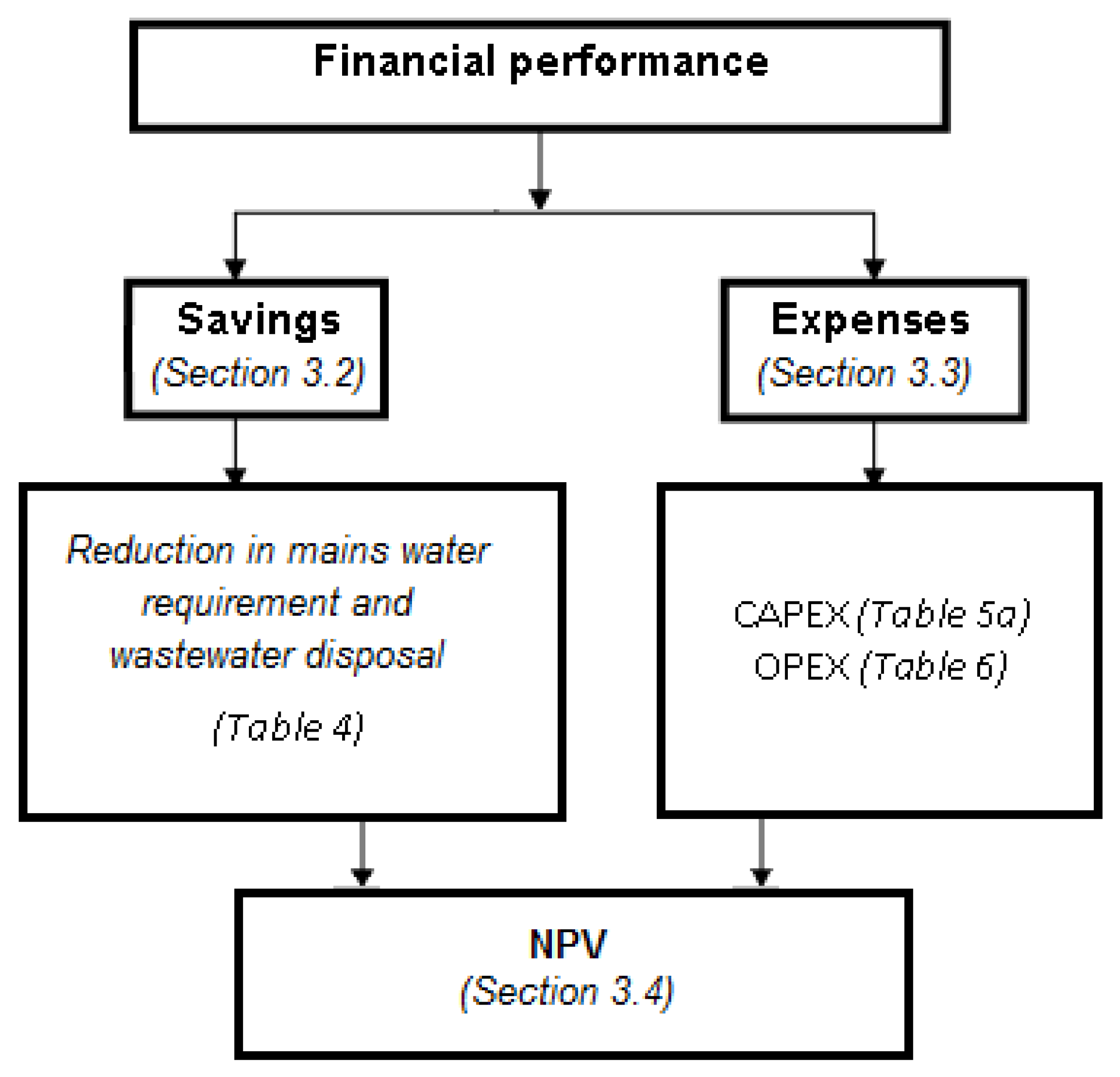
3.2. Savings: Main Water and Wastewater

Models that include a financial factor typically use the cost savings in main water supply (i.e., due to replacement with recycled GW) and wastewater disposal (i.e., due to reduced outflow requirements) as the main indicator of financial performance. These are commonly referred to as avoided costs and are the primary ways in which GW recycling systems offer the potential to save money on a private basis [21,46,47].
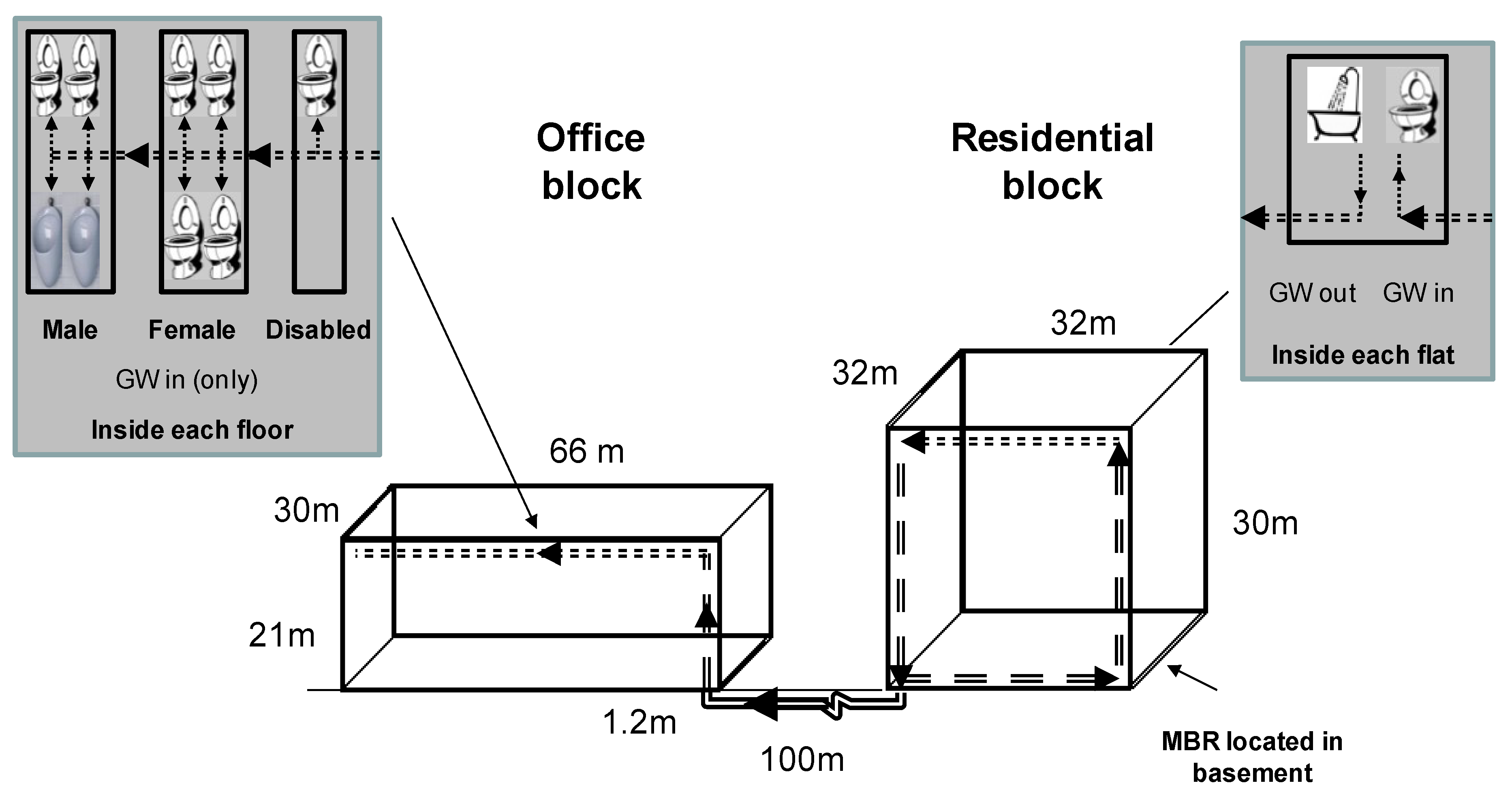
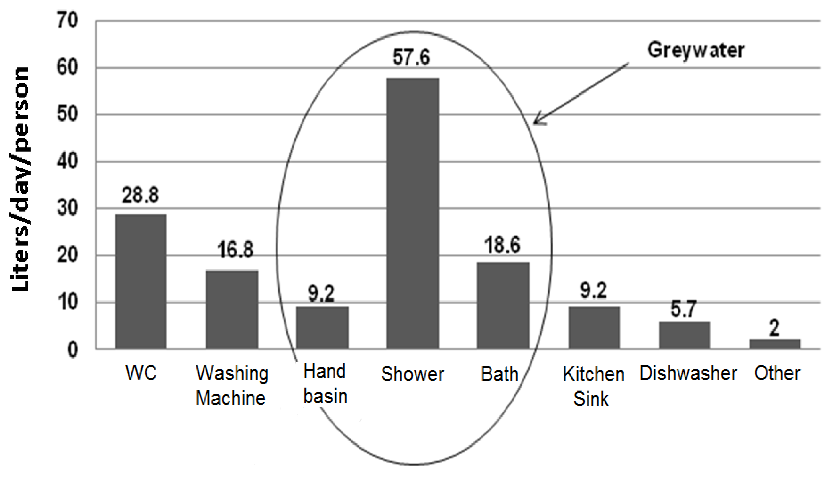
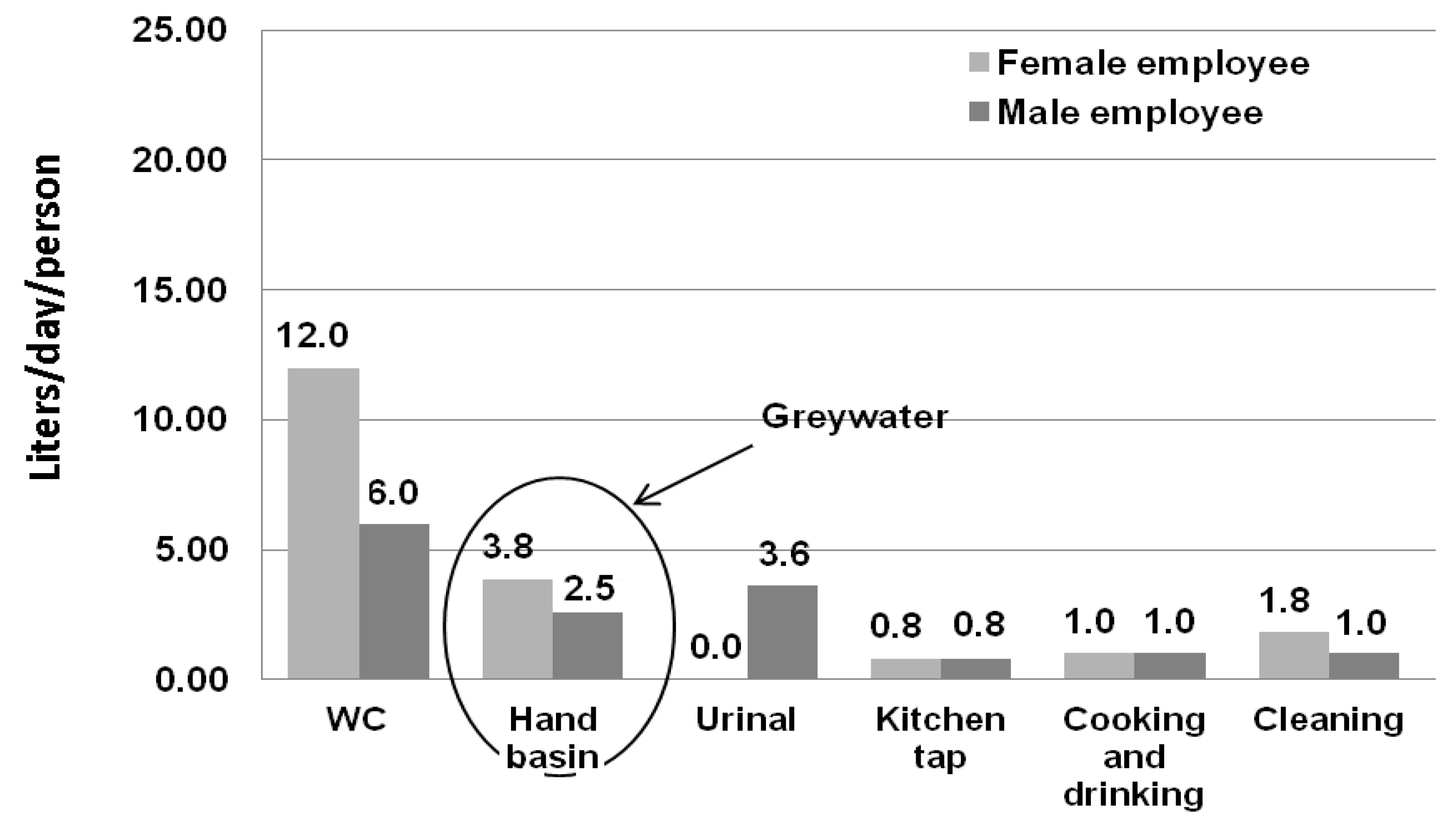
The simulation results from the following water flow module are used to provide quantification of the water saving potential for the mixed-use GW recycling system. The module has two components: annual GW supply (GWS) and annual GW demand (GWD). Equations 1 and 2 are used to calculate the volume of GW supply in residential (GWSR) and office block (GWSO). The GW supply component is contributed to from showering within the residential block and from hand basin(s) within the office block. (Other sub components, e.g., bathing, or washing machines, could be added by the user if so desired, but are not considered here.)
The input data for these equations is shown in Table 2, Table 3.
GWSR = Vs × Fs × R × T
where:
  • Vs = total shower volume (l/use),
  • Fs = frequency of shower (uses/person/day),
  • R = number of residents, and
  • T = number of days used per year.
GWSO = VB × FB × E × T
where:
  • VB = total hand basin volume (l/use),
  • FB = frequency of hand basin use (uses/employee/day),
    E = number of employees (male or female),
[Please note for Scenarios 3a and 3b, GWSO is not included within the analysis (
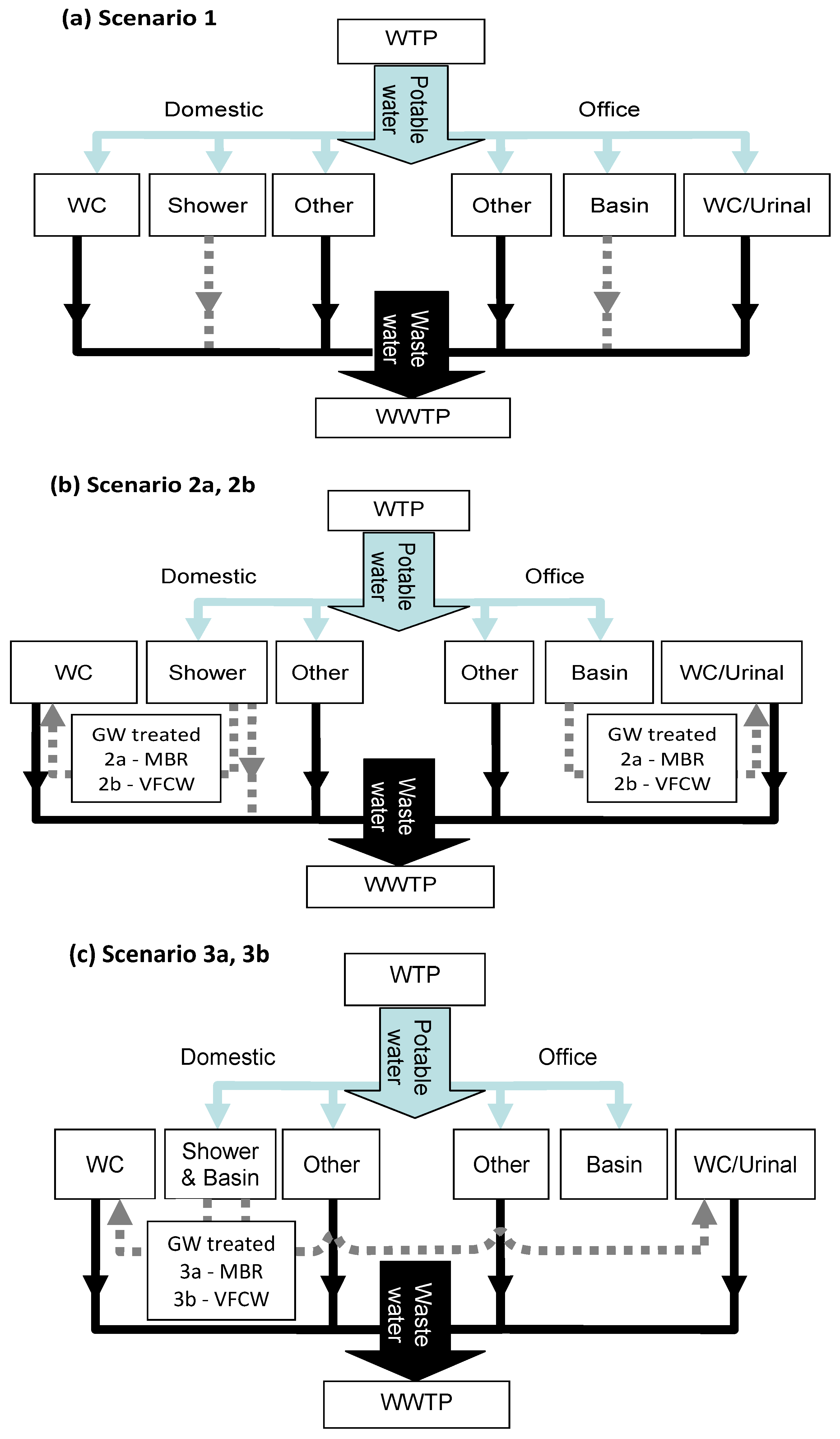
Figure 1c); hence, the total GW supply comes from Equation 1.]
The second component of the water flow module is for greywater demand. It is assumed that greywater is only used for toilet/urinal flushing. The total greywater demand for toilet flushing in residential (GWDR) and toilet and urinal flushing in offices (GWDO) is calculated by using Equation 3 and Equation 4:
GWDR = VT × FT × R × T
where:
  • VT = volume of toilet flush (l/flush),
  • FT = frequency of toilet flush (uses/person/day),
GWDO = (VT × FT × E + Vu × N × H) × T
where:
  • Vu = volume of urinal (lit/bowl/hr),
  • N = number of urinals in building,
  • H = hours of use per day.
[Please note the total demand in shared Scenarios 3a and 3b is found through the summation of GWDR and GWDO, i.e., Equations 3 and 4.].
Equation 4 can be used for calculating the toilet flushing demand for female employees without considering the urinal flushing. The net volume of saved water (Ws) and wastewater (WWs) is then calculated using Equations 5 or Equation 6:
If GWS > GWD then Ws = GWD, and WWs = GWD
If GWS < GWD then Ws = GWS, and WWs = GWS
The value of water saved (S) is calculated using Equation 7:
S = (Ws × WP) + (WWs × WWP)
where WP is the price of the main water and Ws is the volume of GW used. WWP is the wastewater disposal cost, and WWs is the reduction in wastewater outflow. The ratio between water demand and wastewater generation is assumed stable at 0.98.
The various daily total flow rates for water (i.e., the cumulative flows from both the office and residential blocks) and associated yearly costs/savings are shown in Table 4. It can be seen that the highest potable mains water demands (79.8 m
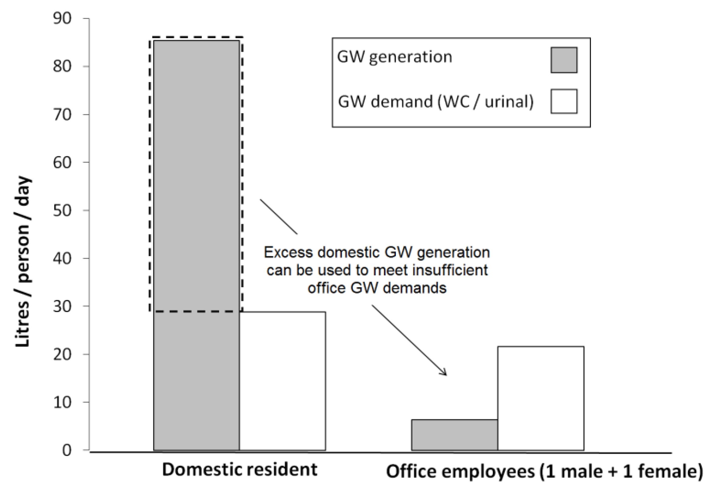
3/day) and costs £74,900 come from Scenario 1, where no GW collection or recycling occurs. The potable mains water demands are reduced by 19% in Scenario 2a and 2b, where GW is sourced from individual buildings. The related costs are reduced by 18%. However, whilst 27.8 m3/day of GW are collected, only 15.4 m3/day (55% of available supplies) of treated GW are needed. However, there is insufficient GW to meet demands in Offices in Scenario 2a and 2b. In contrast, the potable main water demands in Scenario 3a and 3b are reduced by 28% and costs are reduced by 29%. [In this case, the 23.3 m3/day demand for GW represents 94% of the available supply from domestic showers. Whilst this appears to be sufficient, it would likely not meet any additional system losses or significant fluctuations in demand encountered during the day. It is for this reason that GW is collected also from hand basins in residential blocks leading to a total supply of 28.9 m3/day (i.e., an oversupply of 24%).] Wastewater generation follows the same pattern as water demands, meaning that Scenario 1 has the highest outflow and Scenario 3a and 3b the lowest outflow.
Table 4. Flow rates and related cost savings across scenarios.
Various flows (units m3/day unless stated otherwise)Scenario
1 (Domestic, Office)2a2b3a3b
Potable mains water demand a 79.8 (63.9, 15.9)64.464.457.457.4
Domestic GW demand0.012.412.412.412.4
Office GW demand0.010.710.710.710.7
Domestic GW generation 0.024.924.928.928.9
Office GW generation 0.02.92.90.00.0
Total GW recycled and used0.015.415.423.123.1
Wastewater generation a 78.2 (62.6, 15.6)62.662.656.256.2
WTP and WTTP charges (£K/yr) b, c 74.9 (63.6, 11.3)61.261.253.353.3
Total savings (£K/yr)0.013.613.621.521.5
a Based on data from Table 1, Table 2 and Table 3; b assuming a price of £1.62 per m3 for potable water supply and £1.13 per m3 for sewerage charges (based on OFWAT (Office of Water Services, United Kingdom), 2011–2012 tariffs [48]); c assuming offices are in operation 261 days/yr and domestic flats are in operation 365 days/yr.

3.3. Expenses: CAPEX and OPEX

The total expenditure is a function of capital cost (CAPEX, Table 5), operational and maintenance costs (OPEX, Table 7) [29]. The various assumptions are shown in the tables, and where appropriate, a more detailed discussion follows.
In terms of CAPEX, the following assumptions were made:
The distance between buildings and the treatment plant determines the length of the greywater collection and distribution pipes and, thus, factors into the capital cost of system. The various pipework lengths are shown in Table 6. It was found that doubling and tripling the distance between buildings (200/300 m) and the treatment plant increases the CAPEX of system by 0.2% and 0.4%, respectively. A concrete tank with inner lining is selected: the tank size is specified to meet the total volume of daily GW demands (Table 4), plus an extra 10% to accommodate any losses in the treatment process (i.e., in VFCW to account for evapo-transpiration (losses of 15 l/m²/d) and in MBR to account for functions like filter backwash—where treated water is at regular intervals flushed back through the filter to help keep filters clean [43,47]. In each case, two tanks are adopted (one before and one after treatment); to level fluctuations in inflow and on the demand side. Filters are included to remove the solid particles, such as hair and skin from the raw greywater, before it enters the treatment systems, either MBR or VFCW; MBR consists of a compact unit, which combines activated sludge treatment for the removal of biodegradable pollutants and a membrane for solid/liquid separation [49]. MBR is commonly used in large buildings, such as multi-storey buildings [50,51,52], student accommodation [6], stadiums [50] and communal residential buildings [27]. GW treatment facilities are fed by gravity and pumping is only required for redistribution of treated GW. An MBR still requires a pump, but the energy demand is included in the energy demand value for MBR treatment (see Table 7). The pumps are designed based on the required daily flow in the system and total dynamic head (including operating head required by toilet fixtures), friction losses in the system and elevation difference between pump and the last fixture in the last floor based on the assumed buildings description. The CombiBloc centrifuge pump was selected based on the estimated required flow and total dynamic head from Johnsons Pump Company in the UK [53]. The main barrier is its high energy requirement (see later); VFCW replicates natural wetlands, improving water quality through physical, chemical and biological treatment mechanisms [54]. The main barriers to implementing constructed wetlands are the land requirement, scarce in urban areas, and the cost of the system increases proportionally to the land area required. Although, in the present study, the VFCW system was selected for GW treatment, because it requires less space (1 to 2 m2 per employee) than other constructed wetlands configurations, in addition, it offers a more appropriate and robust treatment within urban settings [55]. Both MBR and VFCW are not inappropriate to a UK setting [4,30,55,56]. The various sizes of VFCW are shown in Table 8. It can be seen that a much larger bed is required for Scenario 3b, as more GW volume is collected, treated and used. In Scenario 3, it can be seen that the CAPEX of the VFCW is much higher. This is because the economy of scale does not apply for this type of system, and the ratio between investment in the treatment system is proportional to the treated volume flow (even if in Scenario 2, two different units need to be constructed). For the MBR, the CAPEX for the treatment system drastically decreases from Scenario 2a to 3a, because in 3a, only one (larger) unit is required compared to two (smaller) units in 2a. However, the volume flow and, hence, the required membrane area in 3a is still bigger than in 2a.
Table 5. Generic CAPEX compared across scenarios.
Various costs (£K)Scenario
12a2b3a3b
Pipe work a,b- 14.515.411.812.5
Pump(s) c-0.310.290.310.31
Storage tank(s) d-2.82.83.13.1
Filter(s)-0.230.140.580.58
Installation e-1.01.01.01.0
Treatment system -65.8 f
Domestic = 41.2 (12.4 m3/d)
Office = 24.6 (2.96 m3/d)
44.2 g
Domestic = 33.8 (12.4 m3/d)
Office = 10.4 (2.96 m3/d)
49.2 f66.3 g
Total CAPEX -84.663.865.983.8
a Collection and distribution pipe sizes are based on author calculations—sizes range from 100 mm (inter-building connection) to 12.5 mm (internal connections within flats); b prices are based on PVC pipes supplied through UK manufactures in 2012; c CombiBloc (Pump Type 40-250) centrifugal pump (Johnsons pump company, 2012) [53]; d the storage tank is sized based on the greywater volume used per day in each scenario; prices for underground storage tank are adapted from Roebuck [43] and updated to 2012 using an average rate of inflation; e based on volume of greywater treated—the price includes purchase, delivery and installation from leading UK MBR manufacturers; f based on volume of treated greywater and effluent quality requirement—the price includes excavation, materials, and installation and is based on data from leading UK CW companies (Table 8), plus land purchasing prices in the Birmingham city centre area in the UK (£65/m2) and considering 1m2/PE [55].
Table 6. Various pipe sizes and lengths (in m) adopted in scenarios.
Pipe type (Diameter -mm)Scenario
12a2b3a3b
PVC (12.50)-10,324 10,3248,394 8,394
PVC (18.75)-390352--
PVC (25.00)-352352352983
PVC (31.25)-180350125175
PVC (50.00)-33843384
PVC (62.5)-97849784
PVC (100.0)-5858-82
Table 7. Annual OPEX compared across scenarios.
Various costs (£K)Scenario
12a2b3a3b
Water quality analysis a-1.381.380.690.69
Energy (distribution system) b, c-0.070.070.1440.144
Energy (treatment system) b, d-1.060.081.810.017
Equipment renewal (distribution system) e-0.0270.0270.0230.023
Equipment renewal (treatment system) f-0.4870.058 [17.7]0.2650.08 [26.6]
Consumable cost g-0.1600.7620.2431.239
Labour cost h-0.7532.6140.8243.556
Sludge disposal i-0.08-0.04-
Total OPEX-4.024.994.045.74
a One time per year for chemical analyses and one times per year for microbiological analyses at each system [57] (the price reduces by 50% after three years of system operation); b 13 Pence/KWh (average UK electricity charge from 2012) [58]; c based on CombiBloc (Pump type 40–250) centrifuge pump performance data [50] and assumes 12 hours of pump operation per day; d adopted form Nolde [48] and Freidler and Hadari [49] for MBR and from Dillon [59] and leading UK CW companies; e includes the cost for replacing the pumps every 10 years and filters every five years, plus considering 2% of capital costs per year for general repair costs for other distribution system [60,61]; f in scenarios with MBR (2a and 3a), membrane modules (three MBR modules for Scenarios 2a and five MBR modules for Scenario 3a) were replaced every two years [57]—there is no decisive criterion that triggers end of membrane life [62], and two years (730 days) is not inappropriate based on maintaining at least a 98% threshold from the original manufacturers permeability rating [63]. (N.B. Membranes can be, and are, used for longer, however, with a reduction in permeability performance, i.e., a 50% reduction is estimated by 3,400 days [63]). Price of each MBR modules is £200 (UK MBR manufacturers, 2012). In scenarios with CW (2b and 3b), the reeds in the bed requires harvesting and weeding, while the whole bed should be replaced with new material and plants every six years (depending on site condition and greywater quality); the italicised values in brackets indicate the costs on Year 6, when bed replacement is required for vertical flow constructed wetland (VFCW); g chemicals for membrane maintenance (NaOH (3kg/m3 of greywater treated) and NaOCl (0.67 kg/m3 of greywater treated)) and chemicals for greywater disinfection (0.003 kg of chlorine per m3 of greywater, [52]) in CW treatment; h routine inspection: two hours per week for general system, two times per year, for four hours with two persons for the MBR system and, for CW, includes weeding every two2 months for 10 minutes per m2 of bed, plus harvesting two times a year with 10 minutes per m2 of bed. Labour cost = 11.7 £/h [61]; i based on the price to empty 4 m3 of sludge every three years [56].
Table 8. Materials adopted in constructed wetland (CW) bed; volumes of each shown.
Bedding material (diameter, mm)Depth (m)Scenario
12a2b3a3b
Sand (0.5) 0–0.3--401 m3-602 m3
Gravel—fine (6)0.3–0.4--152 m3-229 m3
Gravel—medium (24.4)0.4–0.65--382 m3-573 m3
Cobbles—coarse (90.0)0.65–0.75--134 m3-201 m3
In terms of OPEX the following assumptions were made:
The energy requirements for distribution system were calculated using Equations 8 to 10. The respective parameters used therein are presented in 
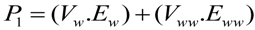
Table 4. In all scenarios, there is an energy requirement related to (pipeline) delivery of mains water and removal of wastewater, as shown in Equation 8:
Sustainability 05 02887 i001
Were Vw is the volume of potable water delivered (m3), Ew is the energy requirements per m3 of potable water delivered (0.73 kWh/m3), Vww is the volume of wastewater removed (m3) and Eww is the energy requirements per m3 of wastewater removed (0.19 kWh/m3) [
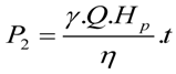
64]. The energy requirement for pumping water through the treatment process and from the final storage tank to point of end-use was estimated using Equation 9:
Sustainability 05 02887 i002
Where P2 is the energy delivered to the pump, Sustainability 05 02887 i003 is the specific weight of water (N/m3), Q is the flow rate (m3/s), η is the overall pump efficiency (i.e., mechanical and hydraulic), which is assumed to be 65% [65], t is the time interval for pump operation and H
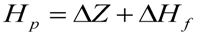
p is the required head to be supplied by the pump (m), as shown in Equation 10:
Sustainability 05 02887 i004
where ΔZ is the elevation difference (the maximum value is equal to the height of the top floor of the building plus the depth of buried pipe underground). ΔHf is the head lost in pipes due to friction and is estimated by using the Hazen-Williams equation [
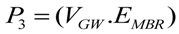
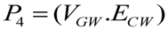
65]. The energy for treating GW via MBR and VFCW is calculated using Equation 11 and 12, respectively:
Sustainability 05 02887 i005
Sustainability 05 02887 i006
where VGW is the volume of GW treated (m3) and EMBR (1.5kWh/m3) [51,52,57] and ECW (0.014kWh/m3) [59] are the energy requirements for treating GW either through MBR or VFCW, respectively.
A design life of 15 years was assumed for both systems [26,49]. For example, replacement materials were assumed as follows: pumps were replaced after 10 years, filters every five years, membranes for MBR after two years [57] and the bed and plant for VFCW are rebuilt after six years.

3.4. NPV

Net Present Value (NPV) is the present value of an investment’s future net cash flows minus the capital investment (Equation 13). It is one of the most commonly used tools for comparing the amount invested today to the present value of the future cash receipts from the investment [66,67] customary to invest in projects with positive NPV:
Sustainability 05 02887 i007
where:
  • r = economic discount rate (%),
  • l = life of the project (taken as 15 years), and
  • Cn = cash flow of evaluated scenario (i.e., savings and expenditure) minus the cash flow of Scenario 1 for year, n.
In all five scenarios, a 15-year lifetime (consistent with the design life), 4% discount rate [68], current average Birmingham price of water and wastewater (assumed to increase at 8.5%per annum) and typical water micro-components inside buildings were used for analyses.

4. Results and Discussion

In this section, the results of the initial NPV analysis are presented (Section 4.1). In the proceeding sensitivity analyses, this is then referred to as the ‘base’ case. By making changes to annual changes in water and wastewater charges (4.2.1), discount rates (4.2.2), service life (4.2.3) and technological efficiency of micro-components (4.2.4), a sensitivity analysis of NPV in each scenario was considered. (The effect of altering the user behaviour and occupancy rates were not considered in this study.) The NPV of each scenario is calculated with respect to the cash flows of Scenario 1. This comparison provides a measure of the cost effectiveness for each Scenario.

4.1. Initial NPV Analysis: 15 Year Operation

Figure 7 shows the NPV for all six Scenarios when considering 15 years of operation, from where it can be seen that there is a higher (positive) NPV for shared GW systems. This is due to higher savings related to potable main water supply and wastewater discharge, as compared to individual GW systems. The highest NPV belongs to Scenario 3a (a shared GW recycling system with MBR treatment). The NPV for Scenario 3b (a shared GW recycling system with VFCW treatment) is almost 30% lower than Scenario 3a, although still positive in value. A comparison between the two treatment options shows that the overall OPEX of a VFCW is higher than the MBR treatment system, mainly because labour and consumable cost compensate for the low energy requirements of the VFCW (Table 6); the CAPEX for a shared VFCW is also much higher (Table 5a). This is because the economy of scales does not apply for this type of system; in other words, the costs of site mobilisation and demobilisation (i.e., to get the contractor to start allocated works and, ultimately, clear the site) would be the same independent of the size of the system adopted. In countries with lower labour cost or using different sterilisation method, other conclusions may, hence, be reached. Whilst Scenario 2b does show a positive NPV for individual domestic systems, there is a negative NPV for individual office systems; however, the cumulative NPV is positive. In Scenario 2a, the influential factor is the negative NPV value for offices. In all cases, it can be seen that a cumulative positive NPV can be achieved (i.e., NPV for offices and domestic added together). In other words, money would be saved as compared to Scenario 1 (the ‘main only’ scenario).
Figure 7. Total cost of scenarios for a typical residential and office building over a 15-year lifetime (from here onwards, this is referred to as ‘base’).
Sustainability 05 02887 g007

4.2. NPV Sensitivity Analyses

4.2.1. Sensitivity Analysis 1: Annual Changes in Water Supply and Wastewater Charges

In this analysis, it is assumed that the unit costs (£/m3) for water supply and sewage removal (excluding standing charges) increases at an annual rate of between 0 to 10%. It is worth noting that the suggested price cap from the UK water industry of 50% by 2015 (compared to 2010 prices) would lead to an annual growth rate of 8.5%, not dissimilar to the growth rate used in the base case [4]. The impact of this range of annual increases can be seen in Figure 8a. The resulting graph displays a positive gradient, indicating that as charges are increased, the cost effectiveness of the GW recycling system for each scenario also increases.

4.2.2. Sensitivity Analysis 2: Discount Rates

In this analysis, it is assumed that discount rates could range from 0% to 15%. In Figure 8b, it can be seen that any change to discount rate compared to the ‘base’ case results in an exponential decay relationship with cost effectiveness of GW recycling systems. As the discount rate approaches 15%, the NPV of Scenario 2a passes through zero (point A).
Figure 8. Sensitivity results of NPV to (a) changes in main water and wastewater charges, (b) discount rate and (c) service life.
Sustainability 05 02887 g008

4.2.3. Sensitivity Analysis 3: Service Life

In this analysis, the impact of service life (5 to 20 years) on financial feasibility of scenarios is considered. It can be seen from Figure 8c that longer discount periods compared to the ‘Base’ case lead to an increase in the NPV for each scenario. This general trend supports the fact that a longer service life will result in more income generated from water and wastewater savings, which, in turn, covers more of the capital cost of systems. Likewise, when service life is reduced to five years (or less), the NPV for all scenarios (excepting scenario 3a) becomes negative, due to insufficient accumulation of savings (from water and wastewater) to offset expenses (point B). Subsequently, an increase in service life to 20 years results in significantly greater value of NPV for all scenarios. In addition, the NPV for Scenarios 2a and 2b become positive (with transitions at 6 and 7 yrs, respectively), with values being broadly similar (point C). This was likely due to the costs being dominated by maintenance requirements (OPEX) for VFCW treatment in Scenario 2b.

4.2.4. Sensitivity Analysis 4: Technological Efficiency

In this analysis, the impact on NPV of changing water efficient appliances (technology) within each building is considered. By changing the technology efficiency in this way, whilst keeping other variables constant (e.g., water charges or discount rate), provides a direct measure of their impact on the economic performance of shared and individual GW recycling systems. A set of five design cases for domestic demands (Table 9) in the UK has been derived using the water efficiency calculator for new dwellings [8,37]. The five design cases for office demands (Table 10) have been derived based on Waggett and Arotsky [23], Hunt et al. [8] and BREEAM (British Research Establishment Environmental Assessment Method) for offices [39].
Table 9. Domestic technological efficiency by end-use for each design case.
Technology (units)Design case
(D1)(D2)(D3)(D4)(D5)
WC (lit/flush)a664.54 .52.5
Washing Machine (lit/load)11080494935
Lavatory taps (lit/min)128655
Kitchen taps (lit/min)128655
Shower (lit/min)15121086
Bath (lit/usage)2301161168865
Dishwasher (lit/load)2525161414
a For more information on the effects of low flush toilets on GW systems and wider infrastructure systems, see [69,70].
Table 10. Office technological efficiency by end-use for each design case.
Technology (units)Design Case
(O1)(O2)(O3)(O4)(O5)
WC (lit/flush)664.522
Urinal (lit/bowl/hr)7.57.53.53.51.5
Lavatory taps (lit/min)128664
Kitchen taps (lit/min)128664
In order to calculate the volume of water used by each resident/employee, the chosen technological efficiency parameter is multiplied by a factor related to user behaviour (Table 2, Table 3). It is important to note that user behaviour has a direct impact on the amount of potable water used throughout homes, and it is assumed to remain unchanged within all the design cases.
The total water in each design case (residential and office buildings) is shown in Table 11. Domestic design case, D2, and office design case, O2 (shown in bold), represent the base case. The ‘cleaning routine’ and ‘canteens use’ (Table 3) in offices and ‘other uses’ in domestics (Table 2), not shown in these tables, were assumed to be constant in all design cases. The resulting changes to NPV (compared to the ‘base’ case), according to variations in technological efficiency within domestic and office buildings, are shown in Figure 9a,b, respectively.
Table 11. Total water consumption for each Domestic (D) and Office (O) design case. (italics shows where female water usage differs).
Water consumptionDesign Case
(D1)(D2)(D3)(D4)(D5)
Total (lit/capita/day)19614811810176
Water consumptionDesign Case
(O1)(O2)(O3)(O4)(O5)
Total (lit/capita/day)16.7 (21.8)15 (19.4)10.5 (14.8)7.6 (9.1)5.7 (7.9)
Figure 9. (a) Influence of residential technology changes on NPV; (b) influence of office technology changes on NPV.
Sustainability 05 02887 g009

5. Conclusions

This study compares the total costs of individual and shared GW recycling systems, using two different treatment technologies (MBR and VFCW). Five scenarios were analysed for residential and office buildings specifically chosen to be representative of UK urban mixed-use regeneration areas. Economic analyses were conducted using NPV calculations, and a sensitivity analysis was employed to determine the impact of changes to costs of water and wastewater, discount rates, service lifetime and technological efficiency.
In conclusion, the NPV of MBR water treatment was greater than NPV of VFCW water treatment for shared systems. Moreover, the NPV achievable through the adoption of shared systems was greater than for individual systems. The analyses showed that larger GW systems with MBR treatment have a higher NPV, because of economy of scales in MBR, which cannot be achieved for VFCW. The major cost driver in CW is the land price, and as the focus of this study was on urban areas, the land prices are considerably high, which makes this treatment technology less favourable than others. Subsequent studies might wish to look under which circumstances the CW technology is more beneficial by considering the influence of lower land pricing in addition to labour costs, less expensive filling materials and a range of treatment units (with alternatives to chlorine).
In all cases, the improvement in technological efficiency reduced the value of NPV, this impact being more noticeable in domestic buildings than offices. In individual GW recycling systems, the water saving potential for homes is limited by demand and not supply. In offices, the added inconvenience is low volumes (i.e., low absolute savings); moreover, it is independent of technology type. Shared GW recycling systems (MBR) resulted in the highest (positive) NPV and highest water saving potential (28%, with no change to technological efficiency).
GW recycling is not yet widely accepted in practice, partly because of the low economic benefit, particularly in commercial buildings, such as offices. The findings from this paper show that a shared GW recycling system can carry lower economic costs in both high and low efficiency buildings. The same methodology can be extended within the UK to buildings with different uses, including hotels, educational facilities, commercial premises and malls. In addition, it is applicable to country-specific patterns of water use. As the cost of water rises and increasing pressure is placed upon aging and deteriorating water and wastewater infrastructure, solutions that reduce water demand, such as greater use of greywater, become more viable financially. Given that the utility service infrastructure created to support buildings typically has a design life of 20–40 years, adoption of systems that might be marginally more expensive now, but deliver considerable benefits in the future, should be seriously considered: possibly proving an immediate ‘selling point’ for the development and a future means to avoid retrofitting costs.

Acknowledgments

This study was funded by EPSRC under the current Liveable Cities Programme Grant (EP/J017698) and previous Sustainable Urban Environments Urban Futures grant (EP/F007426/1) and by the University of Birmingham via a post-graduate teaching assistantship to SMZ. The authors wish to thank the CW companies for providing information on the capital and operation costs of constructed wetlands in the UK. The authors wish also to thank the reviewers for the time spent reviewing this paper, which has helped strengthen it significantly. Full details of all of the analyses presented here can be found in Zadeh, 2013 [71].

Conflict of Interest

The authors declare no conflict of interest.

References

  1. World Water Assessment Programme. The United Nations World Water Development Report 3: Water in a Changing. Available online: http://www.unesco.org/water/wwap (accessed on 29 November 2009).
  2. International Water Management Institute (IWMI). Available online: http://www.iwmi.cgiar.org/ Publications/index.aspx (accessed on 14 September 2010).
  3. The Stationery Office (TSO), Water for life. Available online: http://www.official-documents.gov.uk/document/cm82/8230/8230.pdf (accessed on 9 August 2011).
  4. Environment Agency, The Case for Change: Current and Future Water Availability; Report GEHO1111BVEP-E-E. Environment Agency: Bristol, UK, 2012; p. 41.
  5. Environment Agency, The Case for Change: Reforming Water Abstraction Management in England; Report GEHO1111BVEQ-E-E; Environment Agency: Bristol, UK, 2012; p. 32.
  6. Surendran, S.S. The development of an in-house greywater and roof water reclamation system for large institutions, during 1994 to 1998. PhD thesis, Department of Civil and Building Engineering, Loughborough University, UK, 2000. [Google Scholar]
  7. Hunt, D.V.L.; Jefferson, I.; Lombardi, D.R. Sustainable water supplies. A feasibility study for Birmingham Eastside. Eastside development. Available online: http://www.eastsidebirmingham.co.uk/ (accessed on 10 November 2009).
  8. Hunt, D.V.L.; Lombardi, D.R.; Farmani, F.; Jefferson, I.; Memon, F.A.; Butler, D.; Rogers, C.D.F. Urban Futures and the code for sustainable homes. Inst. Civ. Eng. Eng. Sustain. 2012, 165, 37–58. [Google Scholar]
  9. Zadeh, S.M.; Lombardi, D.R.; Hunt, D.V.L.; Rogers, C.D.F. Local area greywater symbiosis approach to a more sustainable urban water management. WIT Trans. Ecol. Environ. 2010, 142, 193–203. [Google Scholar]
  10. Tjandraatmadja, G.; Sharma, A.K.; Grant, T.; Pamminger, F. A decision support methodology for integrated urban water management in remote settlements. Water Resour. Manag. 2012, 27, 433–449. [Google Scholar] [CrossRef]
  11. Mandal, D.; Labhasetwar, P.; Dhone, S.; Dubey, A.S.; Shinde, G.; Water, S. Water conservation due to greywater treatment and reuse in urban setting with specific context to developing countries. Resour. Conserv. Recycl. 2011, 55, 356–361. [Google Scholar] [CrossRef]
  12. Jefferson, B.; Palmer, A.; Jeffery, P.; Stuetz, R.; Judd, S. Greywater characterisation and its impact on the selection and operation of technologies for urban reuse. Water Sci. Technol. 2004, 50, 157–164. [Google Scholar]
  13. Santala, E.; Uotila, J.; Zaitsev, G.; Alasiurua, R.; Tikka, R.; Tengvall, J. Microbiological greywater treatment and recycling in an apartment building. In Proceedings of the 2nd International Advanced Wastewater Treatment, Milan, Italy, 14–16 September 1998; pp. 319–324.
  14. Surrendran, S.; Wheatley, A. Grey water reclamation for non-potable re-use. J. CIWEM 1998, 12, 406–413. [Google Scholar]
  15. Brewer, D.; Brown, R.; Stanfield, G. Rainwater and Greywater in Buildings: Project Report and Case Studies; Report 13285/1; BSRIA Ltd.: Bracknell, UK, 2000. [Google Scholar]
  16. March, J.; Gual, M.; Orozco, F. Experience on greywater reuse for toilet flushing in hotel (Mallorca Island, Spain). J. Desalination 2004, 164, 241–247. [Google Scholar] [CrossRef]
  17. Leggett, D.; Brown, R.; Brewer, D.; Stanfield, G.; Holliday, E. Rainwater and Greywater Use in Buildings. Best Practice Guidance; CIRIA publications, C539; Construction Industry Research and Information Association (CIRIA): London, UK, 2001. [Google Scholar]
  18. Day, M. The Millennium Green Development Rainwater Project. In Proceedings of 22nd meeting of the Standing Conference on Stormwater Source Control: Quantity and Quality, Coventry University, UK, 13 February 2002.
  19. Hills, S.; Birks, R.; McKenzie, B. The Millennium Dome “Watercycle” experiment: To evaluate water efficiency and customer perception at a recycling scheme for 6 million visitors. Water Sci. Technol. 2002, 46, 233–240. [Google Scholar]
  20. Bray, R. The Operation and Maintenance of Sustainable Drainage Systems (and Associated Costs)—A Review of the DTI Report SR626. In Proceedings of the 3rd National Conference on Sustainable Drainage, Coventry University, UK, 20–21 June 2005; pp. 102–114.
  21. Coombes, P.J.; Boubli, D.; Argue, J.R. Integrated Water Cycle Management at the Heritage Mews Development in Western Sydney. In Proceedings of 28th International Hydrology and Water Resources Symposium, Wollongong, Australia, 10–14 November 2003.
  22. Loh, M.; Coghlan, P. Domestic Water Use Study in Perth, Western Australia 1998–2001; Water Corporation: Perth, Australia, 2003. [Google Scholar]
  23. Paul, I.; Bray, R. SUDS in a School Context. In Proceedings of 25th meeting of the Standing Conference on Stormwater Source Control: Quantity and Quality, Coventry University, UK, 20 February 2004.
  24. CIWEM. The Chartered Institution of Water and Environmental Management website. Available online: http://www.ciwem.org/resources/water/rainwater/edenproject.asp (accessed On 15 October 2009).
  25. Mourad, K.A.; Berndtsson, J.C.; Berndtsson, R. Potential fresh water saving using greywater in toilet flushing in Syria. J. Environ. Manag. 2011, 92, 2447–2453. [Google Scholar] [CrossRef]
  26. Waggett, R.; Arotsky, C. Water Key Performance Indicators and Benchmarks for Offices and Hotels; CIRIA publications, C657; Construction Industry Research and Information Association (CIRIA): London, UK, 2006. [Google Scholar]
  27. Lazarova, V.; Hills, S.; Birks, R. Using recycled water for non-potable, urban uses; a review with particular reference to toilet flushing. Water Sci. Technol. 2003, 3, 69–77. [Google Scholar]
  28. Leggett, D.J.; Shaffer, P. Buildings that save water–rainwater and greywater use. Proc. Inst. Civ. Eng. (Municipal) 2002, 151, 189–196. [Google Scholar]
  29. Memon, F.A.; Butler, D.; Han, W.; Liu, S.; Makropoulos, C.; Avery, L.; Pidou, M. Economic assessment tool for greywater recycling systems. Proc. Inst. Civ. Eng. Eng. Sustain. 2005, 158, 155–161. [Google Scholar]
  30. Pidou, M.; Memon, F.A.; Stephenson, T.; Jefferson, B.; Jeffery, P. Greywater recycling: Treatment option and applications. Inst. Civ. Eng. Proc. Eng. Sustain. 2007, 160, 119–131. [Google Scholar]
  31. Building Regulation (2011). Effects of recent and Future changes. Available online: http://www.theapprovedinspector.com/CIOB%202011.pdf (accessed on 19 May 2012).
  32. Diaper, C.; Jefferson, B.; Parson, S.; Judd, S. Water recycling Technologies in the UK. Water Environ. J. 2001, 15, 282–286. [Google Scholar] [CrossRef]
  33. LHDG (London Housing Design Guide). Available online: http://www.designforlondon.gov.uk/ uploads/media/Interim_London_Housing_Design_Guide. pdf (accessed on 19 April 2012).
  34. Market Transformation Programme. Domestic water consumption in domestic and non-domestic properties. Available online: http://www.mtprog.com/ApprovedBriefingNotes/PDF/MTP_BNWAT22_2008March28.pdf (accessed on 19 April 2012).
  35. Porter, E.J.; Hunt, D.V.L. Eastside: Making steps towards sustainability? Local Environ. Taylor Francis Group 2005, 10, 525–542. [Google Scholar] [CrossRef]
  36. Hunt, D.V.L.; Lombardi, D.R.; Rogers, C.D.F.; Jefferson, I. Application of sustainability indicators in decision-making processes for urban regeneration projects. Eng. Sustain. Proc. Inst. Civ. Eng. 2008, 161, 77–91. [Google Scholar]
  37. SODCON. The annual Survey of Domestic Consumption. Available online: http://www.anglianwater.co.uk/environment/water-resources/02380F3AEA7B42C3A68126D2A0108B82.aspx (Accessed 21 April 2012).
  38. Butler, D. The influence of dwelling occupancy and day of the week on domestic appliance wastewater discharges. Build. Environ. 1991, 28, 73–79. [Google Scholar] [CrossRef]
  39. Chambers, V.K.; Creasey, J.D.; Glennie, E.B.; Kowalski, M.; Marshallsay, D. Increasing the Value of Domestic Water Use Data for Demand Management–Summary Report; WRc collaborative project CP187, Report no. P6805; WRc: Swindon, UK, 2005. [Google Scholar]
  40. DCLG, Code for Sustainable Homes: Technical Guide; Department of Communities and Local Government, HMSO: London, UK, 2010.
  41. Environment Agency, Energy and Carbon Implications of Rainwater Harvesting and Greywater Recycling, Environment Agency: Bristol, UK, 2011.
  42. BREEAM. British Research Establishment Environmental Assessment Method. Available online: http://www.breeam.org/about.jsp?id=66 (accessed on 12 October 2011).
  43. Roebuck, R.M. A whole life costing approach for rainwater harvesting systems. PhD thesis, University of Bradford, Bradford, UK, 2007. [Google Scholar]
  44. Hills, S.; Smith, A.; Hardy, P.; Birks, R. Water recycling at the Millennium Dome. Water Sci. Technol. 2001, 43, 287–294. [Google Scholar]
  45. Water Regulations Advisory Service (WRAS). Reclaimed Water Systems: Information about installing, modifying or maintaining reclaimed water systems. 1999. Available online: http://www.wras.co.uk/pdf_files/IGN%209-02-04%20Reclaimed.pdf (accessed on 20 April 2012).
  46. Ghisi, E.; Oliveria, M.S. Potential for potable water savings by combining the use of rainwater and greywater in houses in southern Brazil. Build. Environ. 2007, 42, 1731–1742. [Google Scholar] [CrossRef]
  47. MJA, The cost-effectiveness of rainwater tanks in urban Australia; Report prepared by Marsden Jacob Associates for the National Water Commission; National Water Comission: Canbera, Australia, 2007.
  48. Charges and bills publications 2011-12. Available online: http://www.ofwat.gov.uk/regulating/ charges/prs_web_charges2011-12 (accessed on 25 March 2012).
  49. Memon, F.A.; Zheng, A.; Butler, D.; Shirley–Smith, C. Life cycle impact assessment of greywater recycling technologies for new developments. J. Environ. Monit. Assess. 2007, 129, 27–35. [Google Scholar] [CrossRef]
  50. Merz, C.; Scheumann, R.; El Hamouri, B.; Kraume, M. Membrane bioreactor technology for the treatment of greywater from a sports and leisure club. Desalination 2007, 251, 37–43. [Google Scholar]
  51. Nolde, E. Greywater reuse systems for toilet flushing in multi-story buildings- over ten years experience in Berlin. Urban Water 1999, 1, 275–284. [Google Scholar] [CrossRef]
  52. Friedler, E.; Hadari, M. Economic feasibility of on-site greywater reuse in multi-storey buildings. Desalination 2006, 190, 221–234. [Google Scholar] [CrossRef]
  53. Johnson Pump Company. Available online: http://www.spx.com/en/johnson-pump/ (accessed on 4 February 2012).
  54. USEPA Manual: Constructed Wetlands Treatment of Municipal Wastewater (EPA-625-R-99-010); US Environmental Protection Agency, Office of Research and Development: Cincinnati, OH, USA, 1999.
  55. Frazer-Williams, R.A.D. Constructed wetlands for advanced treatment and reuse. PhD thesis, University of Cranfield, Cranfield, UK, 2007. [Google Scholar]
  56. Li, F.; Wichmann, K.; Otterpohl, R. Evaluation of appropriate technologies for greywater treatments and reuses. Water Sci. Technol. 2009, 59, 249–260. [Google Scholar] [CrossRef]
  57. Mercoiret, L. Operating cost model for a neighbourhood grey water recycling scheme, unpublished. MSc Thesis, Cranfield University, Cranfield, UK, 2008. [Google Scholar]
  58. DECC, Department of Energy and Climate Change GHG conversion Factors for company reporting. DEFRA- Department for Environment Food and Rural Affairs: London, 2011. Available online: http://archive.defra.gov.uk/environment/business/reporting/pdf/110819-guidelines-ghg-conversion-factors.pdf (accessed 19 April 2012).
  59. Dillon, P. Banking of Stormwater, Reclaimed Water and Potable Water in Aquifers. In Proceedings of the international groundwater conference on sustainable development and management of groundwater resources in semi-arid region with special reference to hard rocks, Dindigul, Tamil Nadu, India, 20–22 February 2002; pp. 71–80.
  60. Asano, T. Wastewater Reclamation and Reuse; Water Quality Management Library, Technomic Publishing: Lancaster, PA, USA, 1998. [Google Scholar]
  61. SPONS, Civil Engineering and Highway Works Price Book, 25th ed; Taylor and Francis Ltd.: London, UK, 2011.
  62. Ayala, D.F.; Ferre, V.; Judd, S.J. Membrane life estimation in full-scale immersed membrane bioreactors. J. Membr. Sci. 2011, 378, 95–100. [Google Scholar] [CrossRef] [Green Version]
  63. Fenu, A.; de Wilde, W.; Gawrtner, M.; Weemaes, M.; de Gueldre, G.; van de Steene, B. Elaborating the membrane life concept in a full scale hollow-fibers MBR. J. Membr. Sci. 2012, 421, 349–354. [Google Scholar]
  64. Water UK. Sustainability indicators 2009/2010. London, UK, 2010. Available online: http://www.water.org.uk/home/news/press-releases/indicators2009-10/water-uk---sustainability-report-2009-10.pdf (accessed on 19 April 2012).
  65. Cengel, Y.; Cimbala, J. Fluid Mechanics: Fundamental and Applications; McGraw Hill Higher Education: Boston, MA, USA, 2005. [Google Scholar]
  66. Kirk, S.J.; Dell’Isola, A.J. Life Cycle Costing for Design Professionals; McGraw-Hill: New York, NY, USA, 1995. [Google Scholar]
  67. Swamee, P.K.; Sharma, A.K. Net Present Value or Present Value Method. In Design of Water Supply Pipe Networks, 4.3.3; Wiley Interscience: Hoboken, NJ, USA, 2008; pp. 110–111. [Google Scholar]
  68. HM Treasury, Basis for setting the discount rate for calculating cash equivalent transfer values payable by public service pension schemes, 2010. Guidance issued by HM Treasury. Available online: http://www.hm-treasury.gov.uk/ (accessed on 15 February 2011).
  69. Mourad, K.A.A.; Berndtsson, J.C.A.; Berndtsson, R.B. Potential fresh water saving using greywater in toilet flushing in Syria. J. Environ. Manag. 2010, 92, 2447–2453. [Google Scholar]
  70. Penn, R.; Schütze, M.; Friedler, E. Modelling the effects of on-site greywater reuse and low flush toilets on municipal sewer systems. J. Environ. Manag. 2013, 114, 72–83. [Google Scholar] [CrossRef]
  71. Zadeh, S.D. Sustainability Evaluation of shared greywater recycling in mixed-use regeneration areas. PhD thesis, Department of Civil Engineering, Birmingham University, UK, 2013. [Google Scholar]

