Economic Growth Assumptions in Climate and Energy Policy

Abstract

The assumption that the economic growth seen in recent decades will continue has dominated the discussion of future greenhouse gas emissions and the mitigation of and adaptation to climate change. Given that long-term economic growth is uncertain, the impacts of a wide range of growth trajectories should be considered. In particular, slower economic growth would imply that future generations will be relatively less able to invest in emissions controls or adapt to the detrimental impacts of climate change. Taking into consideration the possibility of economic slowdown therefore heightens the urgency of reducing greenhouse gas emissions now by moving to renewable energy sources, even if this incurs short-term economic cost. I quantify this counterintuitive impact of economic growth assumptions on present-day policy decisions in a simple global economy-climate model (Dynamic Integrated model of Climate and the Economy (DICE)). In DICE, slow future growth increases the economically optimal present-day carbon tax rate and the utility of taxing carbon emissions, although the magnitude of the increase is sensitive to model parameters, including the rate of social time preference and the elasticity of the marginal utility of consumption. Future scenario development should specifically include low-growth scenarios, and the possibility of low-growth economic trajectories should be taken into account in climate policy analyses.

1. Introduction

“Prediction is very difficult, especially about the future.” Niels Bohr’s caution would surely apply to extrapolating long-term change in the size and composition of the economic system, as technical innovation and changing values and social structures are likely to change the controlling forces at least as much as they have changed in recent centuries. Nevertheless, scenarios of future global economic growth and social change over century timescales are used in climate policy discussion for developing baseline emissions scenarios, evaluating the effects of different emissions-reduction policies and quantifying the harms to future generations of human-induced global warming. While diverse scenarios for economic growth, derived under different assumptions, have been used for different climate policy studies, they largely have in common that they assume a continuation of the rapid economic growth seen in the past century. Under these scenarios, per capita wealth a century or two in the future will be much greater than it is now.

Taking into account the possibility of economic growth rates at the lower end of the range of published scenarios and of historical experience, however, can substantially change perspectives on the capabilities for adapting to climate change and the wisdom of investment in mitigating greenhouse gas emissions. Broadly speaking, slower than anticipated economic growth would mean lower than expected demand for energy, which may result in reduced emissions compared with rapid-growth scenarios. However, in a relatively poorer society, large-scale investment in reducing the greenhouse gas intensity of energy consumption would be less feasible, and without sufficient development of renewable energy generation, distribution and storage, the energy supply may remain tied to highly polluting fossil fuels, such as coal and tar sands. The damage of climate impacts from greenhouse gas emissions and the cost of their mitigation would also be less manageable under slow economic growth than in a very wealthy society. Using a simple economic model of the cost of climate change to estimate optimal emissions control trajectories, substantially more aggressive actions to reduce carbon emissions now are justified if we assume slow economic growth in the coming centuries compared with scenarios assuming rapid economic growth.

This paper is organized as follows: First, I review the different socioeconomic scenarios used for climate research, placing emphasis on the 21st century gross world product (GWP) growth rate as a simple indicator of the economic growth trajectory assumed. Second, I qualitatively discuss possible implications of slow economic growth for greenhouse gas emissions trajectories and climate impacts. Third, I quantify the dependence of optimal present policy on assumptions about future economic growth in a simple integrated assessment model as an illustration of the qualitative considerations adduced. The overall goal is to explore the implications of low growth for climate policy in a risk assessment framework.

2. Assumptions about Economic Growth in the Climate Policy Literature

The Intergovernmental Panel for Climate Change (IPCC) has prepared several scenarios for the evolution of population, economic activity, energy use and greenhouse gas and sulfur emissions through 2100. The IPCC scenario sets are intended, and are widely used, to provide a range of illustrative greenhouse gas emissions series to drive climate models and to consider needs and options for the mitigation of and adaptation to climate change. 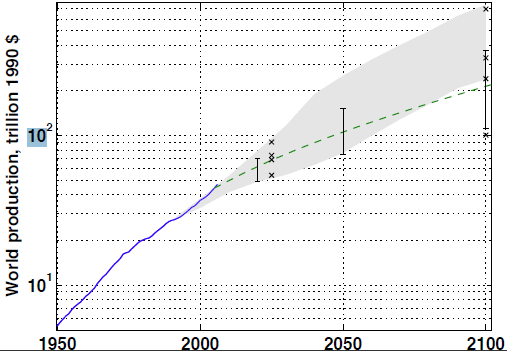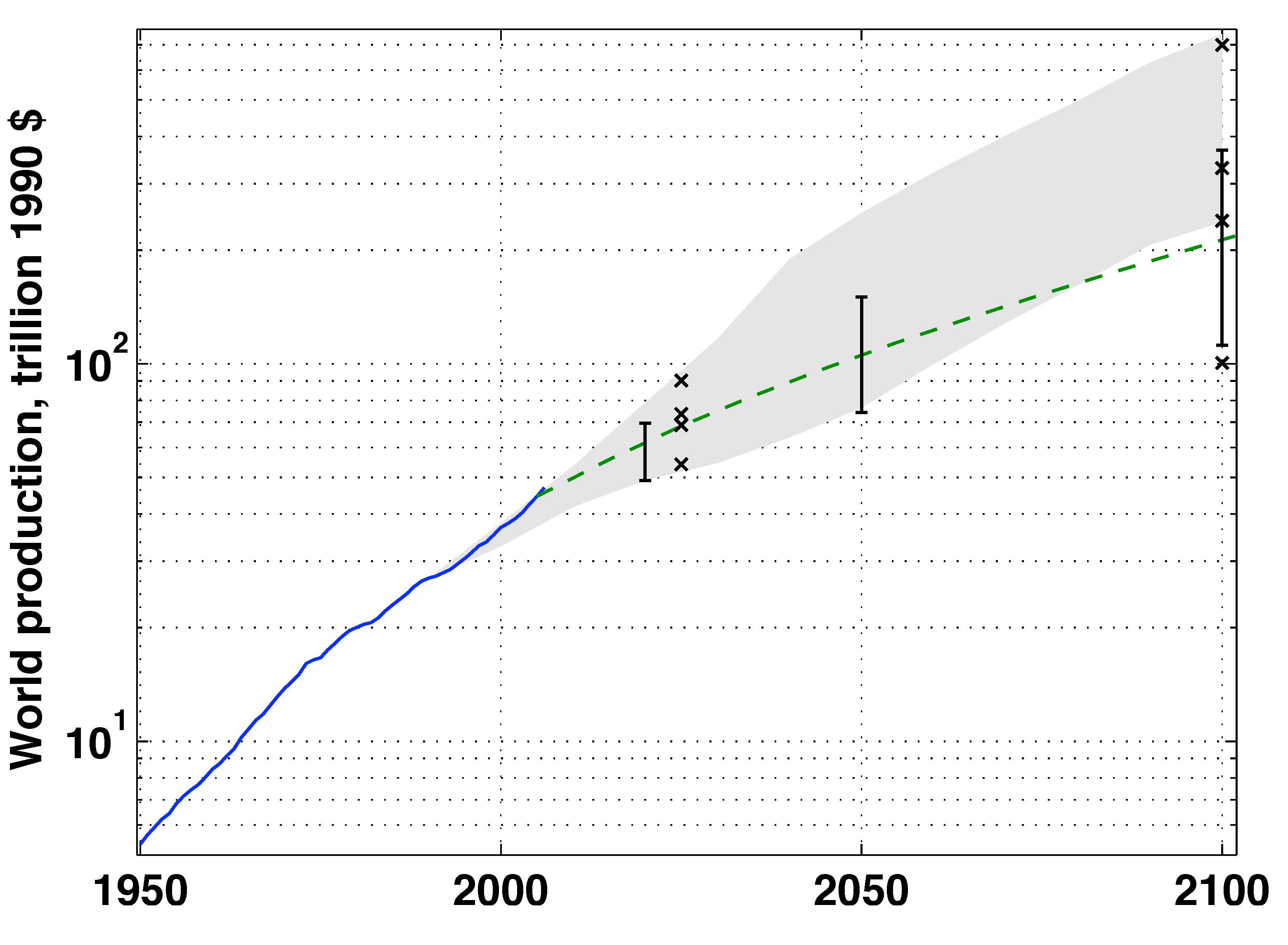Like an earlier IPCC scenario set released in 1992 [1], the IPCC’s Special Report on Emissions Scenarios (SRES) [2], released in 2000, envisions a wide range of possible worlds for 2100, encompassing 40 scenarios grouped into four “families” and six “groups”. In all the SRES scenarios, however, world economic production is much increased from the scenarios’ start year of 1990. From US$27 trillion in 1990, the annual gross world product (GWP) is taken to increase, in real terms, 9–28 fold (to $238–748 trillion, when the dollar amounts are scaled to a common value in 1990) by 2100 in the various SRES scenarios, corresponding to a rate of increase of 2.0%–3.1%/year over the 110-year period (Figure 1). Using the respective scenarios’ population projections, per capita GWP at 2100 would then be $16–106 thousand (1990 US dollars), up from $5 thousand in 1990. Even the lowest figure of $16 thousand is approximately equal to the 1990 per capita gross domestic product (GDP) of Italy or the United Kingdom and close to that of the wealthiest countries in 1990 (the United States and Luxemburg, with per capita GDP of some $23 thousand) [3]. Thus, even the most conservative SRES scenario envisions that economic growth will be sufficient to provide each of the 7–15 billion people assumed to live in 2100 with a standard of living comparable to that now common only in a relatively few wealthy countries (although, depending on wealth distribution, many people might still be poor). Interestingly, the range of 2100 GWP is narrower in SRES than in the earlier, less extensively documented 1992 IPCC scenario set, which features six scenarios (referred to as the 1992 IPCC scenario (IS92) set) that have a range of growth rates in 1990–2100 of 1.2%–3.0%/year, corresponding to 2100 GWP ranging from approximately $100 trillion (for scenario IS92c) to $700 trillion (for scenario IS92e) (Figure 1).

Figure 1. Scenarios of future growth in world production. Shown are historic production growth for 1950–2006 (solid line), the range of projected production (fifth to 95th percentile) for 2050 and 2100 among the scenarios collected in the Intergovernmental Panel for Climate Change (IPCC) database (error bars), production in the four distinct 1992 IPCC economic scenarios for 2025 and 2100 (x markers), the range of production in Special Report on Emissions Scenarios (SRES) scenarios for 1990–2100 (gray shading) and the growth trajectory of the DICE-2007 integrated assessment model with default parameter values (dashed line). The vertical scale is logarithmic, so that a constant growth rate would plot as a straight line.

Figure 1. Scenarios of future growth in world production. Shown are historic production growth for 1950–2006 (solid line), the range of projected production (fifth to 95th percentile) for 2050 and 2100 among the scenarios collected in the Intergovernmental Panel for Climate Change (IPCC) database (error bars), production in the four distinct 1992 IPCC economic scenarios for 2025 and 2100 (x markers), the range of production in Special Report on Emissions Scenarios (SRES) scenarios for 1990–2100 (gray shading) and the growth trajectory of the DICE-2007 integrated assessment model with default parameter values (dashed line). The vertical scale is logarithmic, so that a constant growth rate would plot as a straight line.

Broadly similar economic growth assumptions have been adopted even in studies of the economic impact of global warming and of alternative mitigation strategies that do not employ IPCC scenario sets. The assumptions about economic growth in William Nordhaus’ work with the Dynamic Integrated model of Climate and the Economy (DICE) model [4,5,6] result in 21st-century growth trajectories just below the lower bound of the SRES envelope. The model version DICE-2007 averages 1.6%/year growth in world product (1.4%/year growth in per capita world product) over the period 2005–2100, for per capita GWP of US$27 thousand (1990 dollars) in 2100. The Stern Review of the economics of climate change [7] uses a different model, Policy Analysis for the Greenhouse Effect (PAGE2002), which similarly averages 1.3%/year growth in per capita output for 2001–2200, a rate which, for the purpose of calculating the present value of future climate-change damage, is extended into the indefinite future. Earlier studies that sought to estimate future emissions changes (e.g., [8,9,10]) or consider the merits of alternative emissions abatement strategies (e.g., [11]) have also assumed that per capita GWP will increase by 1%–2%/year at least through 2100.

The assumption of steadily increasing production is usually justified by extrapolation from recent (19th and 20th century) production growth, as observed globally or in particular groups of countries [8,9,11,12]. Often, there is an appeal to the consensus of earlier scenarios. The most extensive work here has been done by SRES, which complied a database of over 100 long-term climate scenarios and writes about the histogram of economic growth in these scenarios: “A very strong peak of [2100 GWP] values lies at around US$250 trillion, which apparently represents an apparent[!] consensus among modelers based on an average economic growth rate of about 2.3% per year.” [2] (p. 94). The fifth to 95th percentile range of 1990–2100 growth rates among the scenarios in the database compiled for SRES is 1.3%–2.4%/year, suggesting 2100 production of US$110–370 trillion (1990 dollars; Figure 1). Compared with this scenario database, growth in the SRES scenarios is biased high: thus, while some SRES scenarios envision growth above the database 95th percentile, no SRES scenarios have growth at or below the fifth percentile (Figure 1). By contrast, the smaller 1992 scenario set better captures the inter-scenario range in economic growth (Figure 1). The suite of SRES scenarios, or individual SRES scenarios, has been widely used for simulation studies of climate impacts and policies [13,14,15,16,17].

The economic scenarios used to derive the newer Representative Concentration Pathways (RCPs) used for the IPCC Fifth Assessment Report feature less discussion of the choice of economic growth drivers than the SRES report did and an even smaller range for 2100 GWP, $180–270 trillion [18,19,20,21,22]. A new set of socioeconomic development scenarios, Shared Socioeconomic Pathways (SSPs), is under development for climate mitigation and adaptation assessments [23]. The SSPs are intended to span a range of challenges for climate adaptation and mitigation that allows for uncertainty in mitigation, adaptation and impacts to be characterized [24]. The SSPs vary in the assumptions made about total factor productivity growth in advanced countries and about the speed of convergence in production between countries, resulting in a range of GWP growth rates. The range in 2100 GWP across 5 SSPs and three modeling teams is $165–737 trillion, for a 1990–2100 GDP growth rate of 1.7%–3.1%/year [25]. 2100 GWP per capita has a somewhat wider range of $15–100 thousand, since SSP scenarios with higher population growth rates tend to feature lower GWP growth rates. Approximate mappings between SRES scenarios, RCPs and SSPs have been derived [26].

As a further explanation of the uniformly high economic growth rates in the scenarios it develops, SRES supposes that in a “catastrophic” future that features “low or negative economic growth”, greenhouse gas emissions would anyway not be a pressing priority “in light of more immediate problems” [2] (p. 172). As I will show below, climate damages may well be comparatively severe under scenarios of “low or negative economic growth”, so that ignoring such scenarios in considering the hazards of human-caused climate change and the benefits of controlling greenhouse gas emissions is not justified.

Economic history can provide some inspiration on possible future slow-growth trajectories. The long-run course of human history can be seen as displaying accelerating economic growth, which can be explained as a result of the discovery and spread of technical and social innovations [27,28,29]. Nevertheless, growth has not been steady, with different regions experiencing centuries-long periods of static or declining production [3,30]. Barro and Ursúa [31] have compiled a list of “economic disasters” since the 19th century on a country basis, defining these as a decline of at least 10% or 15% in per-capita production. These economic disasters were generally precipitated by political events, such as world wars and civil wars, or by combinations of political and economic factors, as in the Great Depression, which were not only unforeseen at the time, but whose causes continue to be debated. (Whaples [32] (p. 151) suggests, based on the level of disagreement revealed in a survey of economic historians, that “Despite considerable innovative and painstaking subsequent research about the causes and nature of the Great Depression, this may be a debate from which no consensus will ever emerge.”) The equally unforeseen 1973 Organization of the Petroleum Exporting Countries oil embargo was followed by a slowdown in world economic growth (seen as a break in slope in Figure 1), with per capita production actually falling for decades in some regions, notably Africa [3]. Simulating sharp slowdowns in growth similar to those seen historically would thus require modeling political crises and their adverse economic impacts, for which no quantitative general model exists, as well as purely economic and physical (e.g., global-warming impacts and resource depletion) variables.

3. Implications of Slow Growth for Greenhouse Gas Emissions Trajectories

Historically, economic growth has correlated closely with more fossil fuel burning and higher greenhouse gas emissions. Thus, if economic growth in the 21st century is lower than in the SRES scenarios, emissions are also likely to be lower than these scenarios predict.

Two qualifications apply to this statement. First, given the limited reserves of easily extractable petroleum and natural gas compared with hydrocarbons in the forms of tar sands and coal, a society that continues to rely on fossil fuels for energy is likely to increasingly switch to the latter hydrocarbon categories, which involve higher greenhouse gas emissions per unit of useful energy [33]. Large additional carbon emissions from destructive biofuel production practices are also possible [34,35]. The SRES scenarios envision that adequate petroleum and natural gas supplies will be available to meet projected 21st century demand at only slowly increasing cost; however, a switch to fossil fuels with lower energy density and higher carbon intensity could result in higher emissions than provided for in these scenarios. A literature review suggests that without a tax on carbon, mining highly polluting petroleum substitutes, such as tar sands, begins to be profitable at oil prices of $23–46 per barrel (2005 dollars) [33]; by comparison, different SRES models and scenarios ([2] Tables 4-8, 4-9, 4-12) have oil prices for 2020 ranging from $30–86/barrel, while actual current (2013) oil price is around $94/barrel. An increase of greenhouse gas emissions per unit of energy consumed has already occurred since the late 1990s, resulting in carbon dioxide emissions that have outpaced all the SRES scenarios [36].

Second, increasing national wealth makes social measures to control pollution more likely, a concept expressed by the so-called environmental Kuznets curve [37]. While there is little historical evidence for an absolute reduction in greenhouse gas emissions with increasing wealth [38,39], future stringent controls on emissions would require substantial upfront investment, which may be more difficult to undertake under slow economic growth. Although greenhouse gas emissions in the SRES scenarios deliberately do not include the effects of any explicit greenhouse gas regulation, they do assume substantial investments that reduce the energy and carbon intensity of world production [40]. Thus, fossil-fuel greenhouse gas emissions trajectories for slow-growth scenarios, while possibly lower than the SRES emissions trajectories, which assume fast economic growth, may still be high enough to inflict severe additional climate change impacts.

4. Implications of Slow Growth to Climate-Change Damages and Mitigation

Poorer societies are less able to cope with climate-related disasters, and one can therefore expect that while the monetary value of direct economic damage might be less in a smaller economy, the human suffering stemming from a given amount of human-caused climate change will be greater to the extent economic growth is slower than in the past. Indeed, a common argument against investing now to reduce greenhouse gas emissions has been that future generations will be so much wealthier than present-day society that they will be easily capable of mitigating any climate problems that arise. As Schelling [41] (p. 9) puts it, “If per capita income growth in the next 40 years compares with the 40 years just past, vulnerability to climate change should diminish, and the resources available for adaptation should be greater.” Taking a longer time horizon, Nordhaus criticizes the Stern Review’s call for immediate, sharp reductions in greenhouse gas emissions [7] as inconsistent with projections for continuing economic growth in the integrated assessment model used in the Review: “Global per capita consumption today is around $10,000. According to the Review’s assumptions, this will grow at 1.3 percent per year, to around $130,000 in two centuries. Using these numbers, how persuasive is the ethical stance that we have a duty to reduce current consumption by a substantial amount to improve the welfare of the rich future generations?” [6] (p. 694). Recognizing that continued economic growth is inherently uncertain would lead to taking the potential damage to future generations more seriously and strengthens the case for investing in reducing greenhouse gas emissions now rather than later. This adds to considerations such as uncertainty about the value to assign future generations [42,43] and about the climate impacts of greenhouse gas emissions [44,45], which also move the policy optimum in the same direction [46].

5. The Influence of Future Economic Growth on Optimal Present Climate Policy

Here, I quantify the dependence of optimal present policy on assumptions about future economic growth using a simple model of economic growth, greenhouse gas emissions and the impacts of climate change on human welfare. The Dynamic Integrated model of Climate and the Economy (DICE) [4] parametrizes the impact of climate change as an economic cost, allowing this cost to be compared to the costs of reducing greenhouse gas emissions. Here, I use DICE-2007 (Delta Version 8), described by [6,47].

In DICE, economic production is a function of available labor and capital multiplied by their assumed productivity. Production can be consumed or invested, where investment acts to increase future capital. In line with the neoclassical model of economic growth [48], long-term increase in per capita income follows closely the assumed rate of productivity increase due to technical progress. The damage caused by human-caused warming is expressed as a fractional reduction in useful production that worsens with increasing temperature change. Warming is, in turn, a function of the greenhouse gas concentration history, which depends on the emission history. Greenhouse gas emissions are assumed proportional to economic production (with a proportionality factor that gradually decreases with time to reflect expected “decarbonization” of economic activity).

Greenhouse gas emissions can be reduced by taxing them or even eliminated entirely by setting a high enough tax on emissions: under a carbon tax, emissions decrease to the point where the marginal cost of abatement equals the carbon tax rate. Carbon taxes are an exogenous variable in DICE: that is, the tax rate at each time step is set by the user. Given other user-specified assumptions, such as those relating to economic growth rates, it is possible to search for an “optimum” carbon tax trajectory, which maximizes the sum of utility over the simulation period, using an optimization tool which calls DICE repeatedly with different carbon tax trajectories. If a carbon tax is imposed, the abatement cost, which is assumed to be an increasing function of the amount of emissions reduction, is then deducted from the world production available for consumption and investment, decreasing utility in the short run; on the other hand, over the long run, the induced reduction in emissions tends to increase utility by limiting climate change and, thus, the damage induced by human-caused warming.

As configured, DICE is run on 10-year time steps for 600 years (60 time steps), beginning in the decade centered on 2005 (“present”). The utility of the economic situation at each time step is an increasing function of consumption. The summed utility is discounted by a pure rate of time preference (set by default at 1.5% per year). Under Nordhaus’ default assumptions, different versions of DICE [4,5,6] consistently have optimum abatement trajectories that start with low tax rates on emissions (about $28 (2005 dollars) per ton of carbon for the decade of the 2000s in DICE-2007) which gradually increase over the 21st century to eventually stabilize emissions.

To explore the impact of assumptions about economic growth on optimum emission-control trajectories in DICE, I optimized carbon taxes and investment rates over the 60 time steps to maximize summed discounted utility, varying only one parameter from its default value: the assumed rate of increase in factor (labor and capital) productivity. This rate is by default 0.92%/year for the first time period (and taken to gradually decrease over subsequent time periods), corresponding to a production growth rate of some 1.6%/year over the first century (2005–2100). 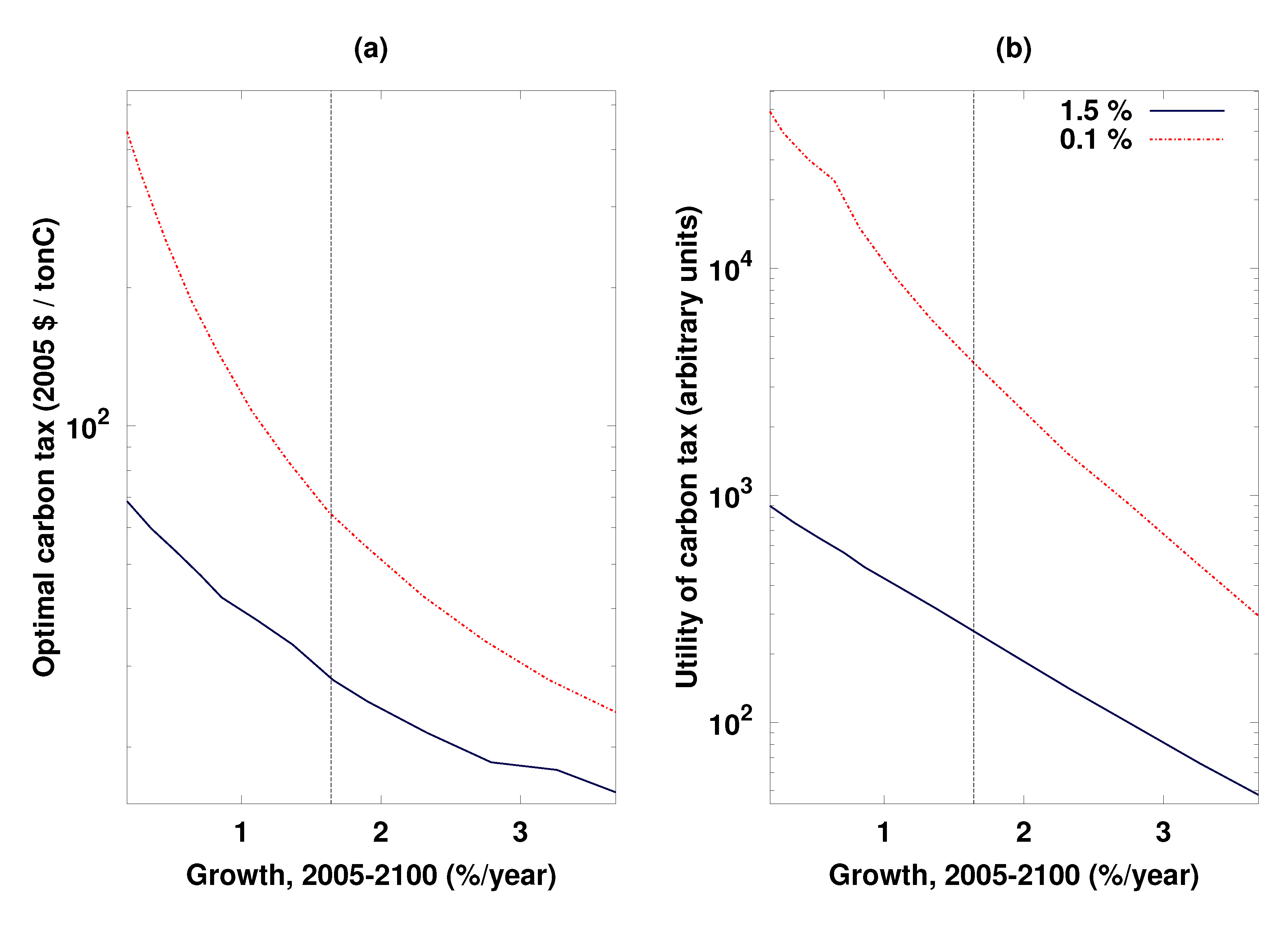The optimum carbon tax rate for the first time period, shown in Figure 2a, illustrates how assumptions about future economic growth affect the extent to which it is cost-effective to reduce greenhouse gas emissions now. The present optimum carbon tax rises as assumed future economic growth decreases, but this increase is rather slow for the range of economic growth values usually used in climate change studies: a decrease in assumed 21st century economic growth to 0.4%/year (from the default 1.6%/year) is needed to double the optimum tax from its default $28 per ton of carbon, while the higher economic growth rates featured in the SRES scenarios (1.9%–3.1%/year for 2005–2100) reduce the optimum tax level slightly to $18–25/tonC. The future utility loss from warming and, hence, the utility gain from emissions control now (Figure 2b), increases under slower economic growth, because a given fractional reduction in production due to warming is more burdensome in a relatively poor as compared to a wealthy society. In fact, the utility gain from emissions control is larger even though the assumed uncontrolled emission trajectory and, hence, the amount of greenhouse warming, is considerably lower under slow economic growth than under default economic growth. (Since the utility function in DICE is a transformation of global production trajectory intended to measure social welfare, for a given formulation of this function, we can think of the change in utility induced by climate policy as a qualitative indicator of the climate damage averted, although the absolute numerical utilities are arbitrary.)

Figure 2. Consequences of the assumed future economic growth rate for the optimal regulation of greenhouse gas emissions within the integrated assessment model DICE. In each panel, the solid (lower) line is for a discount rate (pure time preference) of 1.5%/year, and the dash-dot (upper) line is for a discount rate of 0.1%/year. The vertical dashed line indicates the growth rate under the default model assumptions (about 1.6%/year). The vertical axes are logarithmically scaled. (a) Optimal present-day (2000–2010) carbon tax (2005 $ per ton C) as a function of the assumed economic growth rate; (b) gain in utility (arbitrary units) under the optimal greenhouse gas control trajectory compared with no emission control, as a function of the assumed economic growth rate. With slower economic growth, climate change has a more marked effect on utility, and earlier and more stringent controls on greenhouse gas emission become cost-effective.

Figure 2. Consequences of the assumed future economic growth rate for the optimal regulation of greenhouse gas emissions within the integrated assessment model DICE. In each panel, the solid (lower) line is for a discount rate (pure time preference) of 1.5%/year, and the dash-dot (upper) line is for a discount rate of 0.1%/year. The vertical dashed line indicates the growth rate under the default model assumptions (about 1.6%/year). The vertical axes are logarithmically scaled. (a) Optimal present-day (2000–2010) carbon tax (2005 $ per ton C) as a function of the assumed economic growth rate; (b) gain in utility (arbitrary units) under the optimal greenhouse gas control trajectory compared with no emission control, as a function of the assumed economic growth rate. With slower economic growth, climate change has a more marked effect on utility, and earlier and more stringent controls on greenhouse gas emission become cost-effective.

The impact of economic growth assumptions on optimal emission trajectories in DICE is sensitive to several other parameters in the model, including the pure rate of time preference and the dependence of utility on income. The assumed 1.5%/year pure rate of time preference effectively attenuates the relevance of future generations’ suffering for present decisions [49]. If we now change the assumed pure rate of time preference to 0.1%/year, matching that used in Stern [7] and granting much more importance to the utility losses of future generations, the increase in the present optimum carbon tax rate with decreasing assumed future economic growth is sharper. The tax rate approximately doubles from its default (which at $65/tonC, is already more than double the $28/tonC optimum under a 1.5%/year rate of time preference) if assumed economic growth drops to 1.0%/year and quadruples for growth of 0.5%/year (Figure 2a).

The impact of the future economic growth rate on the optimal carbon tax is also importantly affected by the assumed dependence of utility on per-capita income. In DICE-2007, the marginal utility of an additional dollar of income is assumed to scale as the inverse square of current income, corresponding to an elasticity of two for the utility of consumption. (According to Nordhaus [50], the original DICE model from 1992 employed a value of one for numerical reasons, to improve the convergence of optimization runs.) This parameter is also known as the coefficient of relative risk aversion or of inequality aversion. 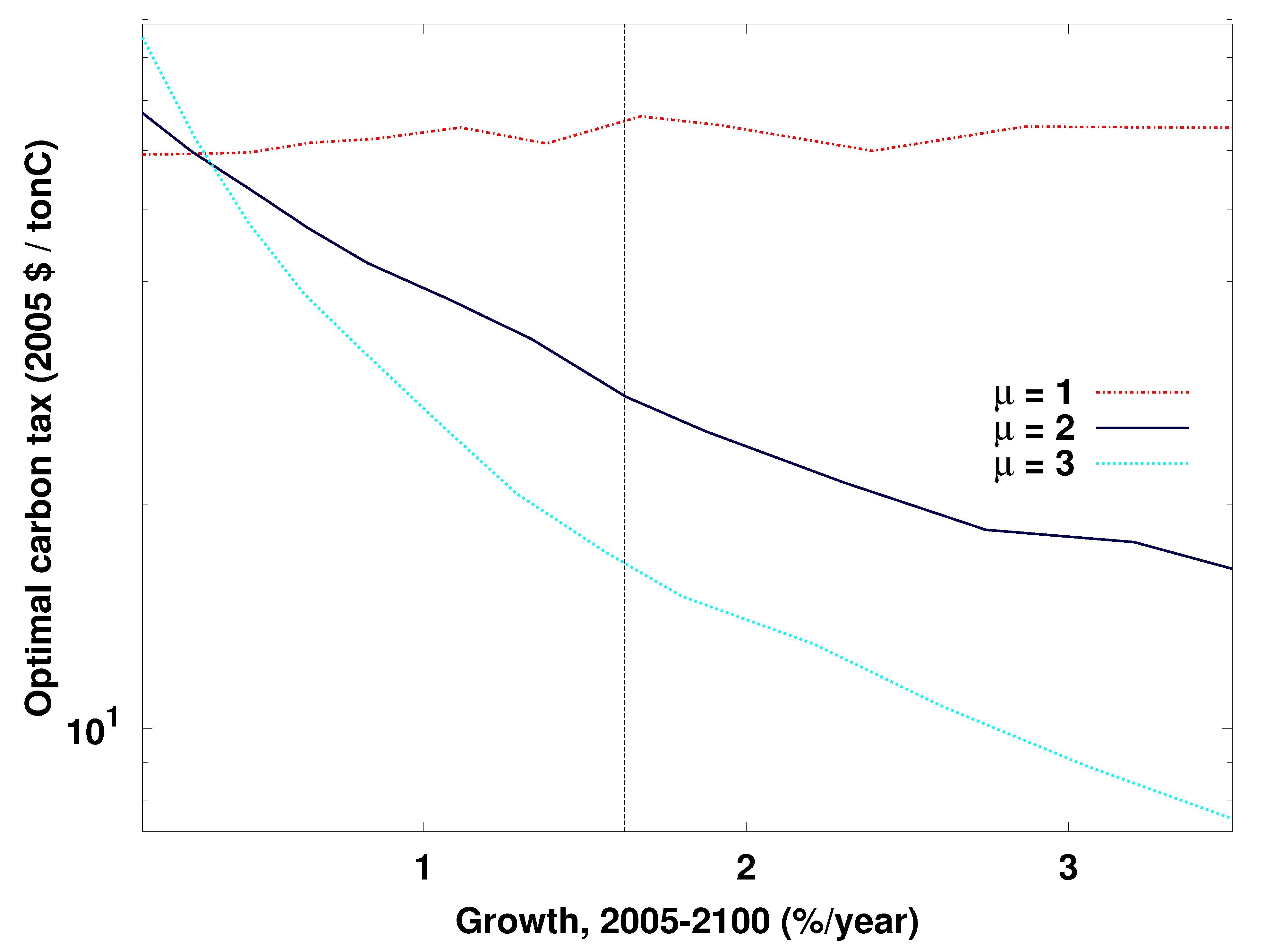A higher elasticity would increase the impact of economic growth on the utility loss induced by global warming and on the optimal carbon tax level (steepen the slopes of the curves in Figure 2), while a lower elasticity would decrease the impact. Thus, at an elasticity of three (and a discount rate of 1.5%), the optimal present-day carbon tax level triples from $17/tonC to $51/tonC as the assumed economic growth rate decreases from the default 1.6%/year to 0.4%/year, while at an elasticity of one, the optimal carbon tax level is about $60/tonC regardless of the assumed economic growth rate (Figure 3). While the exact value of this elasticity is arbitrary and empirical evidence on people’s preferences shows substantial variation [51], an elasticity of about two is generally regarded as reasonable [52] and is used in economic studies of such things as investment behavior [53,54] and spending on medical care [55]. Further, consistency with observed savings behavior may require higher elasticity values to be coupled with low rates of time preference [6], which is a combination of parameters that would tend to make the optimal carbon tax particularly sensitive to the economic growth trajectory.

While I have used the DICE model here because of its simplicity and straightforward description, simplifications made in DICE may lead to understatements of the benefit of emissions control policies under given assumed economic growth. DICE assumes that, for a given carbon tax level, emissions scale linearly with economic production, and that decarbonization of the economy occurs at a prescribed rate. In fact, if investment in research, development and infrastructure replacement is required to increase energy efficiency [10], energy efficiency may, as argued above, improve more slowly in slow-growth compared to high-growth scenarios, so that emissions per unit of production would be higher. As well, emissions reduction policies, such as a carbon tax, stimulate investment that decreases the unit cost of emission reductions over time, making a carbon tax more economically attractive than in a model like DICE, where no such “learning curve” exists [56,57,58]. Further work with DICE and with more complex models is therefore needed to understand the sensitivity of the numerical results reported here to parameter uncertainty and to model structural assumptions.

Figure 3. Optimal present-day (2000-2010) carbon tax (2005 $ per ton C) as a function of assumed economic growth rate under different assumed values of µ, the elasticity for the utility of consumption, and a discount rate (pure time preference) of 1.5%/year. The vertical dashed line indicates the growth rate under the default model assumptions (about 1.6%/year). The vertical axis is logarithmically scaled. The results shown in Figure 2 use µ = 2, the default value in the DICE model.

Figure 3. Optimal present-day (2000-2010) carbon tax (2005 $ per ton C) as a function of assumed economic growth rate under different assumed values of µ, the elasticity for the utility of consumption, and a discount rate (pure time preference) of 1.5%/year. The vertical dashed line indicates the growth rate under the default model assumptions (about 1.6%/year). The vertical axis is logarithmically scaled. The results shown in Figure 2 use µ = 2, the default value in the DICE model.

6. Conclusions

Long-term economic development is uncertain, and a variety of scenarios are plausible for changes in the size of various components of the world economy. Climate policy analyses must incorporate the full diversity of plausible future economic growth trajectories, including ones where economic growth slows or stops, as well as ones where economic growth continues in the context of technological and societal restructuring that allows massively increased production. Because the dependence of climate damages and the optimal carbon tax rates on future economic growth rate is close to, or more than, exponential (roughly straight, or concave up, lines in Figure 2a,b), even a moderate probability assigned to the lowest growth rates examined can substantially nudge the current climate policy seen as optimal toward immediate stringent controls on greenhouse gas emissions.

Under slow economic growth, growth in energy demand would be curtailed, which should slow climate change, but a shift to highly polluting fuels and a lack of capital to control emissions might offset some of the resultant reduction in emissions. Slow economic growth means that future generations will be less able to absorb the harms of climate change, which increases the urgency, and the likely payoff, of cutting emissions now through switching to renewable sources of energy and increasing the efficiency with which energy and materials are used to increase human welfare. Given that fossil fuel supplies are limited, investment in renewable energy has the double benefit of both reducing climate-change damage and putting the world economy on a more sustainable basis for continued growth in production.