1. Introduction
Energy is essential for socio-economic development and improvement of the quality of life. The use of fossil oil and other natural resources has resulted in detrimental impacts on the environment, especially through damage to the air, climate, water, land and wildlife [
1]. With increasing environmental consciousness and global demand for energy, the utilization of renewable and clean energy sources is necessary. Although the global economic recession has reduced the demand for energy currently, energy generation from renewable resources is still necessary for the environment and for the economy in the long term. Solar energy, one of the best renewable energy sources with the least negative impacts on the environment, is becoming a promising renewable energy source [
2].
The setup of a renewable energy power plant is a long process, from the very beginning stage of land survey and plant site selection, to the final stage of implementing and starting-up of the plant [
3]. Selecting a site for a renewable energy power plant is the very first and an important task. Some relevant studies are reviewed here. Azoumah
et al. [
4] listed six parameters for selecting a site for a concentrating solar power (CSP) plant: solar resource assessment, availability of water and cooling mode, soil structure and geology, land issues, geography and topography of the site, the energy demand profile and a grid-connected system. Aragonés-Beltrán
et al. [
3] used an analytic network process (ANP) to select the best photovoltaic (PV) solar power project based on risk minimization. Noone
et al. [
5] presented a tool for locating sites in hillside terrain for central receiver solar thermal plants based on field efficiency and average annual normal insolation. The calculation of field efficiency includes three factors: cosine efficiency, which is the ratio of the projected heliostat area in the direction of beam insolation to the surface area, shading and blocking losses. Halasah
et al. [
6] employed life-cycle assessment to evaluate the energy-related impacts of PV systems at different scales of integration. The input parameters included panel efficiency, temperature coefficient, shading losses, ground cover ratio and latitude, and the input data included hourly solar radiation, wind speed and temperature. Pavlovic
et al. [
2] studied the possibilities of generating electrical energy from on-grid PV solar systems of 1 kW in the Republic of Srpska, and the factors considered included yearly average values of the optimal panel inclination, solar irradiation on the horizontal, vertical and optimally-inclined plane, the ratio of diffuse to global solar irradiation, Linke turbidity, average daytime temperature and 24-h average temperature. Besarati
et al. [
7] assessed the potential of harnessing solar radiation in different regions of Iran by generating solar radiation maps for different surface tracking modes, and the result can be used for designing PV and CSP power plants. Phillips [
8] evaluated the sustainability for PV solar power plants by applying a mathematical model to the results of a qualitative-based environmental impact evaluation of the installation and operation of solar power plants. The impact categories include human health and well-being, wildlife and habitat, land use and geohydrological resources and climate change. Xiao
et al. [
9] constructed a site selection model for desert PV power plants using an analytic hierarchy process (AHP) and a geographic information system (GIS) in China. The major indices include climate, terrain, land cover and location, and each index contains several factors.
The evaluation and selection of an appropriate renewable energy plant site is a very complicated task, which involves the consideration of various qualitative and quantitative factors. In addition, if there are many plant sites available, the collection of relevant data from each site can be tedious or even impossible. Thus, this research proposes a two-stage evaluation model to evaluate the expected performance of renewable energy plant sites. In the first stage, a method that considers quantitative factors that are usually collectible is used to extract a number of candidate plant sites from many available plant sites. In the second stage, these candidate plant sites are further evaluated to consider qualitative factors and/or quantitative factors that are difficult to collect. The most suitable plant site can be selected as a result. To accomplish this goal, the comprehensive evaluation model is developed by integrating the AHP, data envelopment analysis (DEA), assurance region (AR) and fuzzy set theory. In the first stage, the ARs of the inputs and outputs are determined using fuzzy analytic hierarchy process (FAHP), and the DEA incorporated with AR is applied to evaluate the quantitative data of different sites. Based on the evaluation, the candidate plant sites are extracted. In the second stage, the FAHP is used to consider other qualitative data (or quantitative data that are difficult to collect), and the site with the highest priority is recommended for constructing the renewable energy plant. The flowchart of the proposed model is depicted in
Figure 1.
Figure 1.
Flowchart of the proposed model. AR, assurance region; FAHP, fuzzy analytic hierarchy process.
Figure 1.
Flowchart of the proposed model. AR, assurance region; FAHP, fuzzy analytic hierarchy process.
The rest of this paper is organized as follows.
Section 2 introduces the methodologies that are used for the model for renewable energy plant site selection.
Section 3 presents a case study in Taiwan to examine the practicality of the proposed model. Some concluding remarks are made in the last section.
3. Case Study
A two-stage evaluation model by integrating DEA and FAHP is constructed to assess various feasible sites for a renewable energy plant. In the model, the renewable energy plant site selection problem is defined first, and the factors for evaluating the suitability of various sites are selected next. Stage I is a plant site screening stage. Among many available plants sites, several candidate plant sites are selected by considering quantitative factors. This is done by applying the DEA-fuzzy AR method. In Stage II, the candidate plant sites are further evaluated to consider qualitative factors. By applying the FAHP, the most suitable plant site can be selected. A case study of the solar plant site selection in Taiwan is carried out using the proposed model.
Step 1: Define the renewable energy plant site evaluation problem: Experts in the renewable energy industry are invited to define the problem.
Step 2: Select the factors for evaluating renewable energy plant sites: A literature review, including solar energy conversion and renewable energy site selection, is carried out first [
33,
34,
35,
36,
37,
38,
39,
40], and experts in the solar energy industry in Taiwan are then interviewed to identify critical factors. The critical factors are considered and categorized into quantitative and qualitative factors. In Stage I, only quantitative factors are considered. As stated before, when applying DEA, inputs are critical factors that are smaller the better, and outputs are critical factors that are larger the better. Due to the information accessibility of various sites and the importance of various factors, we select two inputs and two outputs for the quantitative factors. The two inputs are temperature (I
1) and wind speed (I
2). The two outputs are sunshine hours (O
1) and elevation (O
2). The definitions of the inputs and outputs are listed in
Table 3. Because land is abundant and less expensive in southern Taiwan and sunshine is plentiful there, five counties (cities) with 15 towns/districts that are most suitable for setting PV solar plant sites are selected, namely A
1 to A
15, respectively. The data for these sites are listed in
Table 4. The potential locations are shown in
Figure 3.
Stage I: Selection of candidate solar plant sites using DEA-fuzzy AR: The CCR model is first applied on the case study. The results are shown in
Table 5.
Table 5 shows the efficiency and the rank of each DMU. The “Peers” column indicates the number of reference points that the DMU used to calculate its efficiency, and the “Reference set” lists the reference points to which the DMU is compared. Among the 15 DMUs, six of them are efficient with a value of one. For example, A
4 is efficient. Thus, it ranks the first among all DMUs. Since A
4 is located on the efficient frontier, its reference point is itself, and it does not have a peer to which to compare. A
1 has an efficiency value of 87.13, and it is not efficient. Its rank is 10. Its reference set includes two peers, A
9 and A
11. This means that A
1 is found inefficient when compared to A
9 and A
11.
Table 3.
Definitions of inputs and outputs.
Table 3.
Definitions of inputs and outputs.
| Factors | Definition |
|---|
| Inputs |
| Temperature (I1) | A numerical measure of hot or cold by detection of heat radiation. According to Radziemska [34], temperature increases lead to a decrease of the output power and of the conversion efficiency of the PV module. That is, the more sunshine a panel receives, the hotter the panel gets, and in turn, the conversion efficiency decreases. The heat factor can reduce output power by 10% to 25%, depending on the location and the equipment [39]. |
| Wind speed (I2) | Wind is the flow of gases on a large scale. Wind causes small particles to be lifted, and the suspended particles may impact the solar panels and equipment, which need to resist wind loads and uplift. Wind may cause erosion and operation failures of solar plants. |
| Outputs |
| Sunshine hours (O1) | A climatological indicator to measure the duration of sunshine in a period (here, a year) for a given location, typically expressed as an average of several years. The sunshine duration is the period during which direct solar irradiance exceeds a threshold value of 120 W/m² [35]. A longer sunshine duration can convert to a larger amount of output power. |
| Elevation(O2) | The height of a geographic location above sea level. A higher elevation means a shorter distance for solar radiation to reach the ground and a higher intensity of solar irradiance. A higher intensity of solar irradiance converts to a larger amount of output power. |
Table 4.
Quantitative data of the solar plant sites.
Table 4.
Quantitative data of the solar plant sites.
| County/City | Town/District | Temperature (°C) | Wind Speed (m/sec) | Sunshine Hours (h/year) | Elevation (m) |
|---|
| Yunlin County | A1 | 23.80 | 1.50 | 1779.47 | 31 |
| A2 | 23.43 | 1.73 | 1915.53 | 4 |
| A3 | 19.90 | 4.13 | 1452.00 | 8 |
| Chiayi County | A4 | 22.67 | 0.63 | 1588.63 | 265 |
| A5 | 16.87 | 0.40 | 976.43 | 130 |
| A6 | 23.47 | 3.27 | 2378.67 | 12 |
| Tainan City | A7 | 23.43 | 0.87 | 1718.00 | 21 |
| A8 | 23.70 | 4.53 | 2332.63 | 7 |
| A9 | 23.93 | 2.60 | 2320.03 | 12 |
| Kaohsiung City | A10 | 24.13 | 0.73 | 1605.17 | 51 |
| A11 | 23.60 | 0.23 | 1719.27 | 75 |
| A12 | 22.80 | 0.43 | 1605.20 | 253 |
| Pingtung County | A13 | 25.17 | 3.47 | 2029.70 | 27 |
| A14 | 24.57 | 0.60 | 1255.60 | 28 |
| A15 | 24.57 | 0.10 | 1560.80 | 16 |
Figure 3.
The potential locations in Taiwan.
Figure 3.
The potential locations in Taiwan.
Table 5.
DEA performance results. DMU, decision-making unit.
Table 5.
DEA performance results. DMU, decision-making unit.
| DMU | Efficiency | Rank | Peers | Reference Set |
|---|
| A4 | 100 | 1 | 0 | A4 |
| A6 | 100 | 1 | 0 | A6 |
| A9 | 100 | 1 | 0 | A9 |
| A11 | 100 | 1 | 0 | A11 |
| A12 | 100 | 1 | 0 | A12 |
| A15 | 100 | 1 | 0 | A15 |
| A8 | 97.1 | 7 | 1 | A6 |
| A2 | 92.4 | 8 | 2 | A9, A11 |
| A7 | 92.27 | 9 | 2 | A9, A11 |
| A1 | 87.13 | 10 | 2 | A9, A11 |
| A10 | 85.44 | 11 | 2 | A9, A11 |
| A13 | 81.38 | 12 | 2 | A4, A6 |
| A5 | 80.05 | 13 | 3 | A9, A11, A12 |
| A3 | 72.08 | 14 | 2 | A4, A6 |
| A14 | 66.9 | 15 | 2 | A9, A11 |
As mentioned before, the conventional DEA cannot incorporate experts’ opinions on the importance of the inputs/outputs; thus, DEA-fuzzy AR is applied next to the case study. The FAHP is used to set the ARs for the inputs and outputs first, and then, the DEA/AR is applied to calculate the efficiencies of the solar plant sites. Eight experts in the solar industry were asked to pairwise compare the importance of the inputs/outputs. A question, such as “which input is more important in selecting the location of the solar plant site and how much more?” was asked, and a pairwise comparison with five linguistic terms was used. The comparison matrix for the inputs by the first expert by applying Equation (18) is shown as follows:
All experts’ opinions are synthesized using the geometric average method, and the fuzzy aggregated pairwise comparison matrix of the inputs by applying Equation (19) is:
The fuzzy aggregated pairwise comparison matrix of the inputs is transformed into a defuzzified aggregated pairwise comparison matrix using the center of gravity (COG) method (Equation (20)). By applying Equation (21), the aggregated pairwise comparison matrix is:
By applying Equation (22), the maximum eigenvalue and the eigenvector for the defuzzified aggregated pairwise comparison matrix of the inputs are:
Because there are only two inputs, the pairwise comparison is always consistent, and the CI and CR calculations are not necessary. If the number of inputs is equal to or more than three, the consistency test must be performed.
Two matrices are formed based on the fuzzy aggregated pairwise comparison matrix in Equation (27): one contains all low values in the fuzzy matrix, and the other contains all high values in the fuzzy matrix.
The priorities of the inputs under the two matrices are calculated using Equation (31), and they are:
The same procedure is carried out to calculate the priorities of the outputs, and they are:
For temperature (I
1), the priority ranges from 0.715 to 0.863,
i.e., I
1 = [0.715, 0.863]. For wind speed (I
2), the priority ranges from 0.138 to 0.285,
i.e., I
2 = [0.138, 0285]. For sunshine hours (O
1), the priority ranges from 0.762 to 0.871,
i.e., O
1 = [0.762, 0.871]. For elevation (O
2), the priority ranges from 0.129 to 0.238,
i.e., O
2 = [0.129, 0.238]. Based on the AR concept discussed before [
21,
22,
25], the AR for each pair of inputs and each pair of outputs can be calculated as shown in
Table 6 and
Table 7.
Table 6.
Assurance range (AR) for inputs.
Table 6.
Assurance range (AR) for inputs.
| Input Ratio | Lower Bound | Upper Bound |
|---|
| wI1/wI2 | 0.715/0.285 = 2.509 | 0.863/0.138 = 6.254 |
Table 7.
Assurance range (AR) for outputs.
Table 7.
Assurance range (AR) for outputs.
| Output Ratio | Lower Bound | Upper Bound |
|---|
| wO1/wO2 | 0.762/0.238 = 3.202 | 0.871/0.129 = 6.752 |
Table 8.
DEA-fuzzy AR performance results.
Table 8.
DEA-fuzzy AR performance results.
| DMU | Efficiency | Rank | Peers | Reference Set |
|---|
| A12 | 100 | 1 | 0 | A12 |
| A4 | 94.11 | 2 | 1 | A12 |
| A11 | 91.14 | 3 | 1 | A12 |
| A5 | 76.55 | 4 | 1 | A12 |
| A15 | 54.43 | 5 | 1 | A12 |
| A10 | 53.28 | 6 | 1 | A12 |
| A1 | 39.61 | 7 | 1 | A12 |
| A14 | 35.12 | 8 | 1 | A12 |
| A13 | 34.29 | 9 | 1 | A12 |
| A7 | 32.21 | 10 | 1 | A12 |
| A6 | 20.19 | 11 | 1 | A12 |
| A9 | 19.92 | 12 | 1 | A12 |
| A3 | 14.99 | 13 | 1 | A12 |
| A8 | 12.26 | 14 | 1 | A12 |
| A2 | 7.44 | 15 | 1 | A12 |
Using the ARs in
Table 6 and
Table 7, DEA is run to evaluate the efficiencies of the solar plant sites. As seen in
Table 8, the result shows that, considering experts’ opinions on the importance of the inputs and outputs, only one plant site, A
12, is efficient, instead of six under the conventional DEA. Under the DEA concept, only the DMU with an efficiency of 100% is treated as efficient. Therefore, all DMUs except A
12 are inefficient. The results are generated from the DEA-fuzzy AR model, and only A
12 is located on the efficient frontier. The other DMUs, when compared to A
12 as a reference point, are found inefficient. Two other DMUs that have higher efficiency scores are A
4 and A
11, with efficiencies of 94.11 and 91.14, respectively. The efficiencies of all other solar plant sites are less than 77. Because the selection of solar plant site cannot only consider quantitative factors, many other qualitative factors need to be considered, too. Therefore, in this stage, three plant sites that have higher efficiency scores and that outperform others are selected for further analysis.
The selection of these three plant sites is done arbitrarily by the authors. If there are several DMUs that are 100% efficient, they will be automatically selected for the evaluation in the next stage. In this case, however, only one plant site is efficient under the first-stage analysis. Since both quantitative and qualitative factors should be considered in the problem, the selection of plant A12 is based on only quantitative factors, and completing the evaluation process without going through Stage II analysis is not recommended. Therefore, more efficient DMUs are selected in this stage. Since the efficiency difference between A11 (ranked third) and A5 (ranked fourth) is 14.59%, a rather large number, A5 is not selected for the next-stage evaluation.
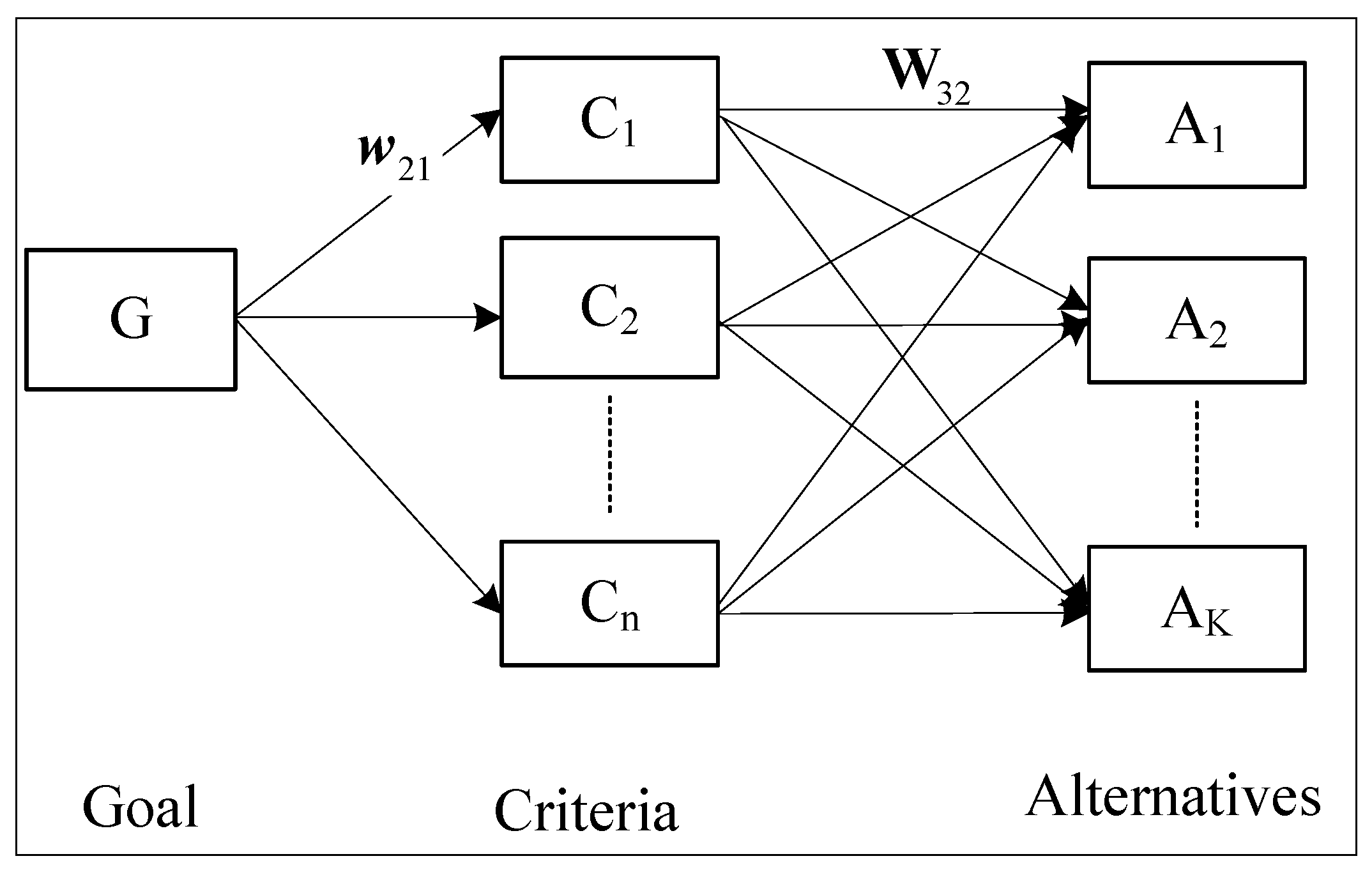
Stage II: Selection of the most suitable solar plant site using FAHP: In Stage I, inputs and outputs are all quantitative factors. In Stage II, factors that are qualitative in nature or quantitative but difficult to measure or collect are considered here. With a comprehensive literature review and consultation with experts in the industry, the factors for determining the suitability of solar plant sites are collected, and a hierarchy is constructed, as shown in
Figure 4. Under the goal, there are three criteria, each of which has several detailed criteria. For example, under criterion costs (C
2), the detailed criteria are land cost (D
21), construction cost (D
22), equipment cost (D
23), operation and maintenance cost (D
24) and electric power transmission cost (D
25). The definitions of the detailed criteria are listed in
Table 9. The three solar plant sites generated in Stage I are the alternatives.
Table 9.
Definitions of detailed criteria.
Table 9.
Definitions of detailed criteria.
| Detailed Criteria | Definition |
|---|
| Support mechanisms (D11) | Different government policy instruments have been implemented to support solar PV power plants. Some incentives include feed-in-tariffs, investment tax credits, subsidies and favorable financing. The incentives may be different at different locations. |
| Protection laws (D12) | The existing laws and regulations might constrain the development of solar plants in different areas, such as farm land and inhabited areas. |
| Service life (D13) | Expected useful life of PV solar plant. The electricity buy-back period may be different, and the weather and geological conditions, such as temperature, humidity, salt-laden air, may affect the service life of the solar plant. |
| Land cost (D21) | The cost of obtaining the land required for setting up the solar plant. |
| Construction cost (D22) | The total cost for constructing the solar plant, including all of the capital expenses related to the initial establishment of the plant, such as buildings, roads, etc. |
| Equipment cost (D23) | Costs for the initial purchase and installation of the equipment and facilities. |
| Operation and maintenance cost (D24) | Costs for everyday operation of the solar plant and repair and maintenance, including labor, material, etc. |
| Electric power transmission cost (D25) | The transfer cost of electrical energy from the solar power plant to electrical substations located near demand centers. |
| Human well-being (D31) | The negative impacts of the solar plant on the health of the residents and aesthetics in the area. |
| Wild life and habitat (D32) | The negative impacts of the solar plant on the animal inhabitants and plants in the area. |
| Topography (D33) | A description of relief or terrain, the three-dimensional quality of the surface, and the identification of specific landforms of a place. A solar plant needs to be built in a flat place where solar radiation can be reached easily. |
| Land availability (D34) | The availability of land for setting up a solar plant with economies of scale and for future expansion. |
A questionnaire is prepared, and the eight experts are invited to fill out the questionnaire; the results from each expert can then form pairwise comparison matrices. After the calculation, we can obtain the priorities of the eigenvectors for defuzzified aggregated pairwise comparison matrices, as shown in
Table 10. Among the three criteria, costs (C
2) have the highest priority with 0.493, followed by policies (C
1) with 0.269 and environment conditions (C
3) with 0.238. This implies that when selecting the most appropriate solar plant site, the overall costs for constructing and running the solar plant in a certain site are considered the most important criterion by the experts. Under the policies (C
1) criterion, service life (D
13), with a priority of 0.466, is the most important detailed criterion, followed by support mechanisms (D
11) with a priority of 0.319 and protection laws (D
12) with 0.215. Service life estimates the expected useful life of the PV solar plant and ultimately determines the duration and amount of power generation of the plant. Therefore, it is a rather important detailed criterion. Under the costs (C
2) criterion, operation and maintenance cost (D
24), with a priority of 0.382, is the most important detailed criterion. Land cost (D
21) ranks the second (0.190), followed by electric power transmission cost (D
25) with a priority of 0.177 and construction cost (D
22) with a priority of 0.171. Operation and maintenance cost (D
24) occurs continuously as long as the solar plant is under operation. The costs for everyday operation of the solar plant and repair and maintenance, including labor and material, depend on the transportation cost and the availability of human resources in that area. Therefore, a good plant site can reduce the expected long-term operation and maintenance cost. Under the environment conditions (C
3) criterion, wild life and habitat (D
32) has the highest priority with 0.432. Human well-being (D
31) with a priority of 0.362 ranked the second. Due to the rise of environmental awareness, environment impact assessment is necessary before a solar plant is allowed to be constructed. Thus, the negative impacts of the solar plant on the animal inhabitants and plants and on human well-being in the area need to be considered seriously.
The synthesized priority of a detailed criterion, which is calculated by multiplying the priority of the detailed criterion by the priority of its upper-level criterion, shows the overall importance of the detailed criterion. The most important detailed criterion is operation and maintenance cost (D24), with a priority of 0.188, followed by service life (D13) and wild life and habitat (D32), with priorities of 0.125 and 0.103, respectively. Some other important detailed criteria include land cost (D21) (0.094), electric power transmission cost (D25) (0.087), support mechanisms (D11) (0.086) and human well-being (D31) (0.086).
Table 10.
Priorities of factors.
Table 10.
Priorities of factors.
| Criteria | Detailed Criteria | Priorities | Rank | Synthesized Priorities | Synthesized Rank |
|---|
| Policies (C1) (0.269) | Support mechanisms (D11) | 0.319 | 2 | 0.086 | 6 |
| Protection laws (D12) | 0.215 | 3 | 0.058 | 9 |
| Service life (D13) | 0.466 | 1 | 0.125 | 2 |
| Costs (C2) (0.493) | Land cost (D21) | 0.190 | 2 | 0.094 | 4 |
| Construction cost (D22) | 0.171 | 4 | 0.084 | 8 |
| Equipment cost (D23) | 0.080 | 5 | 0.040 | 10 |
| Operation and maintenance cost (D24) | 0.382 | 1 | 0.188 | 1 |
| Electric power transmission cost (D25) | 0.177 | 3 | 0.087 | 5 |
| Environment conditions (C3) (0.238) | Human well-being (D31) | 0.362 | 2 | 0.086 | 6 |
| Wild life and habitat (D32) | 0.432 | 1 | 0.103 | 3 |
| Topography (D33) | 0.144 | 3 | 0.034 | 11 |
| Land availability (D34) | 0.062 | 4 | 0.015 | 12 |
Table 11 shows the expected performance of the solar plant sites under each criterion. For example, under support mechanisms (D
11), A
11 has the highest priority of 0.626, followed by A
12 and A
4, with priorities of 0.231 and 0.143, respectively. The solar plant site that performs the best under a sub-criterion is highlighted in gray in
Table 11. Solar plant site A
4 performs the best under five sub-criteria: service life (D
13), land cost (D
21), construction cost (D
22), human well-being (D
31) and wild life and habitat (D
32). Solar plant site A
11 performs the best under six sub-criteria: support mechanisms (D
11), equipment cost (D
23), operation and maintenance cost (D
24), electric power transmission cost (D
25), topography (D
33) and land availability (D
34). Solar plant site A
12 performs the best under one sub-criterion only,
i.e., protection laws (D
12).
Finally, the overall priorities of the solar plant sites are obtained by synthesizing the priorities. For example, the overall priority of A
4 is calculated as follows:
The priorities of A11 and A12 are 0.402 and 0.245, respectively. The result shows that A11 has the highest overall priority. Therefore, A11 should be selected for building the solar plant.
Table 11.
Priorities of solar plant sites.
Table 11.
Priorities of solar plant sites.
| Criteria | Detailed Criteria | Synthesized Priorities | A4 | A11 | A12 |
|---|
| Policies (C1) | Support mechanisms (D11) | 0.086 | 0.143 | 0.626 | 0.231 |
| Protection laws (D12) | 0.058 | 0.176 | 0.375 | 0.449 |
| Service life (D13) | 0.125 | 0.478 | 0.333 | 0.189 |
| Costs (C2) | Land cost (D21) | 0.094 | 0.557 | 0.188 | 0.255 |
| Construction cost (D22) | 0.084 | 0.392 | 0.374 | 0.233 |
| Equipment cost (D23) | 0.040 | 0.318 | 0.465 | 0.216 |
| Operation and maintenance cost (D24) | 0.188 | 0.267 | 0.539 | 0.195 |
| Electric power transmission cost (D25) | 0.087 | 0.300 | 0.425 | 0.275 |
| Environment conditions (C3) | Human well-being (D31) | 0.086 | 0.385 | 0.311 | 0.304 |
| Wild life and habitat (D32) | 0.103 | 0.447 | 0.304 | 0.250 |
| Topography (D33) | 0.034 | 0.381 | 0.394 | 0.225 |
| Land availability (D34) | 0.015 | 0.277 | 0.481 | 0.241 |
| Synthesized priorities | - | - | 0.353 | 0.402 | 0.245 |


