Optimal Control Approaches to the Aggregate Production Planning Problem

Abstract

In the area of production planning and control, the aggregate production planning (APP) problem represents a great challenge for decision makers in production-inventory systems. Tradeoff between inventory-capacity is known as the APP problem. To address it, static and dynamic models have been proposed, which in general have several shortcomings. It is the premise of this paper that the main drawback of these proposals is, that they do not take into account the dynamic nature of the APP. For this reason, we propose the use of an Optimal Control (OC) formulation via the approach of energy-based and Hamiltonian-present value. The main contribution of this paper is the mathematical model which integrates a second order dynamical system coupled with a first order system, incorporating production rate, inventory level, and capacity as well with the associated cost by work force in the same formulation. Also, a novel result in relation with the Hamiltonian-present value in the OC formulation is that it reduces the inventory level compared with the pure energy based approach for APP. A set of simulations are provided which verifies the theoretical contribution of this work.

1. Introduction

Nowadays one of the most important challenges faced by business is the adjustment of firm resources in order to satisfy market requirements subjected to fluctuations over time, namely costs, prices, existences, demands, etc. [1]. In the case of facing fluctuating, hard-to-predict demand, several companies around the world have the conflicting goals of (1) limiting the buildup in finished goods inventory; and (2) minimizing changes in the capacity level. Traditionally, the most economical solution to absorb fluctuations in demand is a mix of two alternatives [2,3]:

• Adjust the capacity level (hiring/firing labor force, working overtime/undertime, subcontracting, etc.); this is known as the chase alternative [4,5]: track the expected monthly sales and compute the corresponding capacity requirements.
• Use of inventories (excess of SKUs, backlog of orders, or lost sales); this is known as the level plan: maintain a steady production rate over the entire year, using finished goods (smoothing/anticipation) stocks to absorb ongoing differences between output and sales.

This problem—known as the aggregate planning problem—can be stated as follows [6,7,8,9]:

• determine simultaneously the production rate P, inventory level $\mathsf{\beta }$, and capacity levels C,
• for meeting a fluctuating demand (a set of forecasts),
• at each period of a finite planning time horizon in days (t = 1,2,..., N),
• for a given set of production resources,
• involving one product or a family of similar items (with small differences so that considering the problem from an aggregate viewpoint is justified),
• while minimizing total relevant costs (i.e., payroll, hiring/layoffs, overtime/undertime, inventory/shortage, etc.),
• and subject to non-constant, time varying constraints.

Aggregate production planning (APP, or workforce planning, production and employment smoothing, capacity and production planning), deals with matching capacity (via adjustment of production load, inventory, and employment levels) to changing demand, over a finite planning horizon, in order to achieve long-run profitability. By converting monthly sales forecasts, inventory levels, labor inputs, and production rates—of a single entity with characteristics representative of an entire product group—to a convenient aggregate load/capacity format (such as standard hours), a production plan is generated [10]: this involves a tradeoff between penalties for carrying inventory and varying the capacity level incurs the minimum total marginal cost over a calendar year. Because of this, the aggregate planning process has an economic importance due to the decisions involved (regarding the capacity and inventory levels necessary to meet anticipated demand over the planning period), as they impact the company’s performance, i.e., profit maximization. This in turn requires complete and accurate information about: machine capacity, labor utilization, levels (inventory, safety stock, manpower adjustment, subcontract, storage), time (regular/overtime), costs (production, inventory, overtime/idle time, subcontracts, shortage, lost sales, break down, backorder, hiring/firing/training). With this idea on mind, the next section presents a discussion of APP in production-inventory systems, while Section 3 introduces the research statement of APP as a control engineering problem in the context of optimal control theory. In Section 4, the stability analysis and mathematical modeling of APP is present. In order to show the validity and usefulness of the proposed formulation, results are presented in Section 5. Finally, Section 6 shows the conclusions derived from the case study plus future research venues.

2. APP in Production-Inventory Systems

2.1. Decision Science Approaches to the Aggregate Planning Problem

Models that have been used to solve the APP problem include: linear decision rule (for long-term strategic APP decisions), transportation model, dynamic programming, lot sizing model, linear programming (the most widely accepted method like in ([11]), , heuristics [12], simulation [13], goal programming [14], micro spreadsheet analysis [15], multi-objective optimization [16], fuzzy formulation models [17,18], genetic algorithms (GAs) [19], and multiple criteria mixed integer programming [20]. Based on Holt et al., in [2], in the area of models for planning/scheduling production-inventory systems, two types of models can be identified:

• Static models which are based on a finite planning horizon, considering deterministic demand. In this scenario, the receding planning horizon is bigger than the period by period plan.
• Dynamic models which consider a indefinite planning horizon, with a proper forecasting in demand; this based on the context that period by period decisions are based on a receding forecast over a planned time horizon.

where most of the existing aggregate planning models found in the literature [21]:

• Try to minimize an objective function representing “total relevant costs” (like production, inventory, shortage costs) over the fixed planning horizon.
• The usual constraints employed are inventory and capacity constraints, and are formulated to a single-objective function in linear programming [22].

A review of the literature over the past 20 years, in the area production planning modeling, shows the following: a taxonomy of the mathematical models used in aggregate planning; a literature review in aggregate, disaggregate, scheduling, and sequencing methods by feature, model, objectives, decision variables, and solution method; the achievements in optimal control methods—based on the maximum Pontryagin´s principle theory—that allowed analytical investigation of aggregate production planning systems to be carried out in order to gain an insight into their optimal behavior; and the literature in aggregate production planning models that have been introduced in the last four decades; the different planning models used in the production arena—from the supply chain level down to the manufacturing resource and capacity—as well the different approaches followed (namely conceptual, analytical, etc.) are summarized in [23]. In recent years, it has become evident that many researchers and practitioners are increasingly aware of addressing:

• Real-life situations of management and decisions with the presence of multiple objectives; by developing goal programming optimization models.
• Variations over time; by developing multi-period optimization models.
• Novel optimization methods as convex optimization in [24].

Even though all of the APP models cited in the literature have shown good performance in the academic field that have not in practical life, according to [25] the following reasons that apply are:

• Current models do not capture the real world approaches in APP scenarios.
• The hypothesis in which items are homogeneous and are aggregated.
• The hypothesis that workforce has the same competence.
• In the mathematical modeling, the following areas are not considered, such as: human resources, marketing, and finance.
• The information provided by industry is not proper in the context of sales forecasting and cost information.
• Complex mathematical modeling and analysis of the APP process.

Furthermore, in [26] the following reasons apply:

• The hypothesis that uniform rates are assumed for different items, which do not capture the scenario for producing various items.
• There is an absence of interest from managers to adapt mathematical methods and proper techniques.
• The cost related to the collection and quantification of data in order to apply the above techniques.
• The real cost functions in organizations are not well established by actual techniques.

Each of the last mentioned issued can be grouped as follows:

• Regarding the modeling approach; based on [27], decision makers such as operations researchers and other mathematical decision builders and its application in real scenarios are far from business practice.
• Regarding the aggregation approach; even though it intends to (1) simplify/facilitate the myriad of calculations, and (2) to reduce the solving time of a large problem, it presents some issues [28]: aggregation does not result in a better optimal solution; it probably compromises optimality and may even result in an infeasible solution; it usually results in a better attained solution within a fixed solution time.
• Regarding the use of mathematical models; comments in journals indicate that because a worrying gap exists between theory and practice, as mathematical (optimizing) models have not had a significant impact on industry operations management practices managers find mathematical methods too daunting; the cost assumptions used in models are over-simplified and unrealistic; simplified/inflexible assumptions which limit their industrial applicability; cannot cope with calendar variations (i.e., holidays), and the revision of distant, and therefore, speculative forecasts cause instability in the schedules; broader concepts in the area of employment policy and inventory practices need to be introduced.

Summarizing: due to the highly complex constraints of the APP problem, exact optimal solutions provided by traditional optimization methods may very possibly be meaningless. It is true that a number of artificial intelligence approaches—combined with mathematical programming models—have been used to solve the APP problem, but little attention has been given to the consideration that marks the difference between a pure academic treatment of the APP problem and a result with real-life, practical implications: the simultaneous combination of many constraints affecting the quality of the APP. Based on this, in its simplest form the production planning paradigm describes firm operating in a market facing external demand which it tries to meet by utilizing a limited set of production resources that has limited ability to generate output in a given time period [29]. In this context, the application of optimal control approaches presents a suitable mathematical tool with the intention to model and analyze the APP problem in a short time horizon, which is our case of analysis. Also, it is important to establish that optimal control is a dynamic optimization problem which can handle several decision variables and a control law in order to set up the conditions for a decision maker in the production planning context.

2.2. The Dynamic Nature of APP

The previous sections can be summarized as follows: an economical solution (for companies) to deal with a fluctuating demand is a mix between the chase alternative (hire/fire capacity) and level plan (inventory excess/shortages) strategies. This involves an inventory-capacity tradeoff, and is known as the aggregate planning problem: determine what must be the production rate, inventory and capacity levels necessary to minimize inventory holding, shortages, and production switching costs subject to time varying constraints. To address this problem, static and dynamic models—which try to minimize a linear programming objective function subject to inventory and capacity constraints—have been proposed. More recently, and in order to reflect more realistic situations, models with multiple objectives and variations over time, have been developed. As mentioned before, the proposed approaches have several shortcomings: they are over-simplified and unrealistic, attained solutions may be even impractical and infeasible, the use of speculative forecasts causes instability in the obtained schedules, etc. However, it is the premise of this paper that the main drawback of these proposals is, that they do not take into account the dynamic nature of the aggregate planning problem: the excessive inventory and production costs due to the use of speculative forecasts, is worsened by a poor understanding of the time lags between the ordering of goods and receipt into stock [30,31]. In fact, a production system designed to deal with the APP problem should have as objectives:

• to buffer the production system from the customer; with a minimum reasonable inventory that absorbs the high frequency content in demand and allows having a level schedule. In this way, the variability of customer demand is reduced/avoided as switching production levels up and down frequently may be very expensive in practice [32].
• to buffer the customer from supply time lags; by selling goods straight off the shelf. In this way high customer service levels can be achieved, which can only be accomplished when the dynamic behavior of its constituent parts (i.e., materials/information flow, operations performed, resources/decision, rules/performance measures used) has been taken into account [33].
• Demand patterns; after a ramp increase there is a continuing freefall in inventory levels, after a step increase there is a permanent inventory deficit. So demand—without some form of averaging—results in excessive fluctuations in production rates (which are supposed to be absorbed by the inventory buffers).
• Lead times; the amount of inventory holding that is needed to satisfy a customer service level is dependent on the uncertainties in both demand and lead times.
• Inventory levels; trying to correct all the inventory discrepancy in a single time period, when in fact it may take many more time periods, provokes excessive (overshoots and undershoots around the target level).

3. Research Statement

3.1. Control Engineering & Production/Inventory Control

In [34] the author presents a series of reasons for using control engineering techniques in production/inventory control, i.e., the use of standard forms, the block diagram format, standard techniques that enable important performance metrics to be calculated without recourse to simulation, there are a number of techniques for transferring problems from one domain into another, etc. Authors like [35,36,37,38,39] present in-detail reviews of control engineering applications to production/inventory control. One of these applications that deserves to be mentioned apart—due to the number of research studies based on it—is the APIOBPCS concept. APIOBPCS stands for Automatic Pipeline, Inventory and Order Based Production Control System, and it is a well-established (both industrially and theoretically) production scheduling/control system model which operates on a knowledge of customer demand, inventory level, and unfilled orders, and that it provides an acceptable trade-off between production smoothing and a high level of stock turnover. The ordering policy/production algorithm of APIOBPCS is representative of work in [40]. Most of the APIOBPCS research has been undertaken using both control theory mathematics and system dynamics (SD), the most representative works in SD are present in [41] where it is applied to APP via transfer function approach; in [42] applying SD for production-inventory systems; in [43] a production-inventory system for APP described by differential equations via control oriented approaches; and in [44] where the SD approach is extended in production-inventory in remanufacturing. Based on this, APIOBPCS models are usually expressed in a continuous control form, but there is a discrete version available as well. In any case, the APIOBPCS simulation models may be used confidently as a benchmark to demonstrate performance enhancement for a wide range of practical scenarios [45].

3.2. Order-Up-To (OUT) and Smoothing Policies

As inventories should have a stabilizing effect on material flow patterns, a minimum reasonable inventory is necessary to absorb the variations in demand and allow a level schedule. The level scheduling problem (LSP), or production smoothing problem (PSP), refers to the problem of finding level schedules where:

• production of a given product is constant over time or,
• the cumulative production amount of a product is proportional to time or,
• the items should be dispersed over the schedule as uniformly as possible, with a minimal total deviation from the final level of operations.

Setting a takt-paced production results in a leveled production/production smoothing (key to establish the strategic/market pull), which is a simple matter of buffering—with either a time backlog or inventory—the production line from demand variability. The tradeoff between stocks and schedule stability is reflected in the master production schedule. On the other hand, a replenishment strategy that strives to bring the inventory position up to a predetermined target level is called an OUT policy. These kind of policies are very popular both in research as in practice since they are known to minimize inventory holding and shortage costs. Dejonckheere, et al. [39] presents two shortcomings of OUT policies are:

• Generation of a bullwhip effect.
• If production is not flexible and costs are excessive, a not optimal option is present.

Regarding point 1; the bullwhip effect has largely been analyzed by the OR, system dynamics, and control theory communities, where two popular approaches are: the statistical inventory control approach and the control engineering approach. Most of the research developed analyzing bullwhip effect considered supply chain systems. However, from the point of view of production-inventory systems the bullwhip effect has been studied in [46] where it applies autoregressive models to achieve multiple steps demand; in [47] an adaptive base-stock policy to determine order quantities; and in [48] explores the inventory stability in the context of a seasonal supply chain. In the case of the first approach: steady-state models based on steady-state conditions—like deterministic, stochastic, economic game-theoretic, and simulation models—are insufficient and therefore, unable to describe, analyze, and find remedies for problems like the bullwhip effect. In the case of the second approach: the bullwhip effect can be avoided by smoothing the ordering pattern—a problem known in the literature as the “production smoothing problem”—which means that it is possible to dampen order fluctuations even in environments where decision makers have to rely on forecasts.

Regarding point 2; the total costs of a perfectly controlled system—defined as a system that faithfully tracks some reference or target signal [49], is composed by costs associated with perfectly tracking the target (i.e., traditional fixed and variable costs), and costs associated with not being in perfect control of a system (i.e., under produce/over produce costs, and excessive/insufficient inventory costs). As there is trade-off to be made between OUT policies’ minimum inventory holding plus shortage costs, and smoothing policies’ minimum production switching costs, when the cost structure is altered, there is a need to identify a set of values (related to the production rate, and inventory/capacity levels) that reduce the sum of total costs [50].

3.3. The Aggregate Planning Problem as an Optimal Control Problem

Fact #1: the aggregated planning problem has to do with finding an optimal set of parameters’ values that minimizes a set of costs, facing a varying demand and within a finite planning time horizon; fact #2: the control engineering approach allows to analyze, design and simulate dynamic models; fact #3: in order to dampen order fluctuations and avoid the bullwhip effect (generated by OUT policies), a smoothing policy is required. When viewed together, these facts suggest (1) the understanding of the aggregated planning problem as an optimization problem; and (2) the use of control engineering-based tool capable of dealing with dynamic systems that allows the characterization of damping strategies. With this idea on mind, we state the research proposal of this paper as the formulation of APP as an optimization problem, applying OC techniques via an energy-based formulation for the dynamical system which describes the behavior and nature of the problem.

4. Stability and Mathematical Modeling for APP

4.1. Mathematical Modeling of APP

Based on a previous work [51], and [52] which applies second-order differential equation analogizing production system with mechanical vibration systems, here the approach is to propose an energy based analogy to obtain the dynamic equation for APP in production-inventory systems. In order to develop a consistent energy based analogy for APP, the following energy based function for APP, where $E_{APP}$ is the total energy of the APP system which is proposed: $E_{APP}=\frac{1}{2}C{\stackrel{•}{P}}^2+{\displaystyle \underset{Po}{\overset{P}{\int }}W\left(P\right)dP}$. Considering the Kinetic and Potential energy, where the Kinetic energy is such as: $T=\frac{1}{2}C{\stackrel{•}{P}}^2$, and the potential energy is calculated as: $V=\frac{1}{2}W{P}^2$, where in our analysis $W\left(P\right)=WP$. The Lagrangian is:

$$L\left(P,\stackrel{•}{P}\right)=T-V=\frac{1}{2}C{\stackrel{•}{P}}^2-\frac{1}{2}W{P}^2$$

(1)

Calculating the Lagrangian equation is:

$$\frac{d}{dt}\left(\frac{\partial L}{\partial \stackrel{•}{P}}\right)-\left(\frac{dL}{dP}\right)=\mathsf{\varphi }$$

(2)

From where, for stability purposes, the damping is of the form: $\mathsf{\varphi }=-\left(\mathsf{\beta }\left(t\right)-\mathsf{\alpha }\right)\stackrel{•}{P}$. Finally, for purposes of APP, the equation of the system is the following model:

$$C\frac{d^{2}P}{d{t}^2}+\left(\mathsf{\beta }(t)-\mathsf{\alpha }\right)\frac{dP}{dt}+WP=d(t)$$

(3)

Equation (3) presents:

• P—Production rate level
• C—Capacity: in this research paper by capacity we mean the limitation on the amount of output that can be produced in a given time interval by a production resource.
• d(t)—Demand
• W—Work force level in a time horizon (in days)
• $\mathsf{\beta }(t)$—Inventory level (Damping coefficient)
• $\mathsf{\alpha }$—Economic Order Quantity (EOQ)

In order to achieve an understanding about the $\mathsf{\alpha }$ parameter (EOQ) in the formulation, please refer to the Appendix. The Damping factor in Equation (3) has the characteristic to be a function over time, Lipschitz and it requires convergence in a scalar value. Regarding to a Production-Inventory system, the inventory level $\mathsf{\beta }(t)$ presents an ODE form, as presented in [53], in this paper the approach is of the form:

$$\frac{d\mathsf{\beta }}{dt}=\left(1-\frac{\mathsf{\alpha }}{C}\right)\mathsf{\beta }\left(t\right)+\left(\frac{\mathsf{\alpha }}{C}\right)P\left(t\right)-d\left(t\right)$$

(4)

4.2. Optimal Control Basic Concepts and Notation

Optimal control theory has as its objective the maximization of the return from, or the minimization of the cost of, the operation of physical, social, and economic processes [54]. Based on this, in this work the interest is to apply Optimal Control approaches to problems in APP with dynamics in production-inventory level taking into account a contribution of the EOQ.

4.2.1. Optimal Control Formulation for APP: Continuous Inventory Policy

An optimal control is defined as an admissible control which minimizes an objective function. Given a dynamic system with initial condition $x_0$, and which evolves in time according to $\stackrel{•}{x}=f\left(x,u,t\right)$, the objective is to find control vector which is admissible and achieves a minimum for the cost functional. The optimal control problem is:

$$\underset{u(t)}{\min }J={\displaystyle \underset{t_0}{\overset{t_1}{\int }}F\left(x,u,t\right)dt}+S\left[x\left(t_1\right)\right]$$

(5a)

$$\text{s.t. }\stackrel{•}{x}=f\left(x,u,t\right),x\left(t_0\right)=x_0,u\left(t\right)\in {\Re }^m$$

(5b)

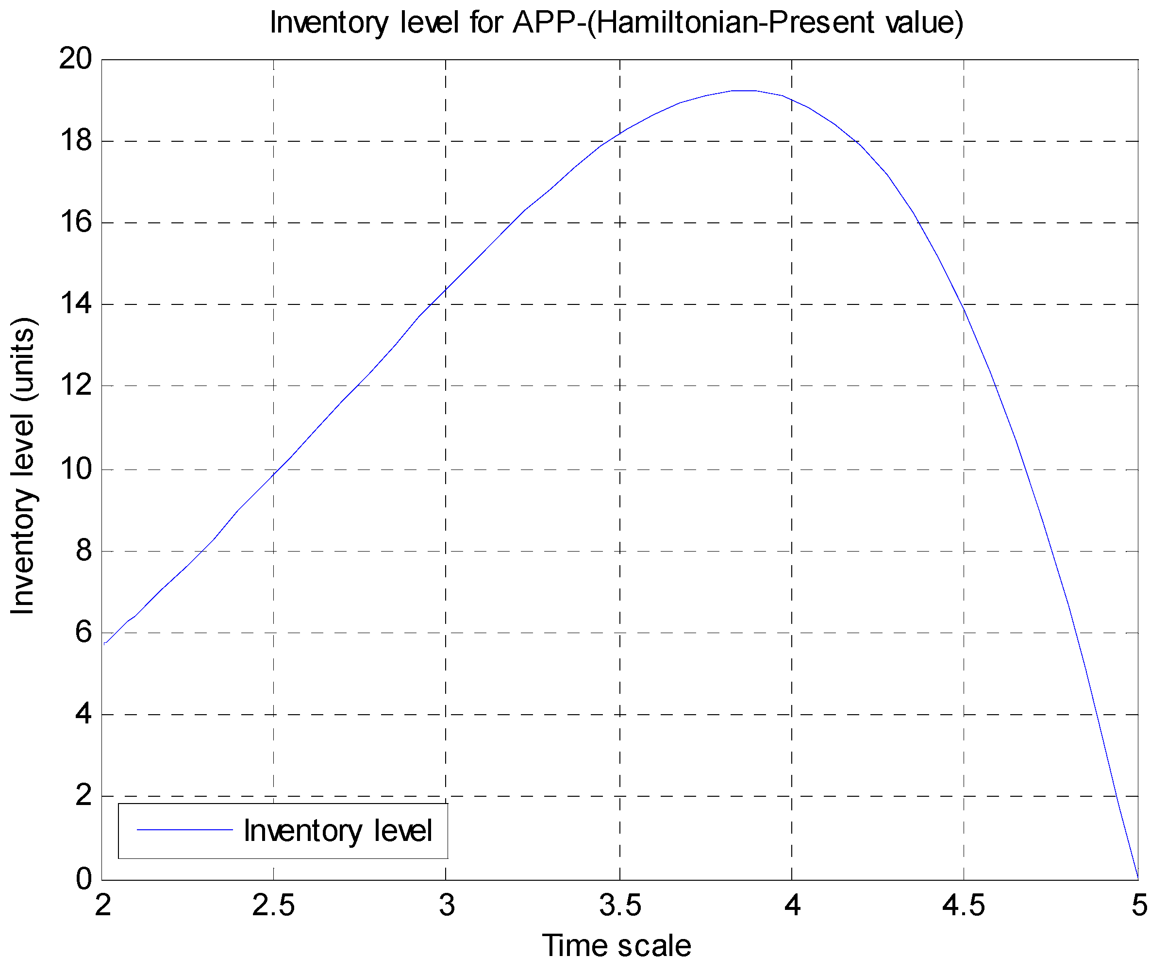
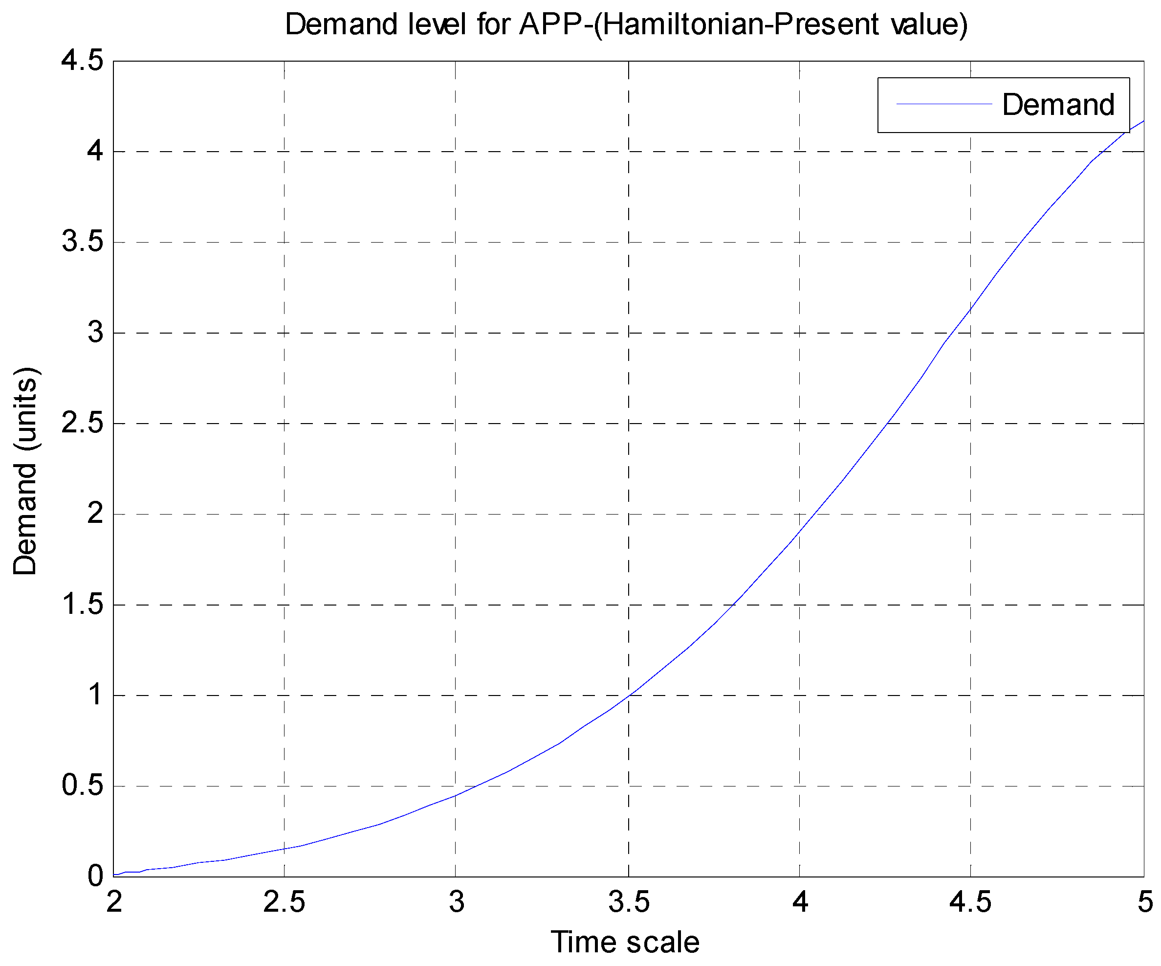
4.2.2. Optimal Control for APP with a Discount Factor: A Hamiltonian “Present Value”

In economics, several problems in OC present a discount factor $e^{-\mathsf{\delta }t}$. In this work, this discount factor is applied to production-inventory systems, as the ratio between the EOQ and Capacity. Based on this, the optimal control problem is of the form:

$$\underset{u\left(t\right)}{\min } J={\displaystyle \underset{t_0}{\overset{t_1}{\int }}W\left(x,u,t\right)e^{-\mathsf{\delta }t}dt}$$

(6a)

$$\text{s.t. }\stackrel{•}{x}=f\left(x,u,t\right),x\left(t_0\right)=x_0,u\left(t\right)\in {\Re }^m$$

(6b)

From where the Hamiltonian is:

$$H\left(x,u,\mathsf{\lambda },t\right)=W\left(x,u,t\right)e^{-\mathsf{\delta }t}+\mathsf{\lambda }f\left(x,u,t\right)$$

(7)

Defining the Hamiltonian “Present value” by:

$$\text{H}=H{e}^{-\mathsf{\delta }t}=W\left(x,u,t\right)+\mathsf{\lambda }{e}^{\mathsf{\delta }t}f\left(x,u,t\right)$$

(8)

Considering the relation: $m\left(t\right)=\mathsf{\lambda }\left(t\right)e^{\mathsf{\delta }t}$, after some manipulation, a detailed discussion is on [55], the Hamiltonian “Present value” is:

$$\text{H}\left(x,u,m,t\right)=G\left(x,u,t\right)+mf\left(x,u,t\right)$$

(9)

The interest is to apply both Optimal Control formulations to the dynamic system from Equations (3) and (4), which results are provided in the following section.

4.2.3. Stability Analysis for APP Problem

Theorem 1. (LaSalle`s Invariance Principle)

Let $f\left(x\right)$ be a locally Lipschitz function defined over a domain $D\subset {\Re }^n$ and $\mathsf{\Omega }\subset D$ be a compact set that is positively invariant with respect to $\stackrel{•}{x}=f\left(x\right)$. Let $V\left(x\right)$ be a continuously differentiable function defined over D such that $\stackrel{•}{V}\left(x\right)\le 0$ in $\mathsf{\Omega }$. Let E be the set of all points in $\mathsf{\Omega }$ where $\stackrel{•}{V}\left(x\right)=0$, and M be the largest invariant set in E. Then every solution starting in $\mathsf{\Omega }$ approaches M as $t\to \infty$.

In order to apply Theorem 1, for stability purposes, in the dynamical system conformed by Equations (3) and (4), the input (demand function) is of the form: $d\left(t\right)=0$. From which, the dynamical system has the form:

$${\stackrel{•}{x}}_1=x_2$$

(10)

$${\stackrel{•}{x}}_2=-\frac{1}{C}\left(x_3-\mathsf{\alpha }\right)x_2-\frac{K}{C}{x}_1$$

(11)

$${\stackrel{•}{x}}_3=\left(1-\frac{\mathsf{\alpha }}{C}\right)x_3+\frac{\mathsf{\alpha }}{C}{x}_1$$

(12)

Considering that: $x_1=P$, $x_2=\stackrel{•}{P}$ and $x_3=\mathsf{\beta }$, with an equilibrium point in $\left(x_1,x_2,x_3\right)=\left(0,0,0\right)$ from Equations (10)–(12). To probe stability, a Lyapunov candidate function is proposed such as:

$$V\left(x_1,x_2,x_3\right)=\frac{1}{2}{\left(x_1-x_3\right)}^2+\frac{1}{2}{x}_2^2$$

(13)

Corollary 2. ([56]) Let x = 0 be an equilibrium point for $\stackrel{•}{x}=f\left(x\right)$. Let $V:D\to R$ be a continuously differentiable positive definite function on a domain D containing the origin x = 0, such that $\stackrel{•}{V}\left(x\right)\le 0$ in D. Let $S=\left\{x\in D|\stackrel{•}{V}\left(x\right)=0\right\}$ and suppose that no solution can stay identically in S, other than the trivial solution. Then, the origin is asymptotically stable. Applying the condition $\stackrel{•}{V}\le 0$ to Equation (13):

$$\stackrel{•}{V}=x_1{\stackrel{•}{x}}_1-x_1{\stackrel{•}{x}}_3-{\stackrel{•}{x}}_1{x}_3+x_3{\stackrel{•}{x}}_3+x_2{\stackrel{•}{x}}_2$$

(14)

After some algebraic manipulation Equation (14) is of the form:

$$\stackrel{•}{V}=\left(x_1-x_3\right)\left[{\stackrel{•}{x}}_1-{\stackrel{•}{x}}_3\right]+x_2{\stackrel{•}{x}}_2$$

(15)

Substituting Equations (10)–(12) in Equation (15):

$$\stackrel{•}{V}=x_1{x}_2-\left(1-\frac{\mathsf{\alpha }}{C}\right)x_1{x}_3-\frac{\mathsf{\alpha }}{C}{x}_1^2-x_2{x}_3+\left(1-\frac{\mathsf{\alpha }}{C}\right)x_3^2+\frac{\mathsf{\alpha }}{C}{x}_1{x}_3-\frac{1}{C}{x}_2^2{x}_3+\frac{\mathsf{\alpha }}{C}{x}_2^2-\frac{K}{C}{x}_1{x}_2$$

(16)

Grouping terms and factorizing in Equation(16):

$$\stackrel{•}{V}=\left(1-\frac{K}{C}\right)x_1{x}_2+\left(\frac{2\mathsf{\alpha }}{C}-1\right)x_1{x}_3-x_2{x}_3-\frac{\mathsf{\alpha }}{C}{x}_1^2+\left(1-\frac{\mathsf{\alpha }}{C}\right)x_3^2-\frac{1}{C}{x}_2^2\left[x_3-\mathsf{\alpha }\right]$$

(17)

The following condition must be satisfied in Equation (17) for stability purposes: $\mathsf{\alpha }=\frac{K}{2}$. From which we have:

$$\stackrel{•}{V}=-\frac{\mathsf{\alpha }}{C}{x}_1^2-\frac{1}{C}{x}_2^2\left[x_3-\mathsf{\alpha }\right]+\left(1-\frac{\mathsf{\alpha }}{C}\right)x_3^2-x_2{x}_3$$

(18)

Considering that $x_1,x_2,x_3>0$ and ${\left|x\right|}^2=\left|x_2\right|\left|x_3\right|$.

$$\stackrel{•}{V}=-\frac{\mathsf{\alpha }}{C}{x}_1^2-\frac{1}{C}{x}_2^2\left[x_3-\mathsf{\alpha }\right]-\left(\frac{\mathsf{\alpha }}{C}-1\right)x_3^2-{\left|x\right|}^2$$

(19)

From Equation (19), in order to satisfy $\stackrel{•}{V}\le 0$, a necessary and sufficient condition is to achieve: $x_3>\mathsf{\alpha }$ with $\mathsf{\alpha }>C.$

5. Results and Discussion

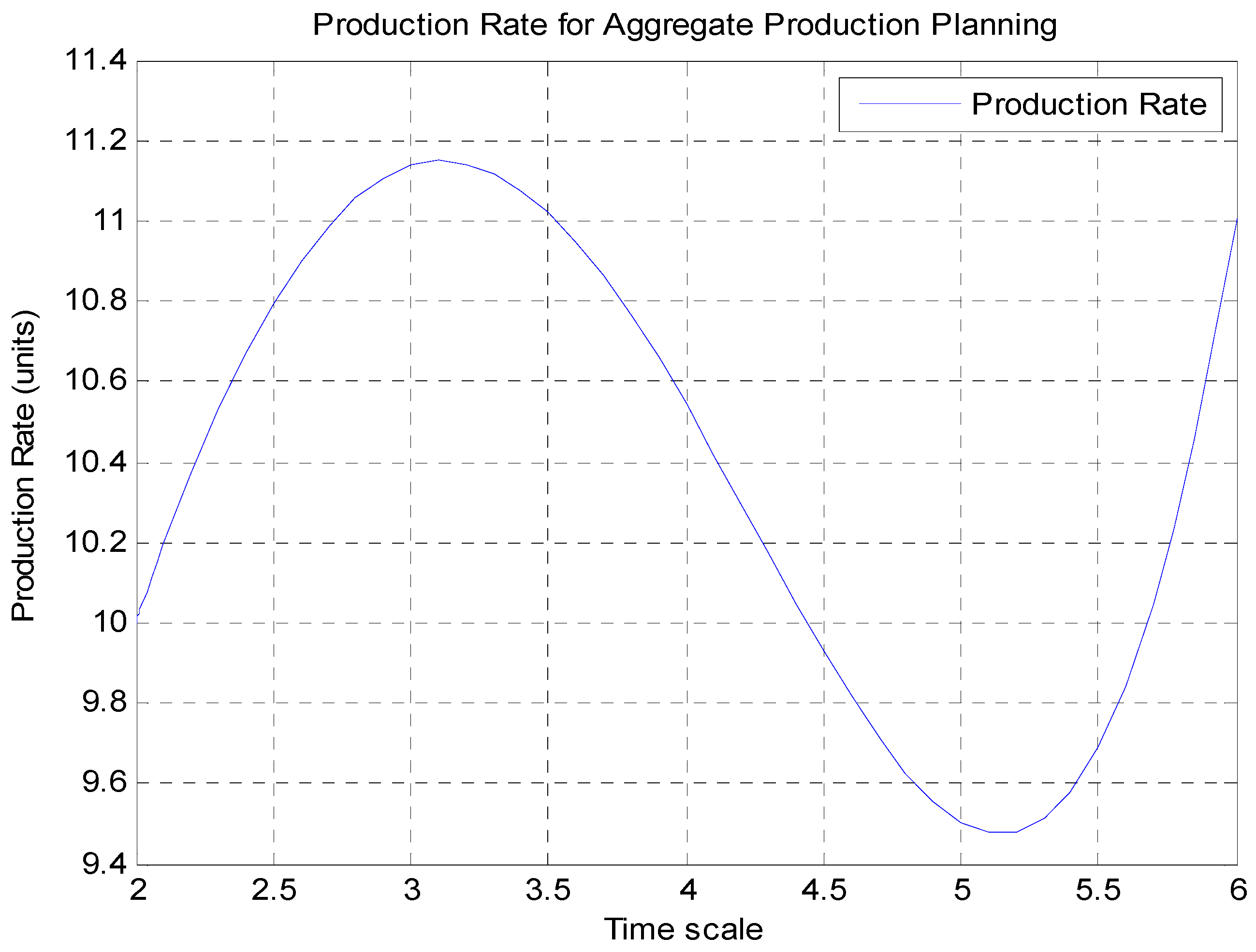
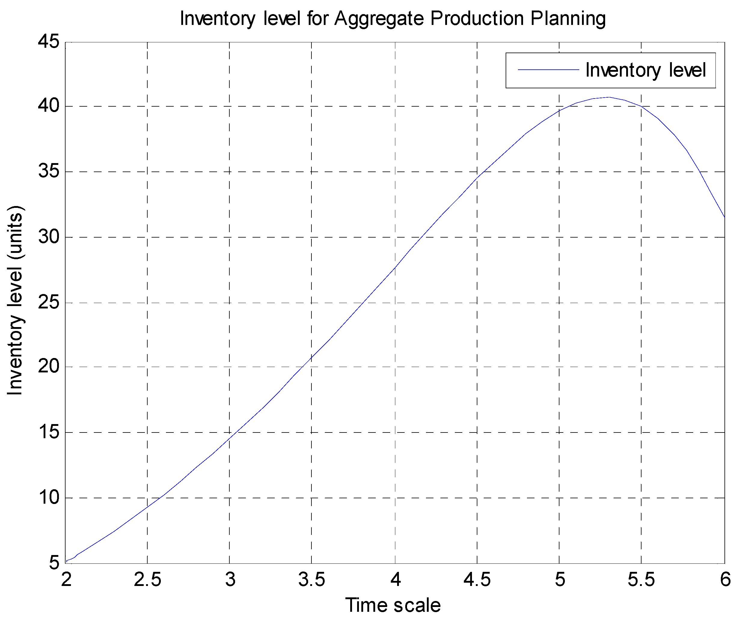
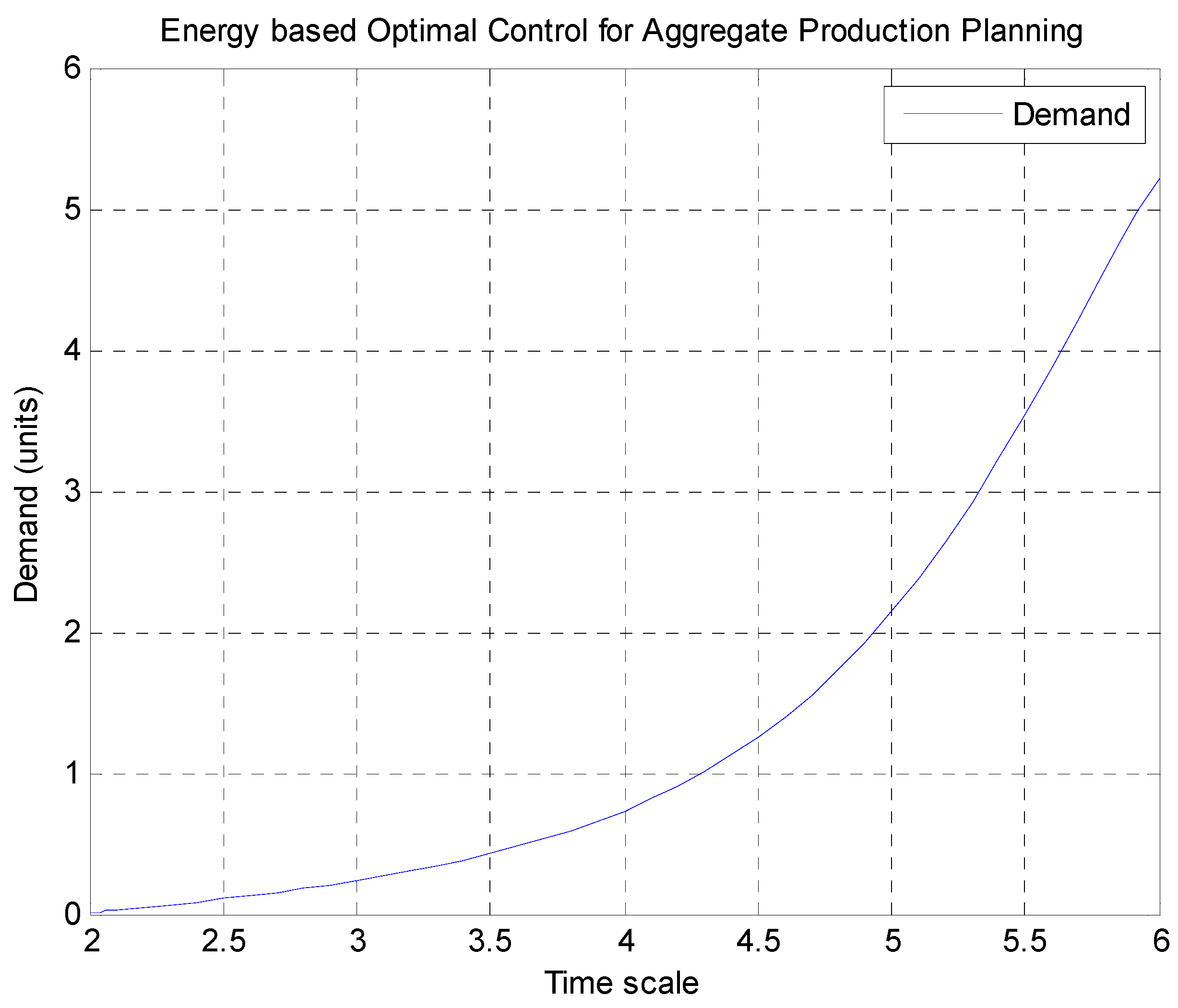
5.1. Energy Based Optimal Control Formulation: Continuous Inventory Policy Approach

Consider the following energy based-Optimal Control problem:

$$\underset{u}{\min }{\displaystyle \underset{o}{\overset{t_f}{\int }}\frac{1}{2}{u}^{2}dt},\text{ s.t. }{\stackrel{•}{x}}_1=x_2$$

(20a)

$${\stackrel{•}{x}}_2=-\left(\frac{x_3-\mathsf{\alpha }}{C}\right)x_2-\frac{K}{C}{x}_1+\frac{1}{C}u,{\stackrel{•}{x}}_3=\left(1-\frac{\mathsf{\alpha }}{C}\right)x_3+\frac{\mathsf{\alpha }}{C}{x}_1-u$$

(20b)

Calculating the Hamiltonian from:

$$H\left(x,u,\mathsf{\lambda },t\right)=F\left(x,u,\mathsf{\lambda },t\right)+\mathsf{\lambda }f\left(x,u,\mathsf{\lambda },t\right)$$

(21)

Applying first condition from Pontryagin Maximum Principle:

$${\stackrel{•}{\mathsf{\lambda }}}_i=-\frac{\partial H}{\partial x_i}$$

(22)

We achieve the following set of ODE, which are the co-states:

$${\stackrel{•}{\mathsf{\lambda }}}_1=\frac{K}{C}{\mathsf{\lambda }}_2-\frac{\mathsf{\alpha }}{C}{\mathsf{\lambda }}_3$$

(23)

$${\stackrel{•}{\mathsf{\lambda }}}_2=-\left({\mathsf{\lambda }}_1-\frac{\left(x_3-\mathsf{\alpha }\right)}{C}{\mathsf{\lambda }}_2\right)$$

(24)

$${\stackrel{•}{\mathsf{\lambda }}}_3=-\left(-\frac{{\mathsf{\lambda }}_2{x}_2}{C}+\left(1-\frac{\mathsf{\alpha }}{C}\right){\mathsf{\lambda }}_3\right)$$

(25)

$$H=\frac{1}{2}{u}^2+{\mathsf{\lambda }}_1{x}_2+{\mathsf{\lambda }}_2\left(-\left(\frac{x_3-\mathsf{\alpha }}{C}\right)x_2-\frac{K}{C}{x}_1+\frac{1}{C}u\right)+{\mathsf{\lambda }}_3\left(\left(1-\frac{\mathsf{\alpha }}{C}\right)x_3+\frac{\mathsf{\alpha }}{C}{x}_1-u\right)$$

(26)

Applying the second condition from Pontryagin Maximum Principle:

$$\frac{\partial H}{\partial u}=u+\frac{{\mathsf{\lambda }}_2^{*}}{C}-{\mathsf{\lambda }}_3^{*}$$

(27)

and $\frac{{\partial }^{2}H}{\partial u^2}=1>0$ thus we have a minimum. Finally, substituting $u={\mathsf{\lambda }}_3^{*}-\frac{{\mathsf{\lambda }}_2^{*}}{C}$ in the set of states and co-states the following simulations are achieved.

In order to present a discussion over the previous results, Figure 1 establishes the production rate behavior over time which has the characteristic of a maximum and minimum level over the horizon presented. Figure 2 presents a maximum level in the same time horizon this is based on the formulation of the first order differential equation which characterizes it. Figure 3 relates that the demand level increase conforms with the time horizon increases.

Figure 1. Production Rate for APP (time scale in days).

Figure 1. Production Rate for APP (time scale in days).

Figure 2. Inventory level for APP (time scale in days).

Figure 2. Inventory level for APP (time scale in days).

Figure 3. Demand level for APP (time scale in days).

Figure 3. Demand level for APP (time scale in days).

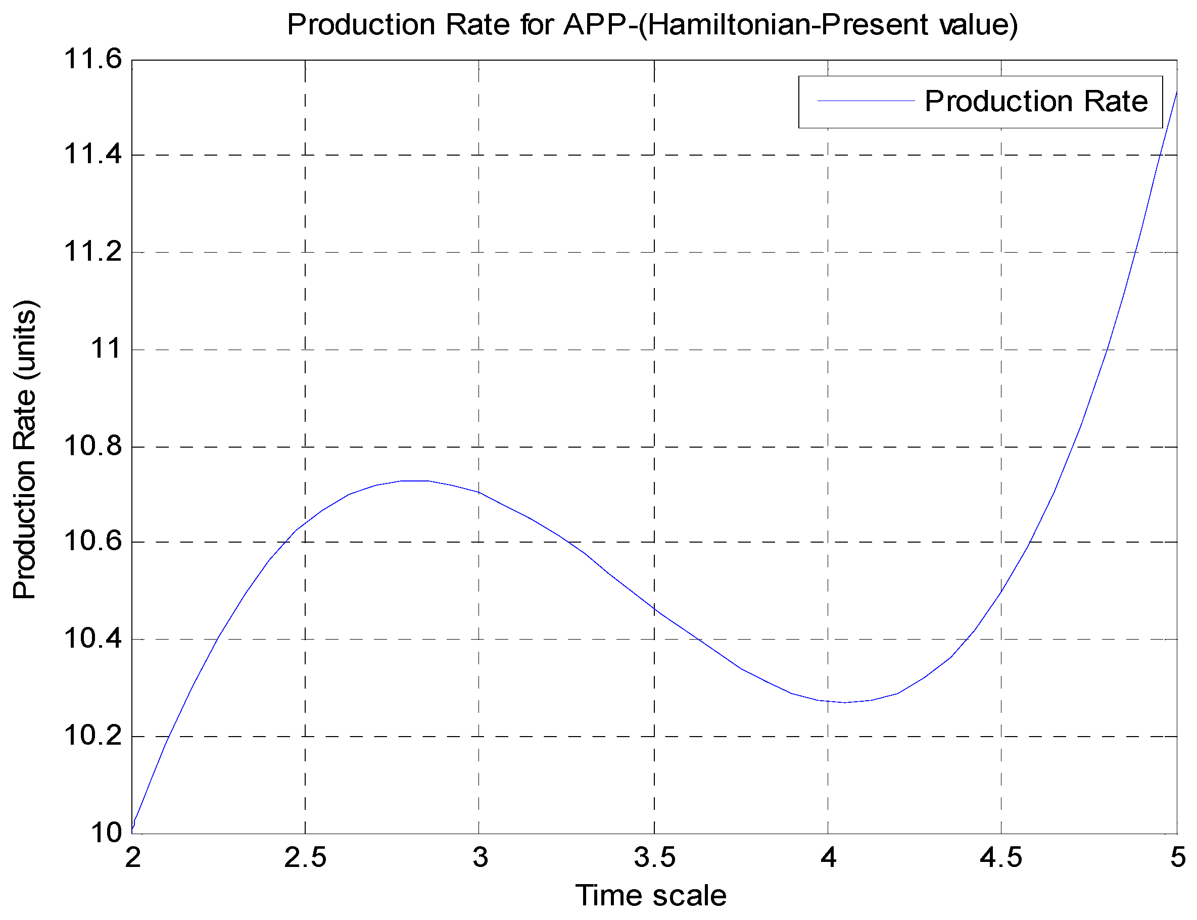
5.2. Energy Based-Optimal Control with a Discount Factor: A Hamiltonian “Present Value”

Based on a previous work, in [57] which applies a discount factor in the performance index, this approach considers the following problem with a discount factor

$$\underset{u}{\min }{\displaystyle \underset{o}{\overset{t_f}{\int }}\frac{1}{2}\left(u^2+x_1^2\right)e^{-\left(\frac{\mathsf{\alpha }}{C}\right)t}dt},\text{ s.t. }{\stackrel{•}{x}}_1=x_2$$

(28a)

$${\stackrel{•}{x}}_2=-\left(\frac{x_3-\mathsf{\alpha }}{C}\right)x_2-\frac{K}{C}{x}_1+\frac{1}{C}u,{\stackrel{•}{x}}_3=\left(1-\frac{\mathsf{\alpha }}{C}\right)x_3+\frac{\mathsf{\alpha }}{C}{x}_1-u$$

(28b)

The first condition for the Hamiltonian-Present value, which are the co-states:

$$\stackrel{•}{m}=-\frac{\partial H}{\partial x}+\left(\frac{\mathsf{\alpha }}{C}\right)m$$

(29)

where the Hamiltonian as the form:

$$H=\frac{1}{2}\left(x_1^2+u^2\right)+m_1{x}_2+m_2\left(-\left(\frac{x_3-\mathsf{\alpha }}{C}\right)x_2-\frac{K}{C}{x}_1+\frac{1}{C}u\right)+m_3\left(\left(1-\frac{\mathsf{\alpha }}{C}\right)x_3+\frac{\mathsf{\alpha }}{C}{x}_1-u\right)$$

(30)

The following set of ODE, are for the co-states:

$${\stackrel{•}{m}}_1=x_1+\frac{K}{C}{m}_2+\frac{\mathsf{\alpha }}{C}{m}_3+\frac{\mathsf{\alpha }}{C}{m}_1$$

(31)

$${\stackrel{•}{m}}_2=-\left(m_1-\frac{\left(x_3-\mathsf{\alpha }\right)}{C}{m}_2\right)+\frac{\mathsf{\alpha }}{C}{m}_2$$

(32)

$${\stackrel{•}{m}}_3=-\left(-\frac{m_2{x}_2}{C}+\left(1-\frac{\mathsf{\alpha }}{C}\right)m_3\right)+\frac{\mathsf{\alpha }}{C}{m}_3$$

(33)

Applying the second condition from Pontryagin Maximum Principle:

$$\frac{\partial H}{\partial u}=u+\frac{m_2^{*}}{C}-m_3^{*}$$

(34)

and $\frac{{\partial }^{2}H}{\partial u^2}=1>0$ thus we have a minimum. Substituting $u=m_3^{*}-\frac{m_2^{*}}{C}$ in the set of states and co-states, after some manipulation, the following simulations are achieved.

The introduction of the Hamiltonian present value produces a lower a higher production rate level in the dynamics, based on Figure 4 and a lower inventory level (almost half of the energy based inventory level from Section 5.1) which is present in Figure 5. Finally, the demand level increases conform with time horizon increases as is shown in Figure 6.

Figure 4. Production rate for APP (Hamiltonian-present value, time scale in days).

Figure 4. Production rate for APP (Hamiltonian-present value, time scale in days).

Figure 5. Inventory level for APP (Hamiltonian-present value, time scale in days).

Figure 5. Inventory level for APP (Hamiltonian-present value, time scale in days).

Figure 6. Demand level for APP (Hamiltonian-present value, time scale in days).

Figure 6. Demand level for APP (Hamiltonian-present value, time scale in days).

6. Conclusions

This research work presents an Optimal Control formulation for APP problems via the approach of Energy-Based and Hamiltonian-Present value. Stability analysis via LaSalle invariance principle establishes a condition in the inventory level which considers the EOQ parameter. The main contribution of this paper is the mathematical model which integrates a second order dynamical system coupled with a first order dynamical system which incorporates production rate, inventory level, and capacity as well with the associated cost of the work force in the same formulation.

Simulations show conforming with the increased production rate, inventory level achieves a maximum level when that demand level grows. A novel result in relation with the Hamiltonian-present value in the Optimal Control formulation is that it reduces the inventory level compared with the pure energy based approach for APP. Simulations show conforming with the increased production rate, inventory level achieves a maximum level when that demand level grows.

Further work presents the idea of integrating the associated cost with dynamics, and to extend the case studies in the cost functional. Also the interest is to extend the mathematical model, in discrete formulation, to apply Model Predictive Control (MPC). Future research will consider the use of robust optimal control, another way of dealing with uncertainty, where a deterministic uncertain-but-bounded quantity is used (i.e., future demand can be bounded between lower and upper limits, without needing to define the probability of occurrence of each possible event within these limits), and the constraints regarding the operation of the system. Our intention is to extend this work with the application of MPC strategies via a suitable dynamic system which integrates dynamics in the inventory level. A practical real life problem which addresses this approach is our interest as well.

References

1. Moreno, M.S.; Montagna, J.M. A multiperiod model for production planning and design in a multiproduct batch environment. Math. Comput. Model. 2009, 49, 1372–1385. [Google Scholar] [CrossRef]
2. Holt, J.A. PDF versus LP: An empirical aggregate planning comparison. J. Oper. Manag. 1983, 3, 141–147. [Google Scholar] [CrossRef]
3. Foote, B.L.; Ravlndran, A.; Lashine, S. Computational feasibility of multi-criteria models of production, planning and scheduling. J. Comput. Ind. Eng. 1988, 15, 129–138. [Google Scholar] [CrossRef]
4. Buxey, G. Strategy not tactics drives aggregate planning. Int. J. Prod. Econ. 2003, 85, 331–346. [Google Scholar] [CrossRef]
5. Buxey, G. Aggregate planning for seasonal demand: Reconciling theory with practice. Int. J. Oper. Prod. Manag. 2005, 25, 1083–1100. [Google Scholar] [CrossRef]
6. Taubert, W.H. A search decision rule for the aggregate scheduling problem. Manag. Sci. 1968, 14, 343–359. [Google Scholar] [CrossRef]
7. Schroeder, R.G.; Larson, P.D. A Reformulation of the aggregate planning problem. J. Oper. Manag. 1986, 6, 245–256. [Google Scholar] [CrossRef]
8. Nam, S.; Logendram, R. Modified production switching heuristics for aggregate production planning. Comput. Oper. Res. 1995, 22, 531–541. [Google Scholar] [CrossRef]
9. Da Silva, C.G.; Figueira, J.; Lisboa, J.; Barman, S. An interactive decision support system for an aggregate production planning model based on multiple criteria mixed integer linear programming. Omega 2006, 34, 167–177. [Google Scholar] [CrossRef]
10. Buxey, G. Production Planning Under Seasonal Demand: A Case Study Perspective. Omega 1988, 16, 447–455. [Google Scholar] [CrossRef]
11. Wang, R.C.; Liang, T.F. Applying possibilistic linear programming to aggregate production planning. Int. J. Prod. Econ. 2005, 98, 328–341. [Google Scholar] [CrossRef]
12. Tadei, R.; Trubian, J.L.; Avendaño, F.; Croce, D.; Menga, G. Aggregate planning and scheduling in the food industry: A case study. Eur. J. Oper. Res. 1995, 87, 564–573. [Google Scholar] [CrossRef]
13. Gansterer, M. Aggregate planning and forecasting in make-to-order production systems. Int. J. Prod. Econ. 2015, 170, 521–528. [Google Scholar] [CrossRef]
14. Leung, S.C.H.; Wu, Y.; Lai, K.K. Multi-site aggregate production planning with multiple objectives: A goal programming approach. Prod. Plan. Control 2003, 14, 425–436. [Google Scholar] [CrossRef]
15. Chien, Y.I.; Cunningham, W.J. Incorporating production planning in business planning: A linked spreadsheet approach. Prod. Plan. Control 2000, 11, 299–307. [Google Scholar] [CrossRef]
16. Al-e-hashem, S.M.J.; Malekly, H.; Aryanezhad, M.B. A multi-objective robust optimization model for multi-product multi-site aggregate production planning in a supply chain under uncertainty. Int. J. Prod. Econ. 2011, 134, 28–42. [Google Scholar] [CrossRef]
17. Wang, R.C.; Fang, H.H. Aggregate production planning with multiple objectives in a fuzzy environment. Eur. J. Oper. Res. 2001, 133, 521–536. [Google Scholar] [CrossRef]
18. Tang, J.; Wang, D.; Fung, R. Fuzzy formulation for multi-product aggregate production planning. Prod. Plan. Control 2000, 11, 670–676. [Google Scholar] [CrossRef]
19. Fahimnia, B.; Luong, L.; Marian, R. Genetic algorithm optimization of an integrated aggregate production-distribution plan in supply chains. Int. J. Prod. Res. 2012, 50, 81–96. [Google Scholar] [CrossRef]
20. Sillekens, T.; Koberstein, A.; Suhl, L. Aggregate production planning in the automotive industry with special consideration of workforce flexibility. Int. J. Prod. Res. 2011, 49, 5055–5078. [Google Scholar] [CrossRef]
21. Kim, B.; Kim, S. Extended model for a hybrid production planning approach. Int. J. Prod. Econ. 2001, 73, 165–173. [Google Scholar] [CrossRef]
22. Leung, S.C.H.; Chan, S.S.W. A goal programming model for aggregate production planning with resource utilization constraint. Comput. Ind. Eng. 2009, 56, 1053–1064. [Google Scholar] [CrossRef]
23. Mula, J.; Poler, R.; García-Sabater, J.P.; Lario, F.C. Models for production planning under uncertainty: A review. Int. J. Prod. Econ. 2006, 103, 271–285. [Google Scholar] [CrossRef]
24. Bushuev, M. Convex optimization for aggregate production planning. Int. J. Prod. Res. 2014, 52, 1050–1058. [Google Scholar] [CrossRef]
25. García, J.P.; Maheut, J.; García, J. A decision support system for aggregate production planning based on MILP: A case study from the automative industry. In Proceedings of the International Conference on Computers & Industrial Engineering (CIE), Troyes, France, 6–9 July 2009; pp. 366–371.
26. Tavakkoli, R.; Safaei, N. An evolutionary algorithm for a single-item resource-constrained Aggregate Production Planning problem. In Proceedings of the IEEE International Conference on Evolutionary Computation, Vancouver, BC, Canada, 16–21 July 2006; pp. 2851–2858.
27. Vergin, R.C. Production scheduling under seasonal demand. J. Ind. Eng. 1966, 17, 260–266. [Google Scholar]
28. Das, S.K.; Sarin, S.C. An integrated approach to solving the master aggregate scheduling problem. Int. J. Prod. Econ. 1994, 34, 167–178. [Google Scholar] [CrossRef]
29. Wienke, M. Aggegate Models for Transient Production Planning. Ph.D. Thesis, Arizona State University, Tempe, AZ, USA, 2015. [Google Scholar]
30. Disney, S.M.; Naim, M.M.; Towill, D.R. Dynamic simulation modelling for lean logistics. Int. J. Phys. Distrib. Logist. Manag. 1997, 27, 174–196. [Google Scholar] [CrossRef]
31. Disney, S.M.; Naim, M.M.; Towill, D.R. Genetic algorithm optimization of a class of inventory control system. Int. J. Prod. Econ. 2000, 68, 259–278. [Google Scholar] [CrossRef]
32. Dejonckheere, J.; Disney, S.M.; Lambrecht, M.R.; Towill, D.R. Measuring and avoiding the bullwhip effect: A control theoretic approach. Eur. J. Oper. Res. 2003, 147, 567–590. [Google Scholar] [CrossRef]
33. Tang, O.; Naim, M.M. The impact of information transparency on the dynamic behavior of a hybrid manufacturing/remanufacturing system. Int. J. Prod. Res. 2004, 42, 4135–4152. [Google Scholar] [CrossRef]
34. Disney, S.M.; Towill, D.R. A discrete transfer function model to determine the dynamic stability of a vendor managed inventory supply chain. Int. J. Prod. Res. 2002, 40, 179–204. [Google Scholar] [CrossRef]
35. Axsater, S. Control theory concepts in production and inventory control. Int. J. Syst. Sci. 1985, 16, 161–169. [Google Scholar] [CrossRef]
36. Edghill, J.S.; Towill, D.R. The use of systems dynamics in manufacturing systems. Trans. Inst. Meas. Control 1989, 11, 208–216. [Google Scholar] [CrossRef]
37. Riddalls, C.E.; Bennett, S. The stability of supply chains. Int. J. Prod. Res. 2002, 40, 459–475. [Google Scholar] [CrossRef]
38. Ortega, M.; Lin, L. Control theory applications to the production–inventory problem: A review. Int. J. Prod. Res. 2004, 42, 2303–2322. [Google Scholar] [CrossRef]
39. Dejonckheere, J.; Disney, S.M.; Lambrecht, M.R.; Towill, D.R. The impact of information enrichment on the Bullwhip effect in supply chains: A control engineering perspective. Eur. J. Oper. Res. 2004, 153, 727–750. [Google Scholar] [CrossRef]
40. Sterman, J. Business Dynamics: Systems Thinking and Modeling for a Complex World; McGraw-Hill: New York, NY, USA, 2000. [Google Scholar]
41. Dejonckheere, J.; Disneys, S.M.; Lambrecht, M.; Towill, D.R. The dynamics of aggregate planning. Prod. Plan. Control 2003, 14, 497–516. [Google Scholar] [CrossRef]
42. Bijulal, D.; Venkateswaran, J.; Hemachandra, N. Service levels, system cost and stability of production-inventory control systems. Int. J. Prod. Res. 2011, 49, 7085–7105. [Google Scholar] [CrossRef]
43. Riddalls, C.E.; Bennett, S. Production-inventory system controller design and supply chain dynamics. Int. J. Syst. Sci. 2002, 33, 181–195. [Google Scholar] [CrossRef]
44. Poles, R. System Dynamics modeling of a production and inventory system for remanufacturing to evaluate system improvement strategies. Int. J. Prod. Econ. 2013, 144, 189–199. [Google Scholar] [CrossRef]
45. Mason-Jones, R.; Towill, D.R. Using the Information Decoupling Point to Improve Supply Chain Performance. Int. J. Logist. Manag. 1999, 10, 13–26. [Google Scholar] [CrossRef]
46. Chandra, C.; Grabis, J. Application of multi-steps forecasting for restraining the bullwhip effect and improving inventory performance under autoregressive demand. Eur. J. Oper. Res. 2005, 166, 337–350. [Google Scholar] [CrossRef]
47. Agrawal, S.; Sengupta, R.N.; Shanker, K. Impact of information sharing and lead time on bullwhip effect and on-hand inventory. Eur. J. Oper. Res. 2009, 192, 576–593. [Google Scholar] [CrossRef]
48. Costantino, F.; di Gravio, G.; Shaban, A.; Tronci, M. Exploring the bullwhip effect and inventory stability in a seasonal supply chain. Int. J. Eng. Bus. Manag. 2013. [Google Scholar] [CrossRef]
49. Naim, M.M.; Wikner, J.; Grubbström, R.W. A net present value assessment of make-to-order and make-to-stock manufacturing systems. Omega 2007, 35, 524–532. [Google Scholar] [CrossRef]
50. Disney, S.M.; Towill, D.R. A procedure for the optimization of the dynamic response of a Vendor Managed Inventory system. Comput. Ind. Eng. 2002, 43, 27–58. [Google Scholar] [CrossRef]
51. Davizón, Y.A.; Soto, R.; Rodríguez, J.J.; Rodríguez-Leal, E.; Martínez-Olvera, C.; Hinojosa, C. Demand Management Based on Model Predictive Control Techniques. Math. Prob. Eng. 2014. [Google Scholar] [CrossRef]
52. Zanwar, D.R.; Deshpande, V.S.; Modak, J.P.; Gupta, M.M.; Agrawal, K.N. Determination of mass, damping coefficient, and stiffness of production system using convolution integral. Int. J. Prod. Res. 2015, 53, 4351–4362. [Google Scholar] [CrossRef]
53. Warburton, R.D.H.; Hodgson, J.P.E.; Nielsen, E.H. Exact solutions to the supply chain equations for arbitrary time-dependent demands. Int. J. Prod. Econ. 2014, 151, 195–205. [Google Scholar] [CrossRef]
54. Kirk, D.E. Optimal Control Theory: An Introduction; Dover Publications: Mineola, NY, USA, 2004. [Google Scholar]
55. Cerdá, E. Dynamic Optimization; Alfaomega: Madrid, Spain, 2012. (In Spanish) [Google Scholar]
56. Khalil, H.K. Nonlinear Systems; Prentice Hall: Jamestown, ND, USA, 2002. [Google Scholar]
57. Feng, L.; Zhang, J.; Tang, W. Optimal Inventory Control and pricing of Perishable items without shortages. IEEE Trans. Autom. Sci. Eng. 2015. [Google Scholar] [CrossRef]