Article

Robust Sliding Mode Control of Permanent Magnet Synchronous Generator-Based Wind Energy Conversion Systems

1
Department of Computer Science, Taiyuan Normal University, Taiyuan 030619, Shanxi, China
2
Department of Electrical and Computer Engineering, Southern Illinois University, Edwardsville, IL 62026, USA
*
Author to whom correspondence should be addressed.
Current address: Basler Electric Co., 12570 IL-143, Highland, IL 62249, USA
These authors contributed equally to this work.
Sustainability 2016, 8(12), 1265; https://doi.org/10.3390/su8121265
Submission received: 17 September 2016 / Revised: 19 November 2016 / Accepted: 30 November 2016 / Published: 5 December 2016
(This article belongs to the Special Issue Sustainable Electric Power Systems Research)

Abstract

:
The subject of this paper pertains to sliding mode control and its application in nonlinear electrical power systems as seen in wind energy conversion systems. Due to the robustness in dealing with unmodeled system dynamics, sliding mode control has been widely used in electrical power system applications. This paper presents first and high order sliding mode control schemes for permanent magnet synchronous generator-based wind energy conversion systems. The application of these methods for control using dynamic models of the d-axis and q-axis currents, as well as those of the high speed shaft rotational speed show a high level of efficiency in power extraction from a varying wind resource. Computer simulation results have shown the efficacy of the proposed sliding mode control approaches.

1. Introduction

Concerns over the environmental impacts and scarcity of fossil fuels have led to increased usage and growing demand of alternative energy resources, such as wind and solar energy. Studies predict 20% of the United State’s electrical energy will come from wind by 2030 [1]. Modern wind energy conversion systems (WECS) are designed to maximize the electrical power extraction from wind input, which is commonly known as the maximum power point tracking (MPPT) [2,3,4]. Due to the highly unpredictable nature of wind, the ability to obtain satisfactory efficiency has been difficult until recent advances in nonlinear control technologies [5].
In recent years, as WECS have moved away from the doubly-fed induction generators (DFIGs) and more towards permanent magnet synchronous generators (PMSGs), even further emphasis has been placed on efficient control strategies due to the high price and complexity of typical aerodynamic control systems [6]. Using PMSGs over DFIGs renders higher reliability, greater efficiency, a larger energy to weight ratio and an improved power factor to wind energy conversion systems (WECS) [7,8]. A PMSG eliminates the necessity of the gearbox, which further reduces costs associated with maintenance by allowing for direct coupling of the shafts of the generator and the turbine [9].
One proposed control method that shows promise in helping to achieve high efficiency, robustness and stability is sliding mode control (SMC). For WECS employing DFIGs, SMC applied to torque control demonstrates high MPPT with low variations in torque. The usefulness of this control method extends into synchronous machines, as well. Research into the use of SMC in PMSGs effectively demonstrates the potential power of this control method. The strength of SMC comes from the ability to control high-order systems, while exhibiting resiliency against disturbances and variations in model parameters. Research into SMC for PMSGs illustrates the potential of this control method and accentuates SMCs promise as a candidate for achieving the goal of increasing the efficiency level in regards to MPPT. Results demonstrated by research involving the use of SMC with permanent magnet synchronous motors (PMSMs) and permanent magnet synchronous generators (PMSGs) continue to demonstrate the strength of SMC as a viable method for effective control of synchronous machines [10,11,12,13,14].
Although the positive attributes of SMC make it seem an ideal control method, it does not exist without fault. The phenomenon in first-order sliding mode control, known as chattering, invites an understandable level of criticism. Due to the non-idealities in switching devices, the response of the system under SMC oscillates about the desired reference, known as the sliding surface. This leads to higher mechanical wear, lower accuracy and heat loss in power circuits. Modifications in the first-order sliding mode control calculation to assume imperfect switching times, such as using hysteresis instead of signum functions, can be utilized in order to compensate for chattering, but such methods complicate calculations for a relatively small reduction in chattering [15,16,17,18]. Thus, the principal method for avoiding chattering is to increase the order of sliding mode control by forcing higher order derivatives of the sliding manifold to zero [19,20,21]. In an ideal case, careful usage of high order sliding mode control removes chattering as a concern [22,23,24]. Advances in generalizing the sliding mode control to these higher orders have allowed the system to maintain high accuracy and robustness while still reducing the effect of chattering [25,26,27].
The structure of this paper is as follows: Section 2 develops and outlines models for the aerodynamics of the wind turbine and the PMSG. Section 3 presents the design of first- and high order sliding mode control methods for PMSG-based WECS. Section 4 gives the results comparison based on the simulations conducted in MATLAB and SIMULINK. Lastly, Section 5 concludes this work with comments on the effectiveness of the proposed control methods.

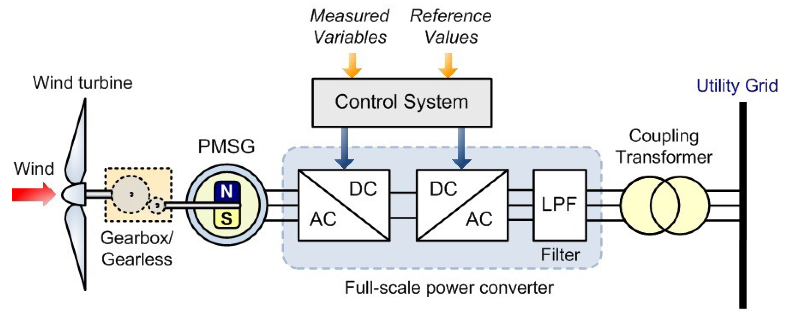
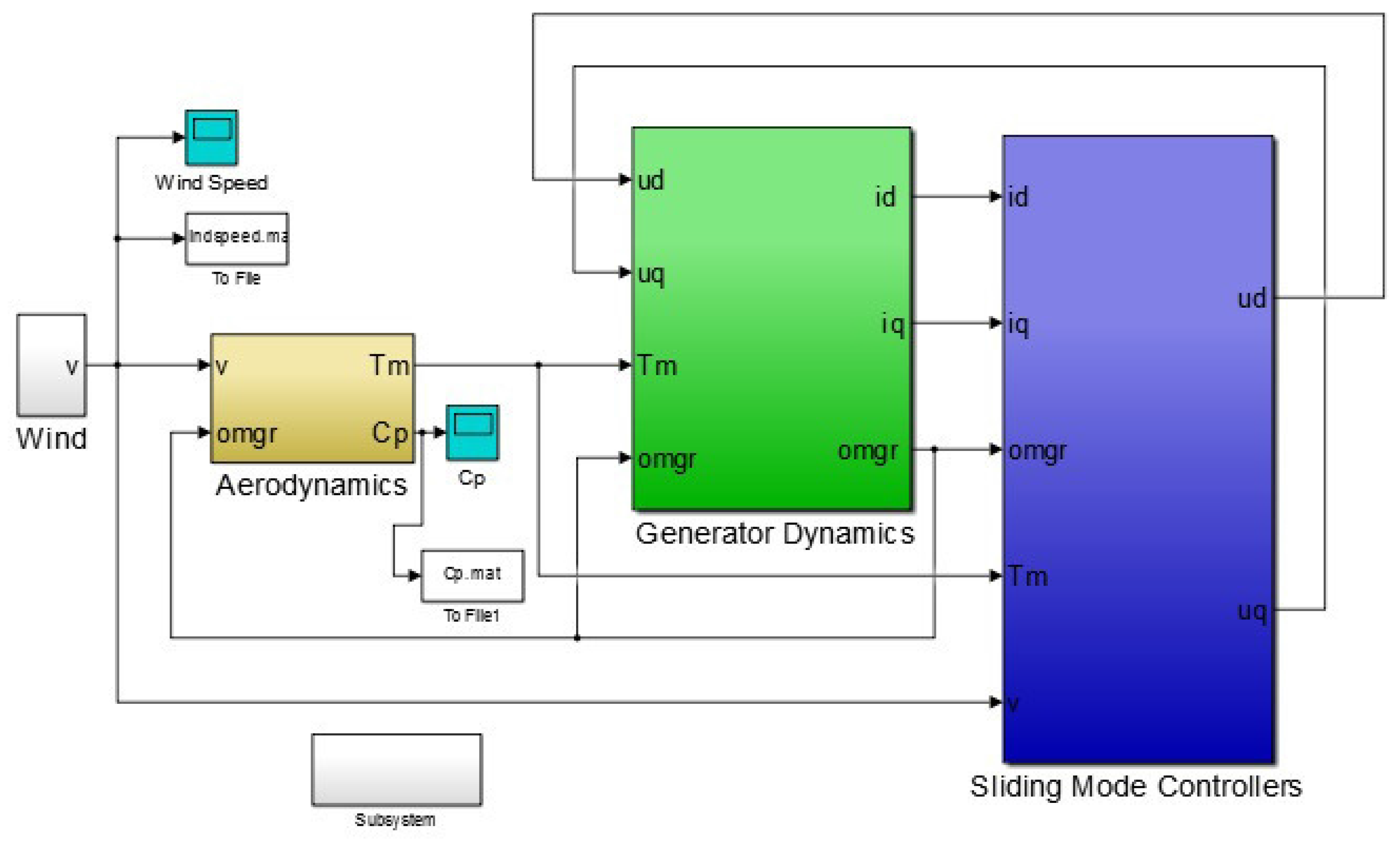
2. Wind Energy Conversion PMSG Model

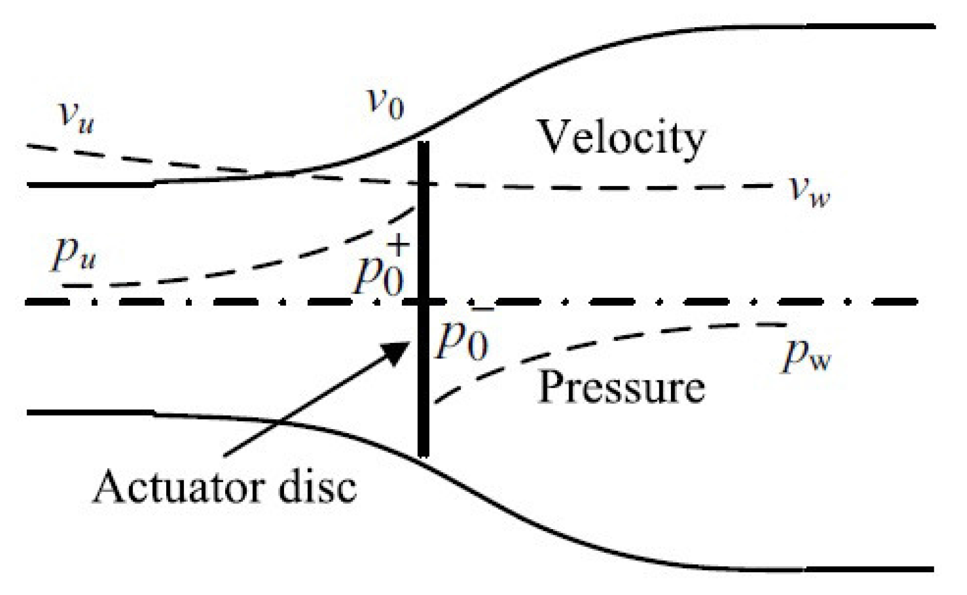
2.1. Ideal Actuator Disk Model

The aerodynamic behavior of an ideal wind turbine is modeled through an actuator disk used to extract mechanical power from the dynamic wind power input. Figure 1 shows the actuator disk model, where the variables with subscript u indicate conditions (velocity, pressure) in front of the disk, subscript 0 indicates conditions at the disk and subscript w indicates conditions behind the disk.
Wind of air mass m, pressure p, density ρ and velocity v transfers momentum H = m ( v u - v w ) to a disk of cross-sectional area A. The resulting force is:
F = Δ H Δ t = Δ m ( v u - v w ) Δ t = ρ A v 0 ( v u - v w )
Equivalently, the force on the actuator disk can be written as:
F = A ( p 0 + - p 0 - )
Based on Bernoulli’s equation, the pressure difference is:
( p 0 + - p 0 - ) = 1 2 ρ ( v u 2 - v w 2 )
which means the force can be expressed as:
F = 1 2 ρ A ( v u 2 - v w 2 )
From Equations (1)–(4), the wind velocity at the actuator disk can be found in terms of input and output wind speed in the form of:
v 0 = 1 2 ( v u + v w )
Equivalently, we have:
v u - v w = 2 ( v u - v 0 )
The kinetic energy of the air mass traveling at speed v is E = 1 2 m v 2 . Since air mass, which passes the actuator disk in 1 s of time, can be expressed as m = ρ A v 0 , where A is the cross-sectional area, the input wind power is given in the form:
P w i n d = 1 2 ρ A v 0 3
The power extracted by the actuator disk, i.e., the power supplied to the rotor (turbine), can be obtained as:
P r o t o r = 1 2 ρ A v 0 ( v u 2 - v w 2 ) = 1 2 ρ A v 0 3 4 a ( 1 - a ) 2
where:
a = 1 - v 0 v u
Denote the power coefficient C p as the power ratio of power extracted by the actuator disk to the power input from wind. C p can be obtained as:
C p = P r o t o r P w i n d = 4 a ( 1 - a ) 2
From Equation (10), C p achieves its maximum value C p , m a x = 0.59 , when a = 1 3 , known as the Betz limit, and represents the maximum power extraction of a wind energy conversion system in the most optimal case.

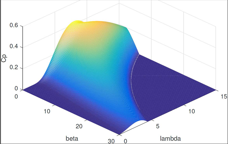
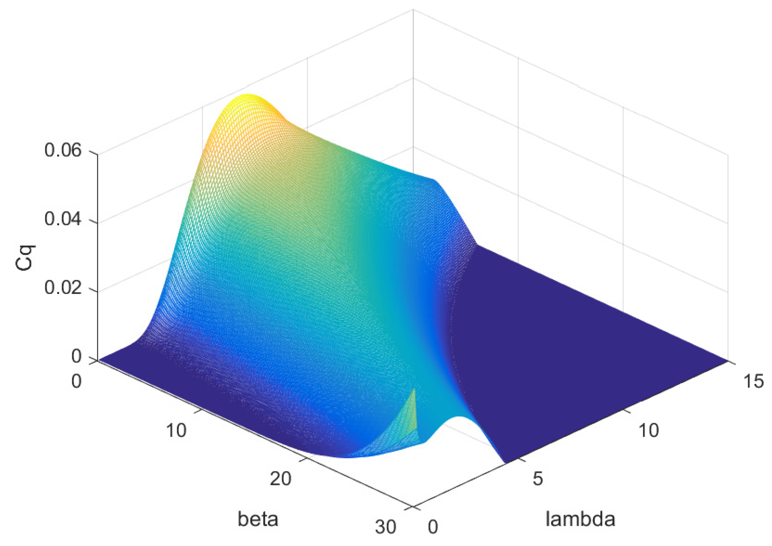
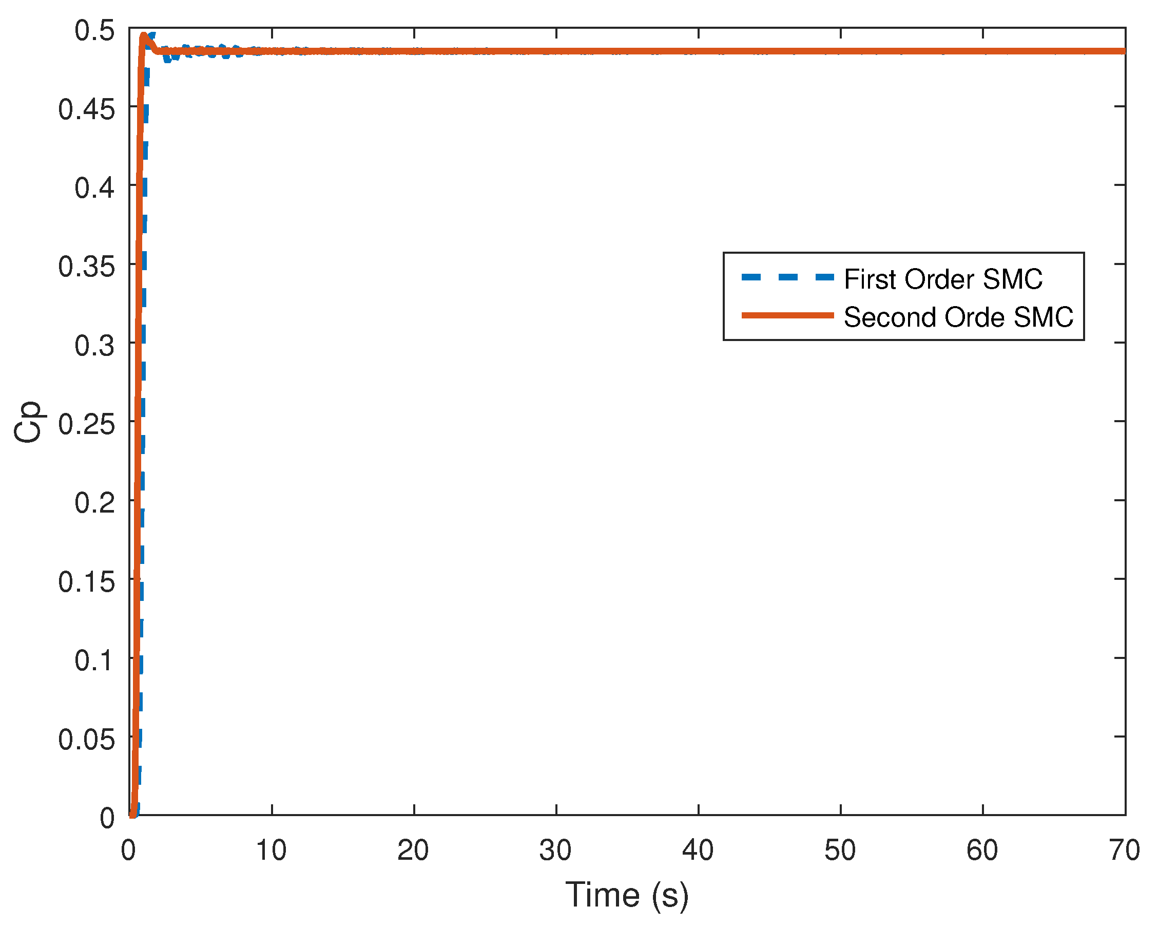
2.2. Performance of a Non-Ideal Wind Turbine

For most practical wind energy conversion systems (WECS), as shown in Figure 2, the maximum achievable power extraction is approximately 70%–80% of the Betz limit (41.5%–47.4% in total efficiency from power extraction from wind) [29,30].
C p = P r o t o r P w i n d < 0.5
Denote the tip speed ratio λ as the ratio between the peripheral blade speed and the corresponding wind speed v (Note: v = v 0 ) as:
λ = ω r o t o r R t v
where R t is the blade length of the turbine.
The C p power coefficient describes the power extraction efficiency of a wind turbine. A commonly-used C p power coefficient is calculated as a function of the tip speed ratio λ and the blade pitch β and is given by the following mathematical approximation [31,32]:
C p ( λ , β ) = c 1 ( c 2 λ i - c 3 β - c 4 ) e - c 5 λ i
λ i = ( 1 λ + c 6 β - c 7 β 3 + 1 ) - 1
where c 1 c 7 are wind turbine constants. Consider β = 0 o , c 1 = 0.39 , c 2 = 116 , c 3 = 0.4 , c 4 = 5 , c 5 = 16.5 , c 6 = 0.089 and c 7 = 0.035 ; we have C p , m a x = 0.4953 , and the optimal tip speed ratio λ o = 7.2 , which falls within the range of realistic expectations for a wind turbine. The power coefficient C p curve is shown in Figure 3.
The torque at the rotor can be expressed in the form as:
τ r o t o r = P r o t o r ω r o t o r = 1 2 ρ C p π R t 2 v 3 ω r o t o r
where R t is the blade length of the turbine and v is the wind speed.
For torque assessment and control purposes, the torque coefficient C q , which characterizes the rotor output torque, is derived from the power coefficient simply dividing it by the tip speed ratio as:
C q = C p λ
The resultant C q curve is shown in Figure 4.

2.3. Permanent Magnet Synchronous Generator Model

Park’s transform is used to transfer the a b c coordinate frame permanent magnet synchronous generator model to the d q coordinate frame model. This yields the following equations for the direct and quadrature axis voltages:
u d = - R s i d - L d d i d d t + L q i q ω e
u q = - R s i q - L q d i q d t + ( - L d i d + Ψ m ) ω e
For a surface-mounted PMSG, L d = L q , which we hereby denote as L for both quantities. Rearrangement of Equation (17) and Equation (18) yields the following system model:
d i d d t = - R s L i d + ω e i q - 1 L u d
d i q d t = - R s L i q - ω e i d - 1 L u d + 1 L Ψ m ω e
The third state variable is introduced based on the high speed shaft rotational speed equation as.
d ω r d t = τ m J - τ e J - B ω r J
Considering ω e = P 2 ω r , where P is the number of stator poles, τ e = K t i q and K t = 3 4 P Ψ m , thus the overall permanent magnet synchronous generator-based wind energy conversion system model is:
d i d d t = - R s L i d + P 2 i q ω r - 1 L u d
d i q d t = - R s L i q - P 2 i d - Ψ m L ω r - 1 L u q
d ω r d t = τ m J - K t i q J - B ω r J

3. Sliding Mode Control

3.1. First-Order Sliding Mode Control

SMC design is applied to Equations (22) and (23) and expanded to include Equation (24) in order to create a new sliding mode control architecture for the WECS using a PMSG.

3.1.1. Sliding Surfaces

The sliding surfaces are to be defined as:
s d ( t ) = [ i d ( t ) - i d ( t ) ] = 0
s q ( t ) = [ i q ( t ) - i q ( t ) ] = 0
s ω r ( t ) = [ ω r ( t ) - ω r ( t ) ] = 0
i d ( t ) , i q ( t ) and ω r ( t ) are the reference values for their respective surfaces. Due to the nature of field-oriented control, the d-axis stator current reference i d ( t ) = 0 .
The speed reference is given as:
ω r ( t ) = i v λ R t
where i is the WECS fixed drive train multiplying ratio.
The q-axis stator current reference i q ( t ) is a dynamic value and will be revealed as the resulting output of the control law developed for Equation (24).

3.1.2. Reachability

The reachability conditions for Equations (25)–(27) are given respectively as:
s d ( t ) s ˙ d ( t ) < 0
s q ( t ) s ˙ q ( t ) < 0
s ω r ( t ) s ˙ ω r ( t ) < 0
These inequalities ensure that the trajectories will remain driven towards their respective sliding surfaces.

3.1.3. Parameter Variations

Possible unmodeled dynamics present in Equations (22)–(24) are taken into consideration by the R s = R ^ s + Δ R s , where R ^ s is the nominal value, and Δ R s is a bounded disturbance. The same reasoning is applied to L = L ^ + Δ L , Ψ m = Ψ ^ m + Δ Ψ m , τ m = τ ^ m + Δ τ m , J = J ^ + Δ J and B = B ^ + Δ B .

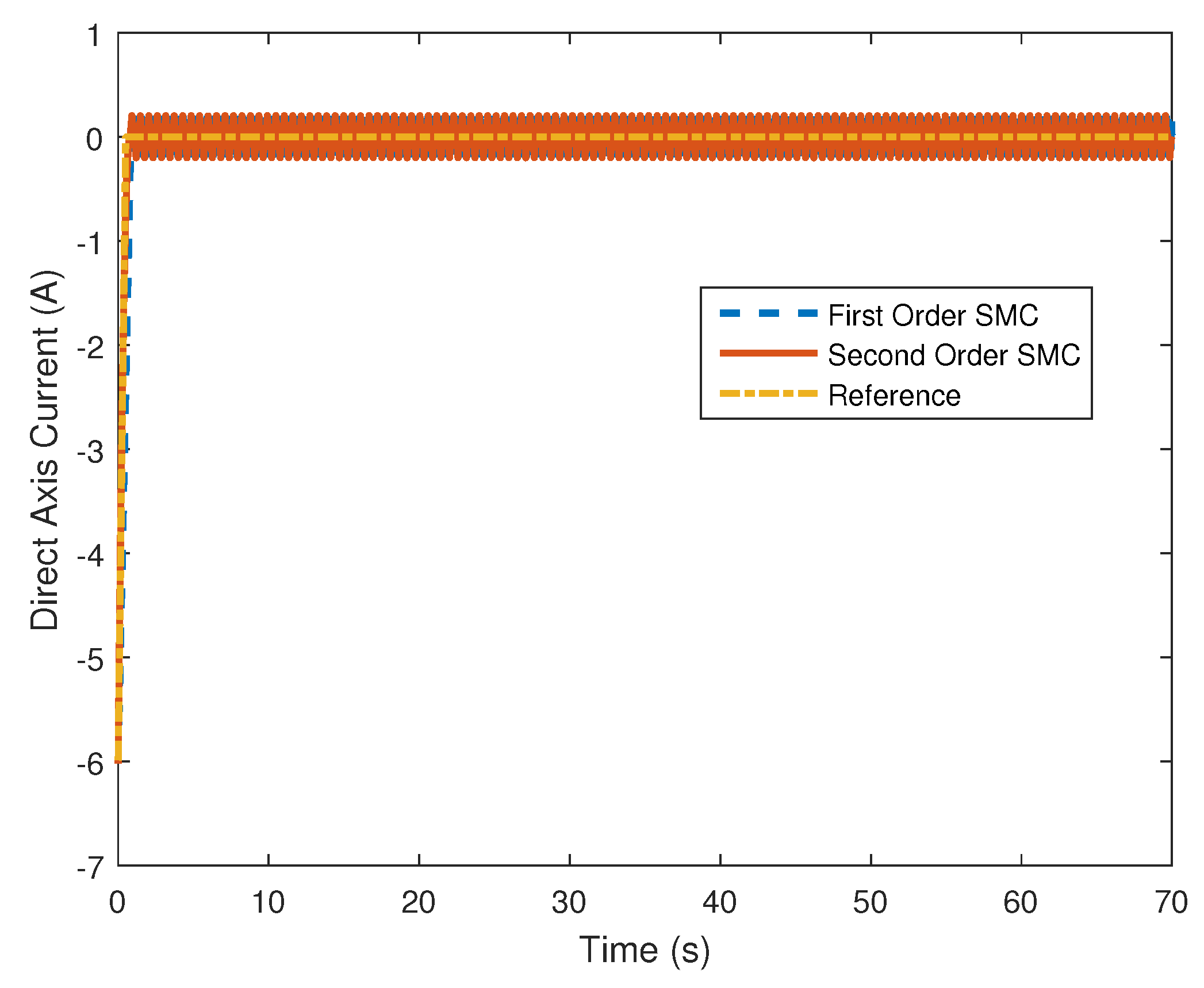
3.1.4. Direct Axis Current Control Design

In order to develop the d-axis control, Equation (29) must be satisfied. From Equation (22), this inequality can be re-written as:
s d ( t ) L - R s i d ( t ) + P 2 L i q ( t ) ω r ( t ) - u d ( t ) - L d i d ( t ) d t < 0
Denoting the d-axis control law as:
u d ( t ) = u d , e q ( t ) + u d , N ( t )
where u d , e q ( t ) is the equivalent control and u d , N ( t ) is the switching control. The equivalent control is given as follows:
u d , e q ( t ) = - R ^ s i d ( t ) + P 2 L ^ i q ( t ) ω r ( t ) - L ^ d i d ( t ) d t
Hence, s ˙ d from inequality Equation (32) becomes:
s ˙ d ( t ) = 1 Δ L - Δ R s i d ( t ) - Δ L d i d ( t ) d t - P 2 i q ( t ) ω r ( t ) - 1 Δ L u d , N ( t )
Due to the bounded nature of the uncertainties, along with the variables d i d ( t ) d t , i d ( t ) , i q ( t ) and ω r ( t ) , there exists a positive constant u d o , such that:
u d o > - Δ R s i d ( t ) + Δ L P 2 i q ( t ) ω r ( t ) - Δ L d i d ( t ) d t
From this, the switching portion of u d ( t ) is determined to be:
u d , N ( t ) = - u d o s g n ( s d ( t ) )
where:
s g n ( s ) = 1 , if   s > 0 0 , if   s = 0 - 1 , if   s < 0
The design of this controller should ensure that i d ( t ) is driven to i d ( t ) = 0 and will remain there despite disturbances.

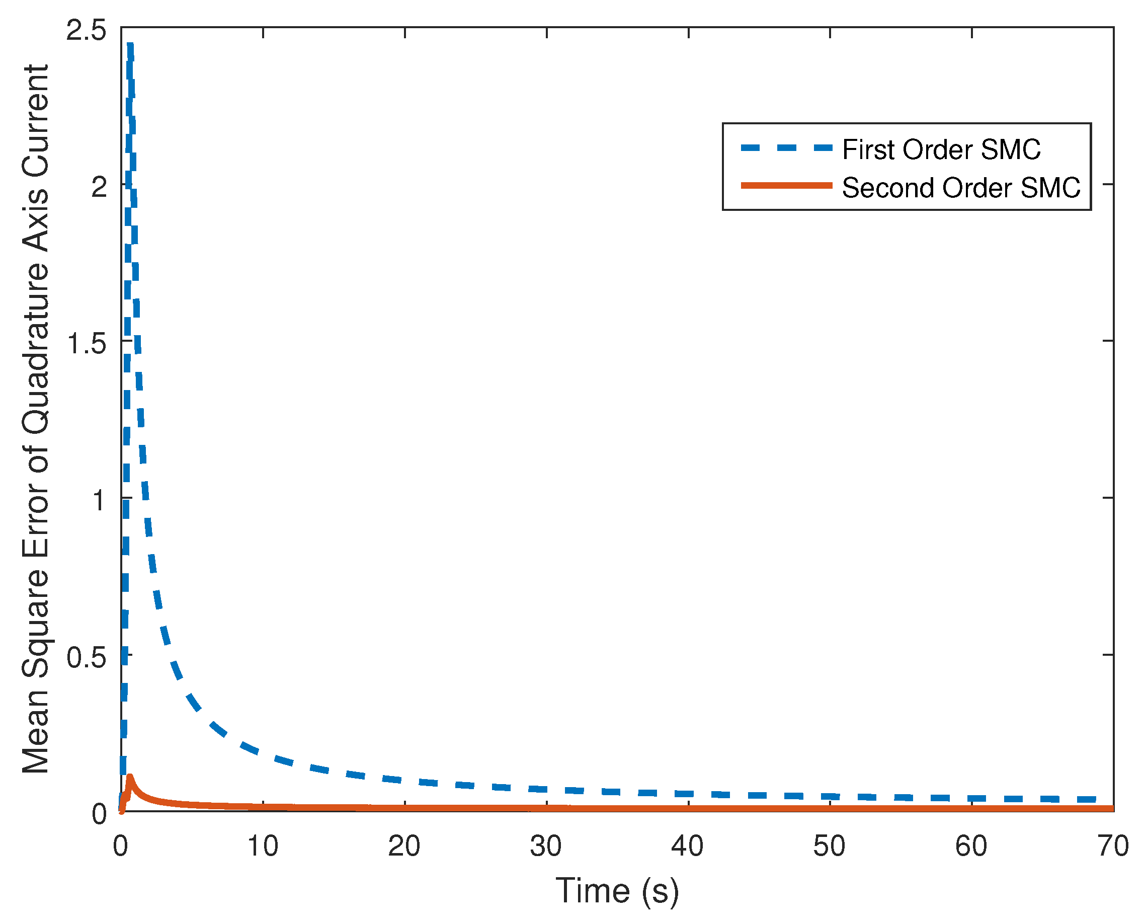
3.1.5. Quadrature Axis Control Design

Following the same method and considering the q-axis control, the inequality Equation (30) must be satisfied. Re-writing s ˙ q ( t ) in terms of Equations (23) and (26), Equation (30) can be re-written as:
s q ( t ) L - R s i q ( t ) - P 2 ( L i d ( t ) - Ψ m ) ω r ( t ) + s q ( t ) L - u q ( t ) - L d i q ( t ) d t < 0
Denoting the q-axis control law as the sum of the equivalent and switching controls respectively:
u q ( t ) = u q , e q ( t ) + u q , N ( t )
The equivalent control can be given as:
u q , e q ( t ) = - R ^ s i q ( t ) + P 2 ( L ^ i d ( t ) - Ψ ^ m ) ω r ( t ) - L ^ d i q ( t ) d t
Now, s ˙ q from inequality Equation (38) is written as:
s ˙ q ( t ) = 1 Δ L - Δ R s i q ( t ) - P 2 ( Δ L i d ( t ) - Δ Ψ m ) ω r ( t ) - 1 Δ L Δ L d i q ( t ) d t - u q , N ( t )
Again, due to the bounded nature of the uncertainties and variables, there exists a positive constant u q o , such that:
u q o > - Δ R s i q ( t ) - P 2 ( Δ L i q ( t ) + Δ Ψ m ) ω r ( t ) - Δ L d i d ( t ) d t
From this, the switching portion of u q ( t ) is determined to be:
u q , N ( t ) = - u q o s g n ( s q ( t ) )
The result of this control design should be that i q ( t ) is maintained at the reference i q ( t ) .

3.1.6. Control Design Based on Rotational Speed Dynamics

Again, making use of the similar method used for the d- and q-axis controls and ensuring that inequality Equation (31) is satisfied, s ˙ ω r ( t ) can be re-written from Equations (24) and (27). Equation (31) now becomes:
s ω r ( t ) K t τ m - K t i q ( t ) - B ω r ( t ) - J d ω r ( t ) d t < 0
For the rotational speed controller, the control variable becomes the quadrature axis reference current. It follows that the control law is designated:
i q ( t ) = i q , e q ( t ) + i q , N ( t )
With equivalent control:
i q , e q ( t ) = 1 K t τ ^ m - B ^ ω r ( t ) - J ^ d ω r ( t ) d t
s ˙ q from inequality Equation (44) is now re-written as:
s ˙ ω r ( t ) = 1 K t Δ τ m - Δ B ω r ( t ) - Δ J d ω r ( t ) d t
Based on previous reasoning for the d- and q-axis control design, there exists a positive constant i q o , such that:
i q o = 1 K t Δ τ m - Δ B - Δ J d ω r ( t ) d t
It then follows that:
i q , N ( t ) = - i q o s g n ( s ω r ( t ) )
This controller will actively control i q ( t ) . Therefore, the output is the input to the q-axis control developed previously.

3.2. Higher Order Sliding Mode Design Using Super Twisting Algorithm

To reduce the effect of chattering, higher order sliding mode control methods have been developed. The derivation of higher order sliding mode (HOSM) control is obtained using the super twisting algorithm. The sliding surfaces for HOSM control are chosen to be the same as the first-order type.

3.2.1. Direct Axis Control Design

For second-order sliding mode control, both s ( x ) and s ˙ ( x ) must be zero, so one more derivative of each function must be calculated. From the previous section, we have:
s ˙ d = 1 L [ - R s i d + P 2 ω r L i q - u d ] - d i d d t
from Equation (50), s ¨ d is found to be:
s ¨ d = - R s L d i d d t + P 2 d ω r d t i q + P 2 d i q d t ω r - 1 L d u d d t - d 2 i d d t 2
Denote:
ψ d = - R s L d i d d t + P 2 d ω r d t i q + P 2 d i q d t ω r - d 2 i d d t [ - Ψ d , Ψ d ]
and:
γ d = 1 L d u d d t [ Γ m , Γ M ]
The control input u d consists of the sum of two parts, u d , e q and u ˜ d , where u d , e q is the equivalent control (equal to the equivalent control found in the first-order sliding mode control), and u ˜ d is defined as:
u ˜ d = u d 1 + u d 2
where:
u ˙ d 1 = - W d s g n ( s d )
u d 2 = - λ | s 0 | p s g n ( s d ) | s d | > | s 0 | - λ | s d | p s g n ( s d ) | s d | | s 0 |
the corresponding sufficient conditions for finite time convergence to the sliding manifold are:
W d > Ψ d Γ m
λ 2 4 Ψ d Γ m 2 Γ M ( W d + Ψ d ) Γ m ( W d - Ψ d )
0 < p 0.5
The choice p = 0.5 ensures the maximum real sliding order two is achieved. Thus, we have:
u ˜ d = - λ | s d | 1 / 2 s g n ( s d ) - W d s g n ( s d ) d t
and the overall control is:
u d = u d , e q + u ˜ d

3.2.2. Quadrature Axis Control Design

The same method used for the direct axis is applied to the quadrature axis. Previously,
s ˙ q = 1 L [ - R s i q - P 2 ω r ( L i d - Φ m ) - u q ] - d i q d t
From Equation (62), we find s ¨ q to be:
s ¨ q = - R s L d i q d t - P 2 d i d d t ω r - P 2 ( i d - Φ m L ) d ω r d t - 1 L d u q d t - d 2 i q d t 2
Denote:
ψ q = - R s L d i q d t - P 2 d i d d t ω r - P 2 ( i d - Φ m L ) d ω r d t - d 2 i q d t 2 [ - Ψ q , Ψ q ]
and:
γ q = 1 L d u q d t [ Γ m , Γ M ]
u ˜ q = u q 1 + u q 2
where:
u ˙ q 1 = - W q s g n ( s q )
u q 2 = - λ | s 0 | p s g n ( s q ) | s q | > | s 0 | - λ | s q | p s g n ( s q ) | s q | | s 0 |
the corresponding sufficient conditions for finite time convergence to the sliding manifold are:
W q > Ψ q Γ m
λ 2 4 Ψ q Γ m 2 Γ M ( W q + Ψ q ) Γ m ( W q - Ψ q )
0 < p 0.5
Thus, we have:
u ˜ q = - λ | s q | 1 / 2 s g n ( s q ) - W q s g n ( s q ) d t
and the overall control is:
u q = u q , e q + u ˜ q

3.2.3. Quadrature Axis Current Reference Control Design

From the previous section,
s ˙ ω r = τ m J - K t J i q - B ω r J - d ω r d t
where K t = 3 P Φ m 4
From Equation (74), s ¨ ω r is:
s ¨ ω r = 1 J d τ m d t - K t J d i q d t - B J d ω r d t - d 2 ω r d t 2
Again, denote:
ψ ω = 1 J d τ m d t - B J d ω r d t - d 2 ω r d t 2 [ - Ψ ω , Ψ ω ]
and:
γ = - K t J d i q d t [ Γ m , Γ M ]
The overall control input is:
i q = i q , e q + i ˜ q
and:
i ˜ q = i q 1 + i q 2
where:
i ˙ q 1 = - W ω s g n ( s ω )
i q 2 = - λ | s 0 | p s g n ( s ω r ) | s ω r | > | s 0 | - λ | s ω r | p s g n ( s ω r ) | s ω r | | s 0 |
the corresponding sufficient conditions for finite time convergence to the sliding manifold are:
W ω r > Ψ ω r Γ m
λ 2 4 Ψ ω r Γ m 2 Γ M ( W ω r + Ψ ω r ) Γ m ( W ω r - Ψ ω r )
0 < p 0.5
Thus, we have:
i ˜ q = - λ | s ω r | 1 / 2 s g n ( s ω r ) - W ω r s g n ( s ω r ) d t
and the overall control is:
i q = i q , e q + i ˜ q

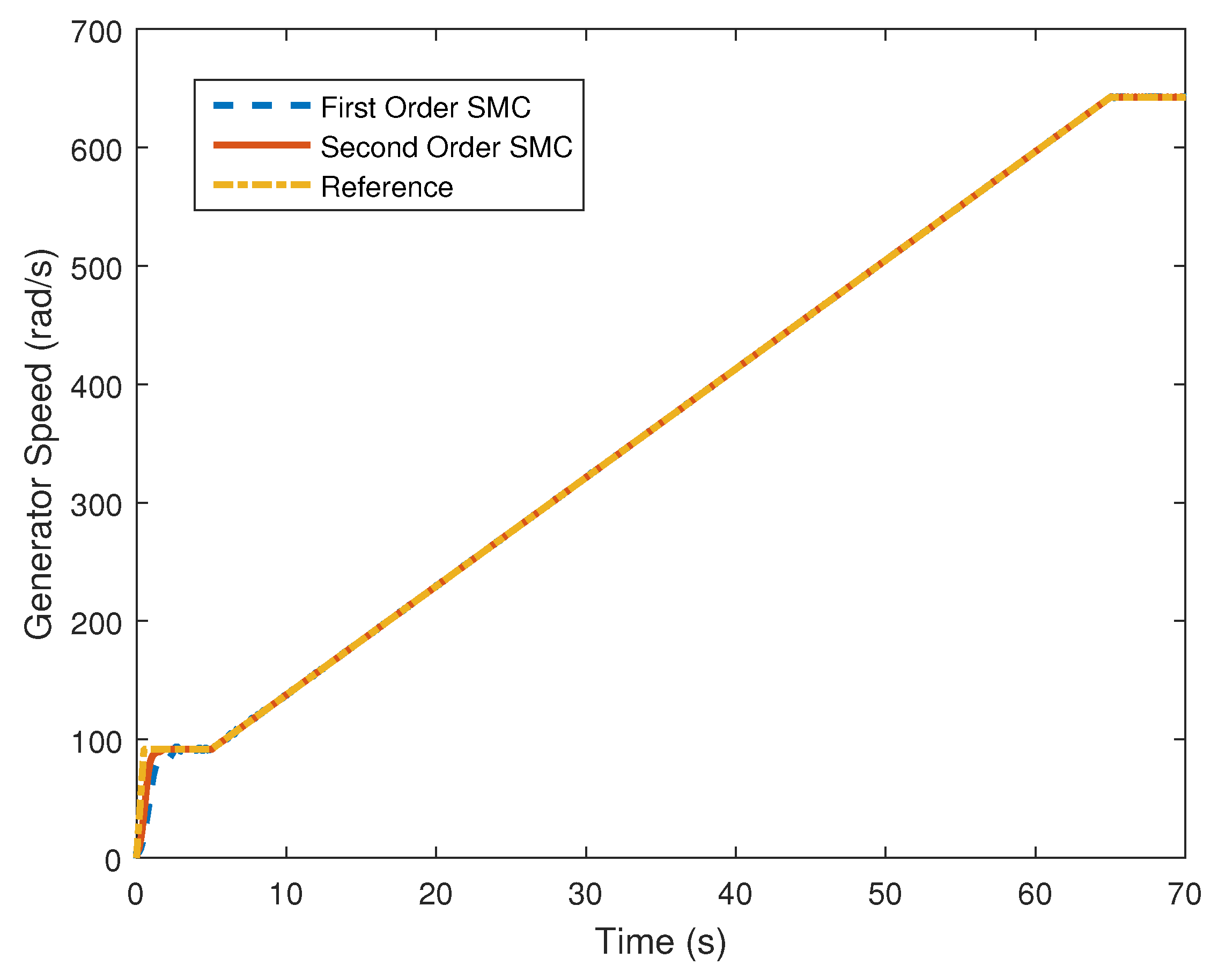
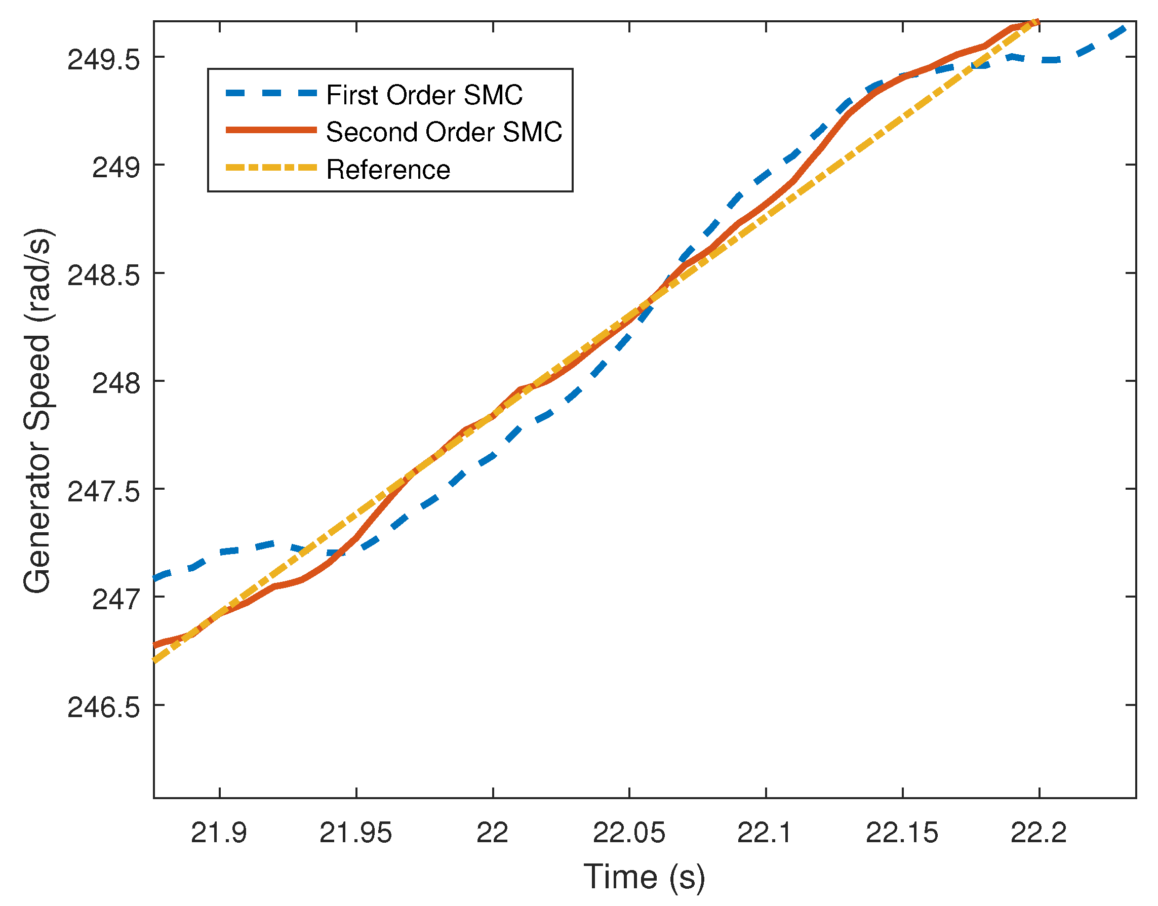
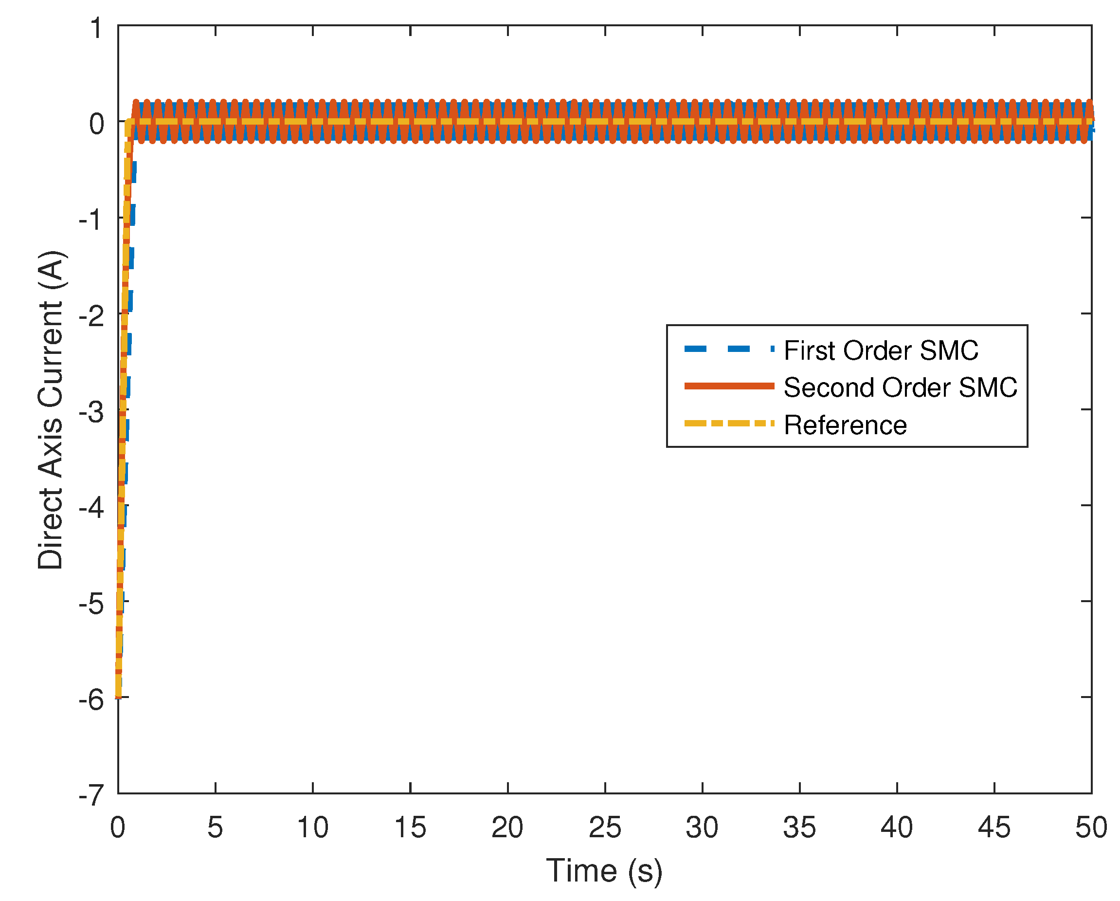
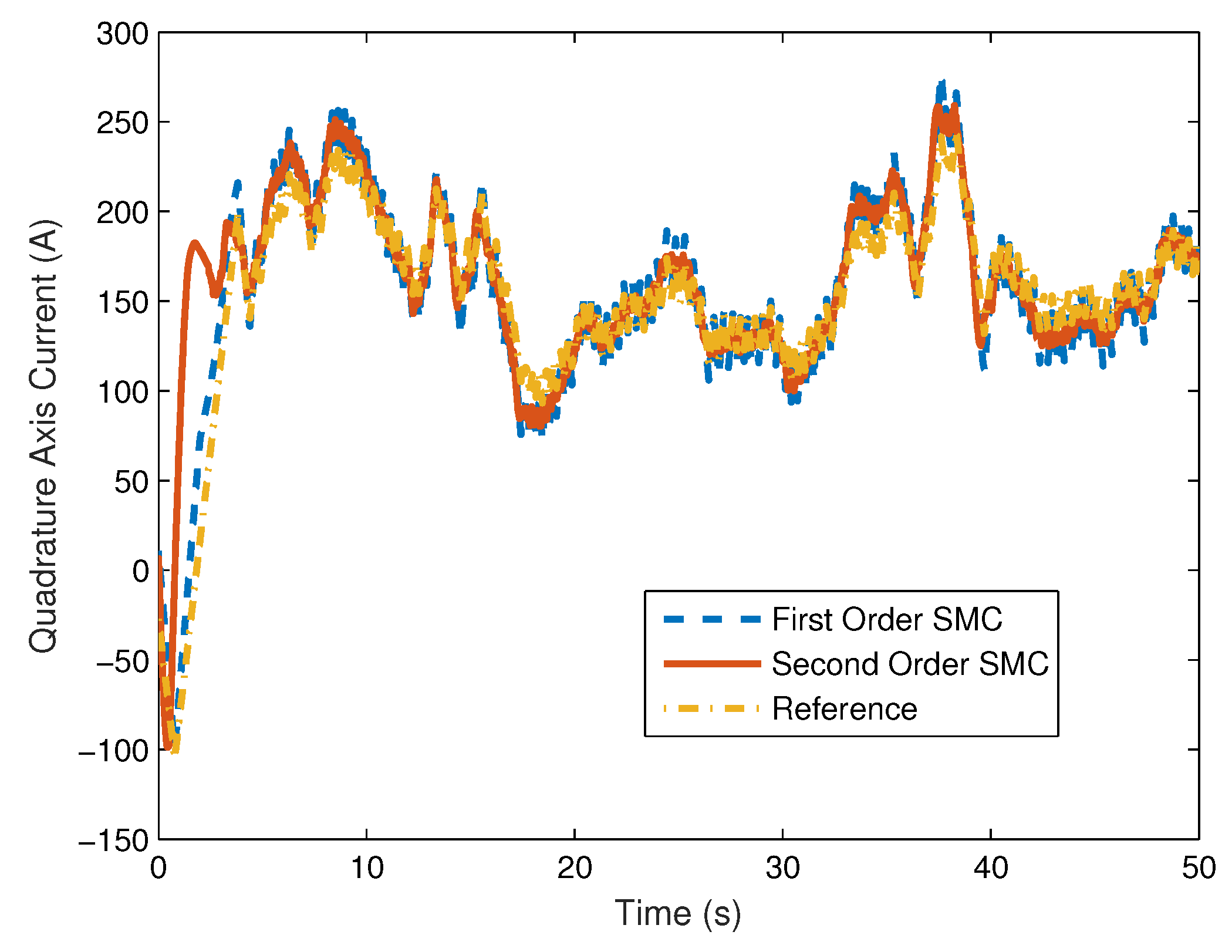
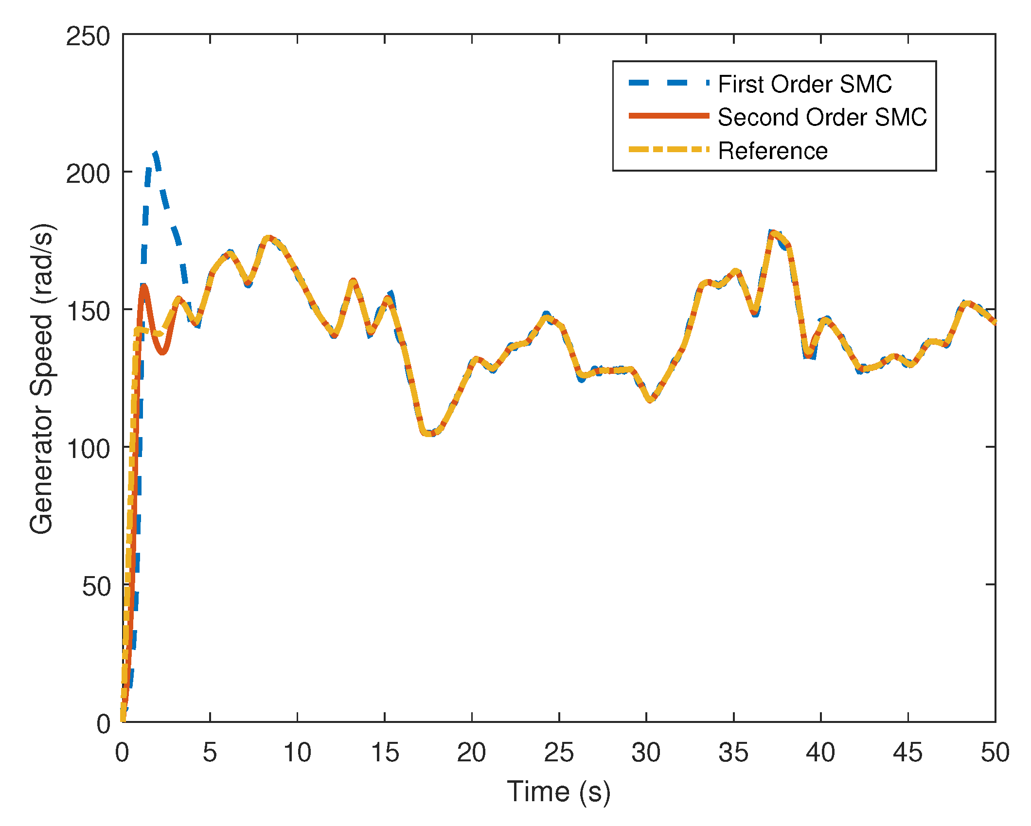
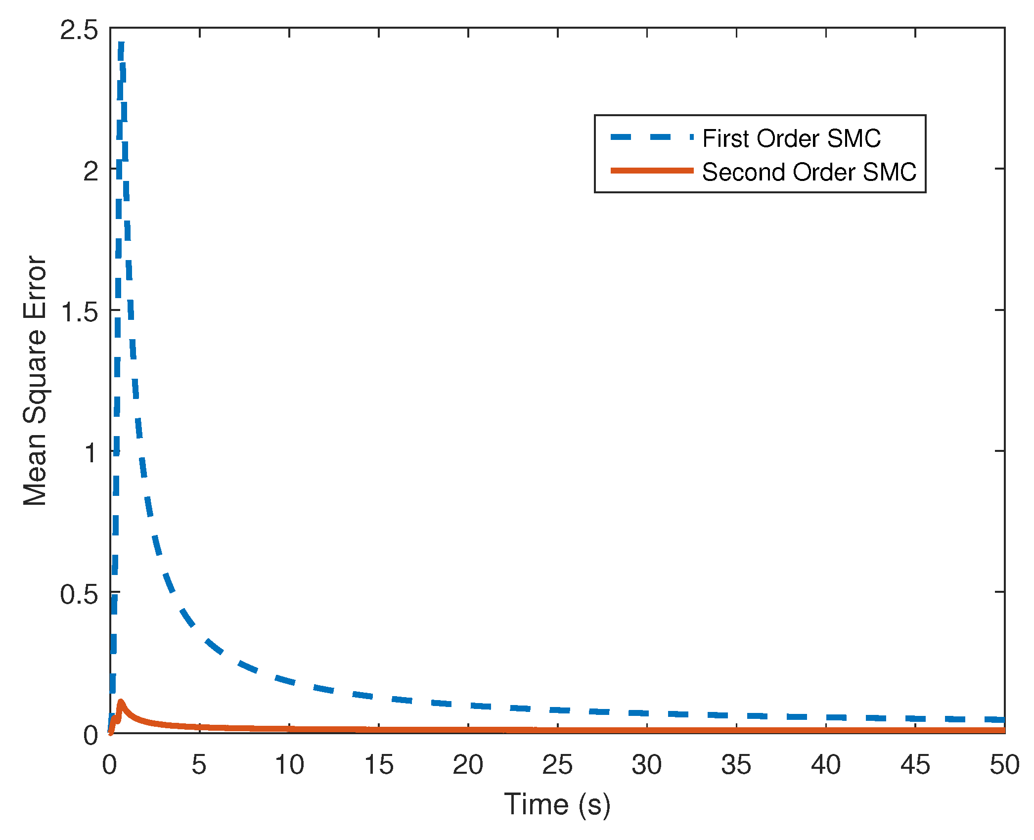
4. Computer Simulation Results

The implementation of the wind turbine aerodynamics, PMSG dynamics and SMC control architecture in MATLAB SIMULINK is shown by Figure 5. The nominal PMSG parameters used are listed in Table 1. Parameter variations were implemented within the Generator Dynamics block. The SIMULINK wind model in Figure 5 is capable of producing varying degrees of wind intensity and speed variations.
Two computer simulation studies are conducted with different wind speed profiles. In the first scenario, the wind speed input is piecewise affine. In the second scenario, the stochastic wind input is considered. Both simulation scenarios show the efficacy of the proposed approach.

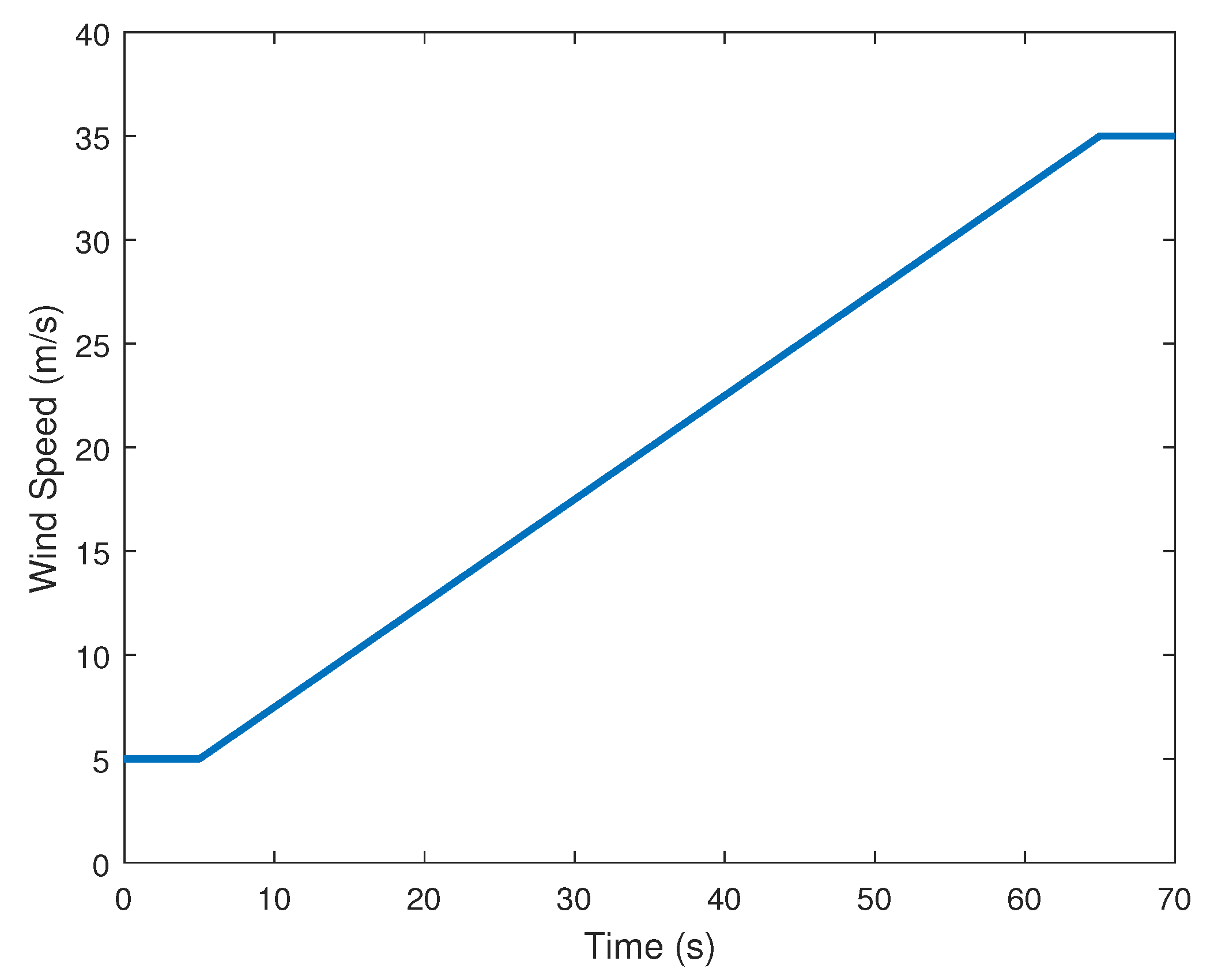
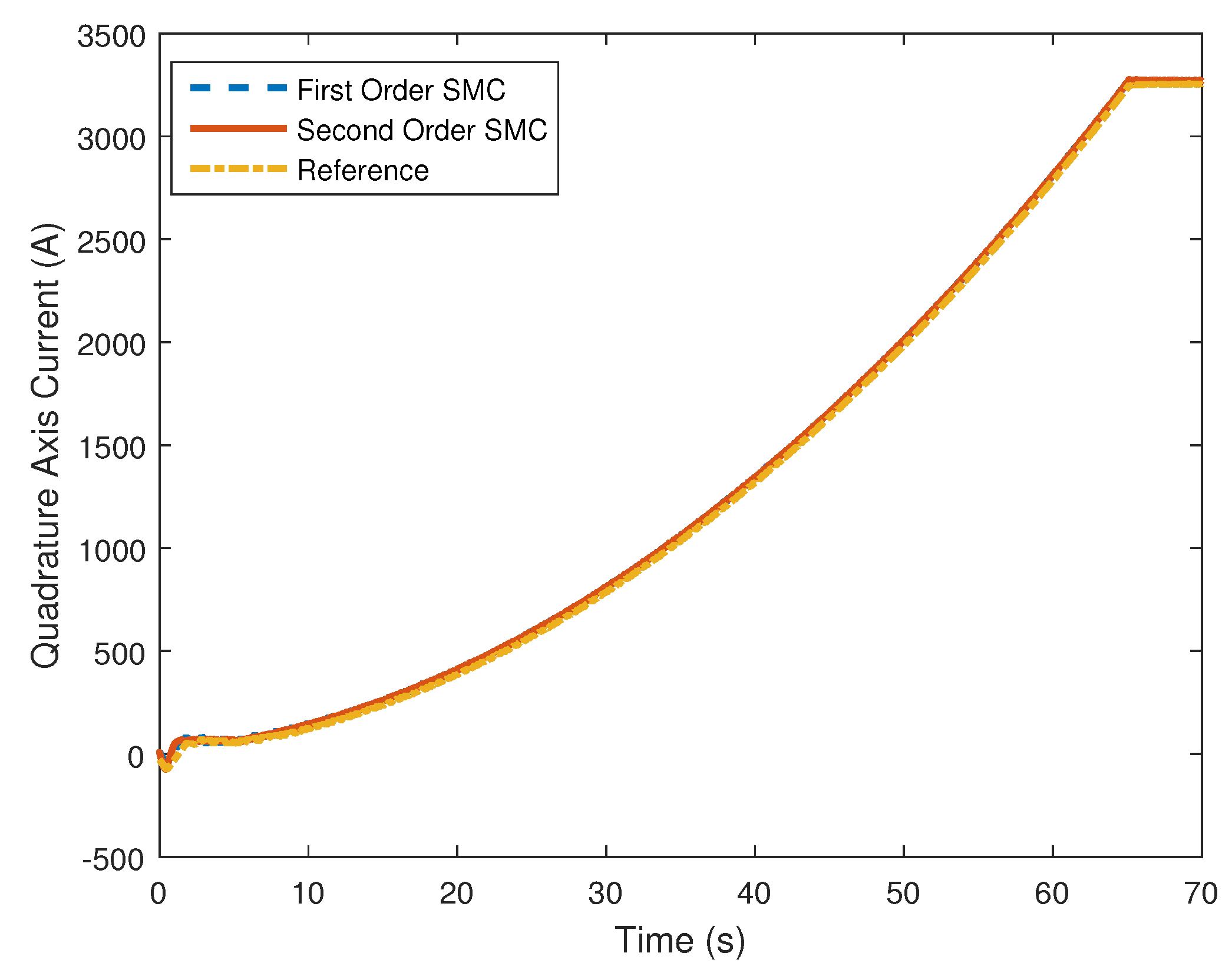
4.1. Piecewise Affine Wind Speed Input

Figure 6 shows the piecewise affine wind speed input, which is used to demonstrate the effectiveness of the proposed control approach. The range of varying speed is between 5 m/s and 35 m/s.
Both the stator direct axis current i d ( t ) and quadrature axis current i q are shown. As can be seen in Figure 7, the d-axis current accurately tracks the reference value i d ( t ) = 0 . Chattering about the reference with the first order sliding mode control is due to high frequency switching. However, despite constant fluctuations in wind speed, the d-axis control scheme effectively resists the effects of disturbances and parameter variations. The high order sliding mode control greatly improves the chattering effect. In Figure 8, the q-axis currents also accurately track the desired value i q ( t ) with both the first- and high order sliding mode controllers. Figure 9 shows the rotational speed ω r ( t ) accurately tracking the speed reference ω r ( t ) .
Inspection of these figures shows that accurate current and speed control are achieved, while the high order sliding mode control shows better accuracy and very significant chattering reduction. To better show the significant improvement of the high order SMC approach, the average mean square error (MSE) comparison of the i q state trajectory between the first and high order controllers is shown in Figure 10, where the exact effects of the chattering reduction can be seen. Figure 11 is a zoomed-in picture of Figure 9 between a short time period of 21.9 s and 22.2 s, which shows the better performance of the high order SMC in rotor speed ω r control.
The final and probably the most important result regards MPPT. Figure 12 shows the power coefficient corresponding to the piecewise affine wind profile in Figure 6. Immediately following the initial approach towards C p , m a x , it can be seen that the value of C p is held at or near C p , m a x despite all variations in the wind and system modeling uncertainties.

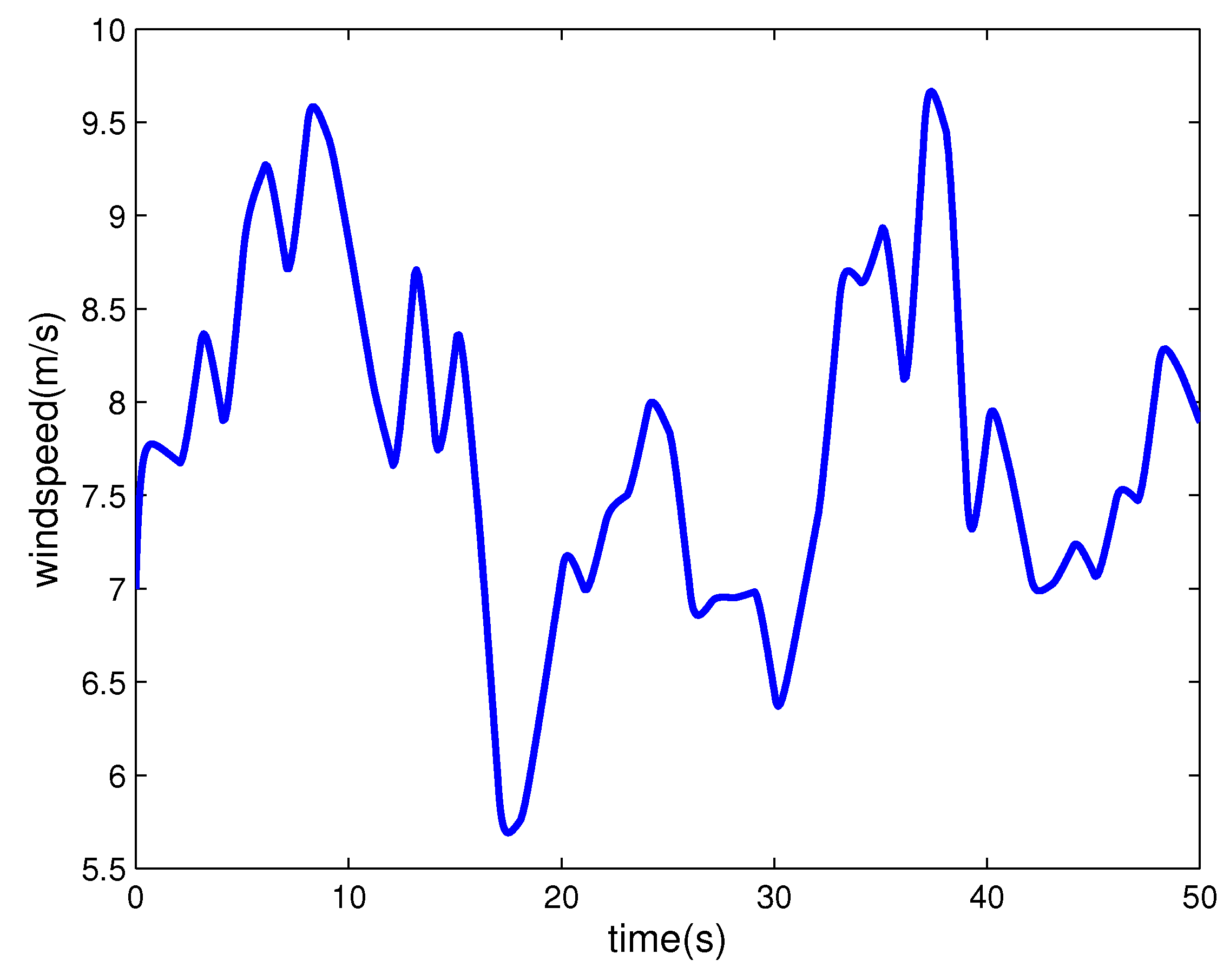
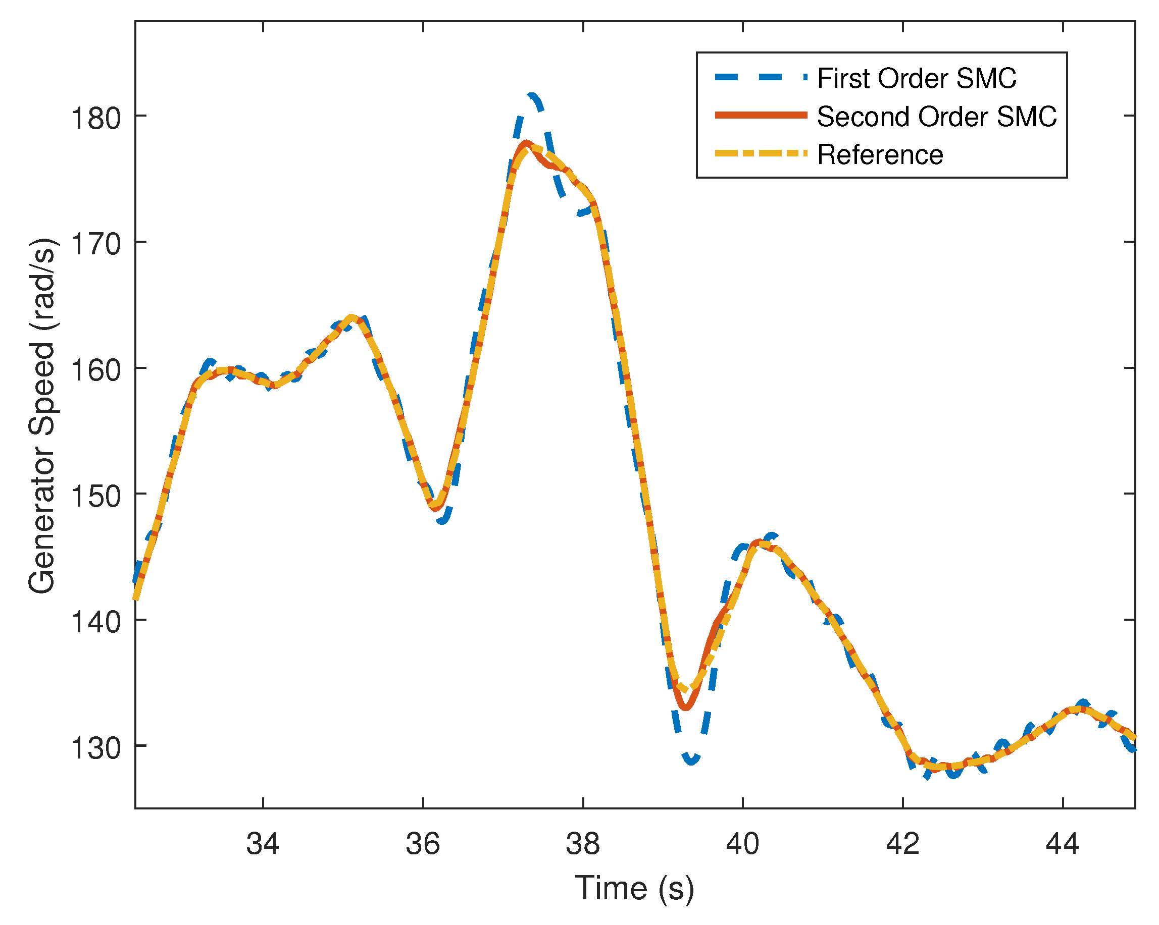
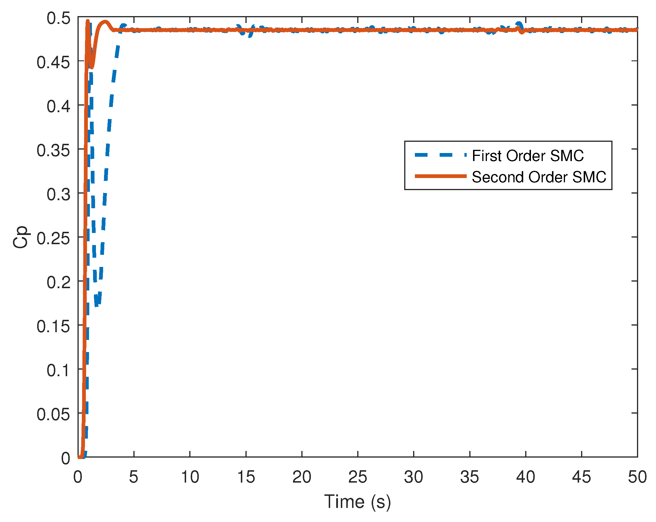
4.2. Stochastic Wind Speed Input

Figure 13 shows the stochastic wind input used for the remainder of the simulation results listed. For the second scenario, the stochastic wind input was chosen to demonstrate the effectiveness of the control design due to its highly varying nonlinear nature and the range of wind speeds.
The first result shown is that of i d ( t ) . As can be seen by Figure 14, the d-axis current accurately tracks the reference value i d ( t ) = 0 . Chattering about the reference with the first-order sliding mode control is due to switching delays. However, despite constant fluctuations in wind speed, the d-axis control scheme effectively resists the effects of disturbances and parameter variations. The high order sliding mode control significantly improves the chattering phenomenon.
One of the key components of the proposed control scheme is the active control of the quadrature axis current reference i q ( t ) through the implementation of a sliding mode controller based on the rotational speed dynamics of the WECS. Figure 15 shows the actual value of i q ( t ) , accurately tracking the defined reference i q ( t ) . Figure 16 shows the the rotational speed ω r ( t ) accurately tracking the speed reference ω r ( t ) . Inspection of these figures shows that accurate current and speed control are achieved, while the high order sliding mode control shows better accuracy and very significant chattering reduction. To better show the significant improvement of the high order SMC approach, the average MSE comparison of the i d state trajectory between the first- and high order controllers is shown in Figure 17, where the exact effects of the chattering reduction can be seen. Figure 18 presents a zoomed in section of Figure 16 to show the reduced chattering of the high order SMC in ω r after 38 s.
The final and probably the most important result regards MPPT. Figure 19 shows the power coefficient throughout the course of the simulation. Immediately following the initial approach towards C p , m a x , it can be seen that the value of C p is held at or near C p , m a x despite all fluctuations in the wind and parameters.
The proposed control algorithm will be realized in hardware for controlling the PMSG-based wind energy system in real time using the dSPACE DS1103 PPC system in future research studies.

5. Conclusions

The proposed first- and high order sliding mode controllers designed for a variable-speed surface-mounted PMSG-based WECS have been designed and simulated using MATLAB/SIMULINK. Preliminary testing of the novel control design results in a system with low sensitivity to disturbances and the ability to maintain a relatively constant level of power extraction efficiency in the presence of a highly varying wind input and bounded model parameter variations. Initial research into this method shows promise for active control of the quadrature axis current reference based on the use of an SMC control design for the dynamics of the high speed shaft rotational speed of the system. Testing with high order sliding mode controls shows vastly reduced chattering compared to a first-order sliding mode controller applied to the same model, even in highly variable wind conditions. This improved performance allows the WECS to maintain optimal power extraction efficiency without the side effects of chattering. Computer simulation results support this conclusion. However, the effectiveness of the proposed control topologies shows that they merit future research.

Acknowledgments

This is research work was funded by Southern Illinois University Edwardsville, Edwardsville, IL, USA.

Author Contributions

Guangping Zhuo, Jacob Hostettler, Patrick Gu designed and developed the system, performed the computer simulations and wrote the initial draft of the paper. Xin Wang supervised the project, provided technical guidance and insights, and carried out the final version of the paper.

Conflicts of Interest

The authors declare no conflict of interest.

References

  1. Singh, M.; Santoso, S. Dynamic Models for Wind Turbines and Wind Power Plants; Subcontract Report; National Renewable Energy Laboratory: Golden, CO, USA, October 2011.
  2. Orlando, N.A.; Liserre, M.; Mastromauro, R.A.; Dell’Aquila, A. A Survey of Control Issues in PMSG-Based Small Wind-Turbine Systems. IEEE Trans. Ind. Inform. 2013, 9, 1211–1221. [Google Scholar] [CrossRef]
  3. Errami, Y.; Ouassaid, M.; Maaroufi, M. Control of a PMSG based Wind Energy Generation System for Power Maximization and Grid Fault Conditions. Energy Procedia 2013, 42, 220–229. [Google Scholar] [CrossRef]
  4. Soraino, L.A.; Yu, W.; de Jesus Rubio, J. Modeling and Control of Wind Turbine. Math. Probl. Eng. 2013, 2013. [Google Scholar] [CrossRef]
  5. Munteanu, I.; Bratcu, A.I.; Cutulis, N.A.; Ceanga, E. Optimal Control of Wind Energy Systems; Springer: London, UK, 2008. [Google Scholar]
  6. Beltran, B.; El Hachemi Benbouzid, M.; Ahmed-Ali, T. Second-Order Sliding Mode Control of a Doubly Fed Induction Generator Driven Wind Turbine. IEEE Trans. Energy Convers. 2012, 27, 261–269. [Google Scholar] [CrossRef] [Green Version]
  7. Sharma, S.; Singh, B. Control of permanent magnet synchronous generator-based stand-alone wind energy conversion system. IET Power Electron. 2012, 5, 1519–1526. [Google Scholar] [CrossRef]
  8. Qiao, W.; Qu, L.; Harley, R.G. Control of IPM Synchronous Generator for Maximum Wind Power Generation Considering Magnetic Saturation. IEEE Trans. Ind. Appl. 2009, 45, 1095–1105. [Google Scholar] [CrossRef]
  9. Chinchilla, M.; Arnaltes, S.; Burgos, J.C. Control of permanent-magnet generators applied to variable-speed wind-energy systems connected to the grid. IEEE Trans. Energy Convers. 2006, 21, 130–135. [Google Scholar] [CrossRef]
  10. Beltran, B.; Ahmed-Ali, T.; Benbouzid, M. High-Order Sliding-Mode Control of Variable-Speed Wind Turbines. IEEE Trans. Ind. Electron. 2009, 56, 3314–3321. [Google Scholar] [CrossRef] [Green Version]
  11. Amimeur, H.; Aouzellag, D.; Abdessemed, R.; Ghedamsi, K. Sliding mode control of a dual-stator induction generator for wind energy conversion systems. Int. J. Electr. Power Energy Syst. 2012, 42, 60–70. [Google Scholar] [CrossRef]
  12. Munteanu, I.; Baccha, S.; Bractu, A.; Guiraud, J.; Roye, D. Energy-Reliability Optimization of Wind Energy Conversion Systems by Sliding Mode Control. IEEE Trans. Energy Convers. 2008, 23, 975–985. [Google Scholar] [CrossRef]
  13. Rajendran, E.; Kumar, C.; Rajesh-Kanna, R. Sliding Mode Controller based Permanent Magnet Synchronous Generator with Z-Source Inverter for Variable Speed Wind Energy Translation Structure using Power Quality Enhancement. Int. J. Comput. Appl. 2013, 75, 6–11. [Google Scholar] [CrossRef]
  14. Valenciaga, F.; Puleston, P.; Battaioto, P. Power Control of a Solar/Wind Generation System Without Wind Measurement: A Passivity/Sliding Mode Approach. IEEE Trans. Energy Convers. 2003, 18, 501–507. [Google Scholar] [CrossRef]
  15. Young, K.; Utkin, V.; Ozguner, U. A Control Engineer’s Guide to Sliding Mode Control. IEEE Trans. Control Syst. Technol. 1999, 7, 328–342. [Google Scholar] [CrossRef]
  16. Shtessel, Y.; Edwards, C.; Fridman, L.; Levant, A. Sliding Mode Control and Observation; Springer: New York, NY, USA, 2014. [Google Scholar]
  17. Levant, A. High-order sliding modes, differentiation, and output feedback control. Int. J. Control 2003, 76, 924–941. [Google Scholar] [CrossRef]
  18. Levant, A. Sliding order and sliding accuracy in sliding mode control. Int. J. Control 1993, 58, 1247–1263. [Google Scholar] [CrossRef]
  19. Bartolini, G.; Ferrara, A.; Usai, E. Chattering Avoidance by Second-Order Sliding Mode Control. IEEE Trans. Autom. Control 1998, 43, 241–246. [Google Scholar] [CrossRef]
  20. Bartolini, G.; Pisano, A.; Punta, E. A Survey of Applications of Second-order Sliding Mode Control to Mechanical Systems. Int. J. Control 2003, 76, 875–892. [Google Scholar] [CrossRef]
  21. Fridman, L.; Levant, A. Higher Order Sliding Mode Controls. In Sliding Mode Control in Engineering; CRC Press: New York, NY, USA, 2002. [Google Scholar]
  22. Phan, D.; Huang, S. Super-Twisting Sliding Mode Control Design for Cascaded Control System of PMSG Wind Turbine. J. Power Electron. 2015, 15, 1358–1366. [Google Scholar] [CrossRef]
  23. Laghrouche, S.; Plestan, F.; Glumineau, A.; Boisliveau, R. Robust second order sliding mode control for a permanent magnet synchronous motor. In Proceedings of the 2003 American Control Conference, Denver, CO, USA, 4–6 June 2003; pp. 4071–4076.
  24. Laghrouche, S.; Plestan, F.; Glumineau, A. Higher order sliding mode control based on optimal linear quadratic control. In Proceedings of the 2003 European Control Conference (ECC), Cambridge, UK, 1–4 September 2003.
  25. Beltran, B.; Benbouzid, T.; Ahmed-Ali, T. High-Order Sliding Mode Control of a DFIG-Based Wind Turbine for Power Maximization and Grid Fault Tolerance. In Proceedings of the 2009 IEEE International Electric Machines and Drives Conference, Miami, FL, USA, 3–6 May 2009.
  26. Valenciaga, F.; Puleston, P. High-Order Sliding Control for a Wind Energy Conversion System Based on a Permanent Magnet Synchronous Generator. IEEE Trans. Energy Convers. 2008, 23, 860–867. [Google Scholar] [CrossRef]
  27. Plestan, F.; Glumineau, A.; Laghrouche, S. A New Algorithm for High-Order Sliding Mode Control. Int. J. Robust Nonlinear Control 2007, 18, 441–453. [Google Scholar] [CrossRef]
  28. Wang, X.; Alden, M.J. Resilient and Robust Control of Time-Delay Wind Energy Conversion Systems. ASME J. Risk Uncertainty Part B 2016, 3, 1–8. [Google Scholar] [CrossRef]
  29. Betz, A. Introduction to the Theory of Flow Mechanics; Pergamon Press: Oxford, UK, 1966. [Google Scholar]
  30. Garcia-Sans, M.; Houpis, C. Wind Energy Systems Control Design; Taylor & Francis Group, LLC: Boca Raton, FL, USA, 2012. [Google Scholar]
  31. Munteanu, I.; Bratcu, A.; Cutululis, N.; Ceanga, E. Optimal Control of Wind Energy Systems Towards a Global Approach; Springer: London, UK, 2008. [Google Scholar]
  32. Molina, M.; Alvarez, J. Wind Farm—Technical Regulations, Potential Estimation and Siting Assessment; InTech: Rijeka, Croatia, 2011. [Google Scholar]
Figure 1. Model of actuator disk interaction with wind [28].
Sustainability 08 01265 g001
Figure 2. Simplified diagram of a permanent magnet synchronous generator (PMSG)-WECS [28].
Sustainability 08 01265 g002
Figure 3. C p power coefficient vs. tip speed vs. pitch angle.
Sustainability 08 01265 g003
Figure 4. C q torque coefficient vs. tip speed vs. pitch angle.
Sustainability 08 01265 g004
Figure 5. Overall MATLAB simulation model.
Sustainability 08 01265 g005
Figure 6. Piecewise affine wind speed input.
Sustainability 08 01265 g006
Figure 7. The direct axis current i d state trajectory controlled by the sliding mode control (SMC).
Sustainability 08 01265 g007
Figure 8. The quadrature axis current i q state trajectory controlled by the SMC.
Sustainability 08 01265 g008
Figure 9. The rotational speed ω r state trajectory controlled by the SMC.
Sustainability 08 01265 g009
Figure 10. MSE comparison of i q state trajectory with first- and high order SMC.
Sustainability 08 01265 g010
Figure 11. The “zoomed in” ω r state trajectory to show the chattering effect.
Sustainability 08 01265 g011
Figure 12. Power coefficient.
Sustainability 08 01265 g012
Figure 13. Stochastic wind input.
Sustainability 08 01265 g013
Figure 14. The direct axis current i d state trajectory controlled by the SMC.
Sustainability 08 01265 g014
Figure 15. The quadrature axis current i q state trajectory controlled by the SMC.
Sustainability 08 01265 g015
Figure 16. The rotational speed ω r state trajectory controlled by the SMC.
Sustainability 08 01265 g016
Figure 17. MSE comparison of i d state trajectory with first- and high order SMC.
Sustainability 08 01265 g017
Figure 18. The “zoomed in” ω r state trajectory to show the chattering effect.
Sustainability 08 01265 g018
Figure 19. Power coefficient.
Sustainability 08 01265 g019
Table 1. Turbine and generator parameters.
PropertyParameter Value
Rotor radius R t = 3 m
Stator Resistance R s = 3.5 Ω
d-axis inductance L q = 35 mH
q-axis inductance L d = 35 mH
Flux linkage Ψ m = 0.3 Wb
Poles P = 6
Inertia J = 1
Stiffness B = 0.001

