Impact of Battery’s Model Accuracy on Size Optimization Process of a Standalone Photovoltaic System

Abstract

This paper presents a comparative study between two proposed size optimization methods based on two battery’s models. Simple and complex battery models are utilized to optimally size a standalone photovoltaic system. Hourly meteorological data are used in this research for a specific site. Results show that by using the complex model of the battery, the cost of the system is reduced by 31%. In addition, by using the complex battery model, the sizes of the PV array and the battery are reduced by 5.6% and 30%, respectively, as compared to the case which is based on the simple battery model. This shows the importance of utilizing accurate battery models in sizing standalone photovoltaic systems.

1. Introduction

The atmospheric carbon dioxide (CO2) emission problems and the rapid depletion of fossil fuel sources worldwide encourage researchers to search for alternative sources that are clean and environment friendly. Photovoltaics (PV) have attracted the energy sector to be considered as power generating sources as they are clean and secure [1]. Standalone PV systems are becoming increasingly viable and cost-effective for supplying electricity to rural areas. However, the drawback of standalone PV systems is the high capital cost as compared with conventional energy sources. To reduce the capital cost, an optimal sizing process of a standalone PV system is necessary so as to achieve a relatively reliable system at minimum cost [2]. Standalone PV system size depends on meteorological variables, such as solar radiation and ambient temperature. This is due to the fact that the performance of a standalone PV system strongly depends on the availability of solar radiation and the ambient temperature [3]. In addition to that, the utilized system’s models also strongly affects the sizing results as it reflects the performance of the system.

Currently, many size optimization methods are proposed in order to select the optimal number of PV modules and the capacity of the storage battery. A study was done for optimal sizing of a standalone PV system in Kuala Lumpur, Malaysia by Shen [4] considering a fixed tilt angle and continuous solar radiation variation. The methodology starts by calculating the daily output energy of a solar array as a function of peak sunshine hours, ambient temperature, and accumulative dust losses. Then, the PV array daily energy output, the inverter efficiency, the load demand, the battery storage energy, and the battery charge/discharge efficiencies are used to estimate the daily state of charge (SOC) of the battery. The loss of power supply probability (LPSP) is defined and the system’s cost is formulated in a way that includes the costs of the battery, the PV array, and other components. The equation of the system’s cost is partially derived and solved graphically. As a result, two curves are drawn which represent the different size combinations of the PV array and the storage battery for the desired LPSP. The tangent point of the presented curves indicates the optimum size of the PV/battery combination. This method has a limitation in which sizing curves have to be constructed for each particular load demand.

Meanwhile, an analytical method was developed by Khatib et al. [5] for optimal sizing of a PV/battery configuration of a standalone PV system in Malaysia. The developed method was carried out by deriving size formulas for the size of PV array and battery which can be generalized for Malaysia and nearby zones. Firstly, the sizing methodology defines some constants, such as the specifications of the system and the load demand. Here, daily average meteorological and load demand data are used for this purpose. Then, the size of the PV array and the capacity of the storage battery are calculated based on a specific loss of load probability (LLP). The authors plot the LLP values versus the PV array size and PV array size versus the battery capacity. Then MATLAB fitting toolbox is used to estimate the coefficients of these formulas. This research work has some limitations in which a simple battery model is used, daily average meteorological data are utilized, and the method is not taking into consideration any economical parameters. In conclusion, these limitations may affect the accuracy of the sizing results.

In 2016, Nordin and Rahman [6] proposed a novel optimization method for sizing a standalone PV system using numerical methods. The sizing methodology was done based on Malaysian’s weather profile. Hourly meteorological and load demand data were utilized to verify the novelty of the proposed method. The authors assumed a design space that specifies the numbers of the PV modules and storage battery unites. Then, the LPSP is obtained for each combination in the design space. As a result, all the combinations that have the desired LPSP are selected for the second stage which is the calculation of the levelized cost of energy (LCE). Following that, the optimum PV/battery combination is chosen based on the minimum value of the LCE. Here, a simple linear PV array model and a dynamic battery model have been used to model the performance of the system. Therefore, the numerical method is the most frequently used method for optimally sizing a standalone PV system. Numerical method is mainly done in terms of a bi-objective techno-economic optimization function which is formulated based on the best trade-off between system’s cost and availability [7]. Therefore, with the numerical method, four aspects must be considered to accurately size a standalone PV system, which are input data, system’s models, simulation methods, and formulated objective function [8].

In previous works, simple battery models have been used to represent the charging and discharging process in sizing algorithms of standalone PV systems [9,10]. Meanwhile, some more complex battery models are utilized [11,12]. Simple battery models can be defined as a series of mathematical equations that express the status of the storage of a battery without reflecting the dynamic behavior of the charging and discharging processes. Simple battery models may affect the accuracy of the sizing results as the state of charge of the battery is not calculated accurately. In contrast, complex battery models consider the dynamic behavior of the battery during charging and discharging process. Thus, the accuracy of the sizing results is expected to be higher.

Based on this, in this paper, a comparative study is done between two sizing algorithms that are based on simple and complex battery models. Experimental data of a 3 kWp PV system installed at the Universiti Kebangsaan Malaysia campus are used for this purpose. These data contain hourly solar radiation, ambient temperature, and actual system output.

2. Modeling of a Standalone PV system

In general, the typical standalone PV/battery power system is usually consisted of a PV array, storage device, and power electronics devices, such as DC/DC converter and DC/AC inverter. However, in modeling a standalone PV system as a power system, the most important models are the PV array and storage battery models, which reflect the power flow inside the performance of the system. As for the power electronic devices, such DC/DC converters and DC/AC inverters, the conversion efficiencies are usually assumed for in process.

2.1. Photovoltaic Panels

In [13], the PV array output is modeled in terms of energy using a linear model. According to these studies, the output of the PV array is given by:

$$E_{PV}=A_{PV}\times E_{sun}\times {\eta }_{PV}\left(t\right)\times {\eta }_{inv}\times {\eta }_{wire}$$

(1)

where $A_{PV}$ represents the area of the PV module ($m^2$), $E_{sun}$ is the hourly solar energy ($wh/m^2$), ${\eta }_{PV}$ represents the efficiency of the PV module, ${\eta }_{inv}$ is the efficiency of the inverter, and ${\eta }_{wire}$ is the efficiency of the wires.

In addition, the effect of temperature on the conversion efficiency of the PV model is obtained by:

$${\eta }_{PV}\left(t\right)={\eta }_{PV,ref}\left[1-\beta \left(T_C\left(t\right)-T_{C,ref}\right)\right]$$

(2)

where ${\eta }_{PV,ref}$ is the reference PV module efficiency, $\beta$ is temperature coefficient for the efficiency, $T_{C,ref}$ is reference cell temperature, and $T_C\left(t\right)$ is the cell temperature which can be calculated by:

$$T_C\left(t\right)=T_A\left(t\right)+\left(\frac{NOCT-20˚}{800}\right)\times G\left(t\right)$$

(3)

where $T_A$ is the ambient temperature, $G$ is the solar radiation, and $NOCT$ is the nominal operating cell temperature which is usually supplied by the manufacturer. $NOCT$ is defined as the operating temperature of a PV module under solar radiation ($G$) of 800 $w/m²$, ambient temperature ($T_A$) of 20 $˚C$, and wind speed ($v_w$) of 1 $m/sec.$

This model is clearly too simple. The shadowing phenomena and the parametric differences in the solar cells are not taking into account. Moreover, with this model, it is assumed that all the solar cells in the PV module are identical and received the same quantity of solar radiation and temperature conditions. However, this simplicity does not affect the aim of this research work. The aim is focused on studying the effects of the storage battery’s models on the sizing results.

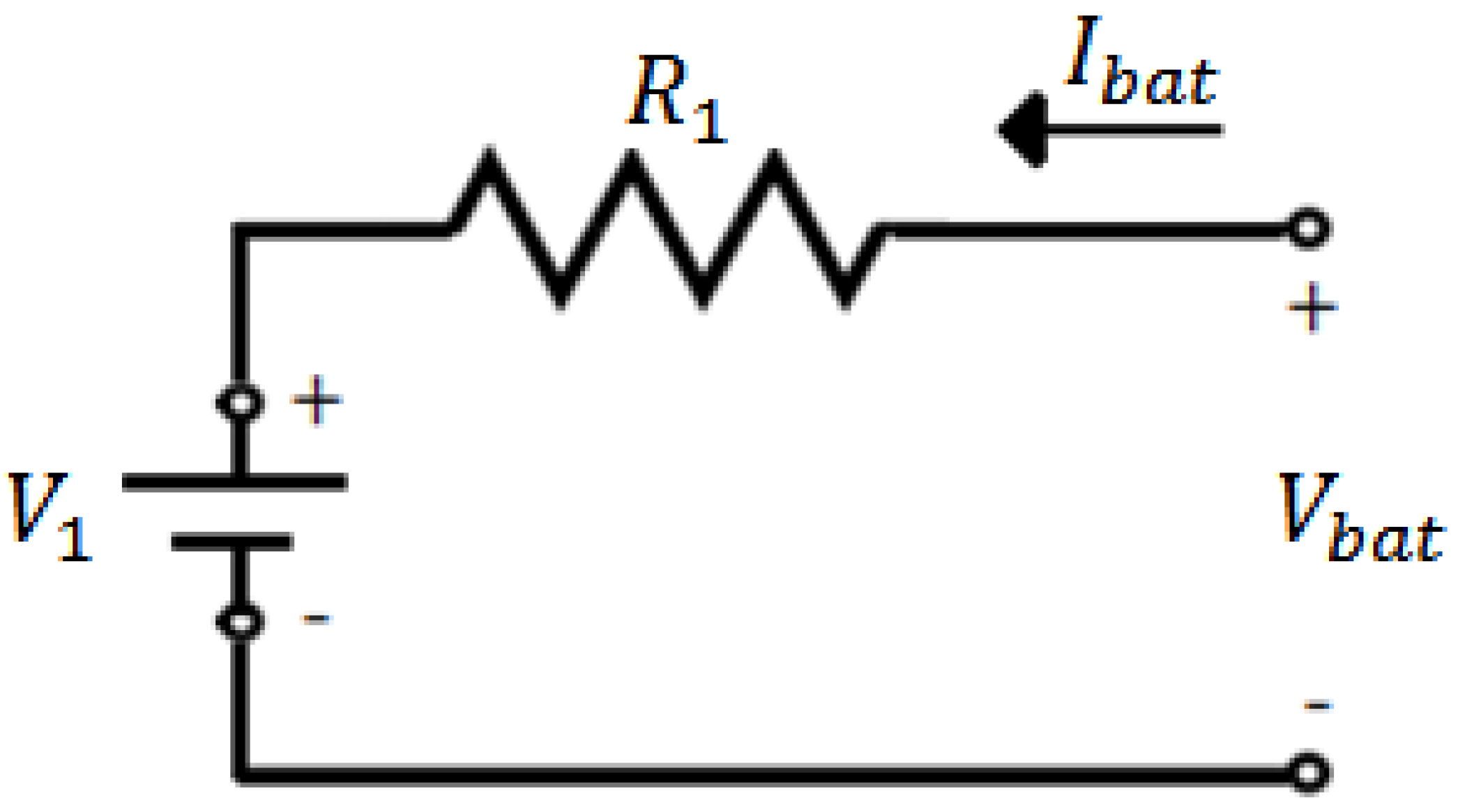
2.2. Utilized Battery Model

In [13], a static battery model is utilized in a standalone PV system size optimization. This model can be defined as a series of equations that express the status of the battery without reflecting the dynamic behavior of the battery’s charging and discharging processes. This model is mainly based on a predefined term namely the energy difference ($E_D\left(t\right)$) which is given by:

$$E_D\left(t\right)={\displaystyle \sum }_{t=1}^{8765}(E_{PV}\left(t\right)-E_L\left(t\right))$$

(4)

where $E_L\left(t\right)$ and $E_{PV}\left(t\right)$ are the instantaneous hourly load demand, energy produced by PV array, respectively.

If the result of $E_D\left(t\right)$ is positive ($E_{PV}\left(t\right)>E_L\left(t\right)$) then $E_D\left(t\right)$ shows an excess energy ($E_{excess}$). However, if the result of $E_D\left(t\right)$ is negative ($E_{PV}\left(t\right)<E_L\left(t\right)$) then $E_D\left(t\right)$ shows a deficit energy ($E_{deficit}$). Finally, if the result of $E_D\left(t\right)$ is zero ($E_{PV}\left(t\right)=E_L\left(t\right)$) then there is no excess or deficit energy ($E_{excess}$, and $E_{deficit}$ are equal zero).

Then, the instantaneous value of the state of charge of the battery model ($SO{C}_n\left(t\right)$) in [13] is calculated as:

$$SO{C}_n\left(t\right)=\{\begin{array}{c}SOCmax,SOCmax+E_D\left(t\right)>SOCmax\\ SOCmin,SOCmax+E_D\left(t\right)<SOCmin\\ SOCmax+E_D\left(t\right),other wise\end{array}$$

(5)

On the other hand, other authors utilized more complex models [14,15]. Figure 1 shows the equivalent electrical circuit of a lead-acid battery. The battery’s internal voltage is expressed as a voltage source ($V_1$), and internal resistance ($R_1$). The charging and discharging processes are mainly depending on the direction of the current of battery ($I_{bat}$) which depends on the voltage difference between the voltage of the battery ($V_{bat}$) and $V_1$ [1]:

The energy storage capacity of the battery can be calculated by the following relation [15]:

$$E_{bat}=d_0\left(\frac{E_{tot}}{8760}\right)\frac{1}{{\eta }_{batt}}.\frac{1}{DO{D}_L}=d_0.\frac{E_h}{{\eta }_{batt}}.\frac{1}{DO{D}_L}$$

(6)

where $d_0$ is the typical hours of energy autonomy, $E_{tot}$ is the annual energy of the load, ${\eta }_{batt}$ is the energy transformation efficiency, $DO{D}_L$ is the maximum depth of discharge, and $E_h$ is the average hourly energy of the load.

Moreover, the nominal input ($P_{bat\_in}$) and output power ($P_{bat\_out}$) can be obtained by:

$$P_{bat\_in}=\mathsf{{\rm Y}}.P_{bat\_out}\le P_{PV}$$

(7)

where $\mathsf{{\rm Y}}$ is represented the ratio of charge and discharge periods as well as the energy transformation efficiency in the battery. However, $\mathsf{{\rm Y}}$ is in the range of 1.5–3 [15]:

$$P_{bat\_out}=\zeta .\frac{E_h}{C{F}_{load}}.\frac{1}{{\eta }_p}$$

(8)

where $\zeta$ is the peak power percentage of the load the battery should cover, $C{F}_{load}$ is the capacity factor, and ${\eta }_p$ is the power efficiency.

The state of charge ($SOC$) of battery can be mathematically formulated as [16]:

$$SOC=1-\frac{Q}{C},0\le SOC\le 1$$

(9)

where $Q$ is the battery charge, and $C$ is the nominal battery capacity.

The depth of charge ($DOD$) of battery can be represented as:

$$DOD=1-SOC$$

(10)

From $DOD$ value, the minimum $SOC$ of the battery can be calculated by:

$$SOCmin=SOCmax\left(1-DOD\right)$$

(11)

where $SO{C}_{max}$ is the maximum $SOC$ of the battery.

The state of charge of the battery ($SOC$) can be calculated in charging and discharging mode as the following equation [16]:

$$SOC\left(1+dt\right)=SOC\left(t\right)\left[1-\frac{D}{3600}.dt\right]+K\left[\frac{V_{bat}{I}_{bat}-R_x{I}_{bat}²}{3600}\right].dt$$

(12)

where $D$ is the charging efficiency rate, $K$ is the self-efficiency rate, $V_{bat}$ is the battery voltage, which depends on the battery mode, $I_{bat}$ is the battery current, and $R_x$ is the charging resistance ($R_{ch}$) or discharging resistance ($R_{dch}$) which depends on the battery mode.

Meanwhile, the instantaneous value of state of charge of the battery model ($SO{C}_n\left(t\right)$) can be estimated as:

$$SO{C}_n\left(t\right)=SO{C}_0+\frac{1}{SO{C}_{max}}+\int [\frac{K{V}_{bat}{I}_{bat}}{3600}-\frac{D.SO{C}_n\left(t-\tau \right)SO{C}_{max}}{3600}]dt$$

(13)

where $SO{C}_0$ is the initial $SOC$ of the battery, $SO{C}_{max}$ is the maximum $SOC$ of the battery, and $\tau$ is the internal time step of the simulation.

In charge mode, the battery voltage ($V_{bat}$) can be obtained as the following equation [16]:

$$V_{bat}=V_{ch}+I_{bat}{R}_{ch}$$

(14)

where $V_{ch}$ is the charging voltage which can calculated by,

$$V_{ch}=\left(2+0.148\beta \right)N_s$$

(15)

The charging resistance ($R_{ch}$) can be obtained by:

$$R_{ch}=\left[\frac{0.758+\frac{0.1309}{1.06+\beta }}{SO{C}_{max}}\right]N_s$$

(16)

where $N_s$ is the number of 2 V series cells in the battery, and $\beta$ is expressed the ratio of the initial $SOC$ of the battery ($SO{C}_0$) to maximum $SOC$ of the battery ($SO{C}_{max}$), which is mathematically represented as:

$$\beta =\frac{SO{C}_0}{SO{C}_{max}}$$

(17)

On the other hand, the battery voltage ($V_{bat}$) can be formulated in the discharge mode as the following equation [16]:

$$V_{bat}=V_{dch}+I_{bat}{R}_{dch}$$

(18)

where $V_{dch}$ is the discharging voltage which can calculated by:

$$V_{dch}=\left(1.926+0.124\beta \right)N_s$$

(19)

The discharging resistance ($R_{dch}$) which can be obtained by:

$$R_{dch}=\left[\frac{0.19+\frac{0.1037}{\beta -0.14}}{SO{C}_{max}}\right]N_s$$

(20)

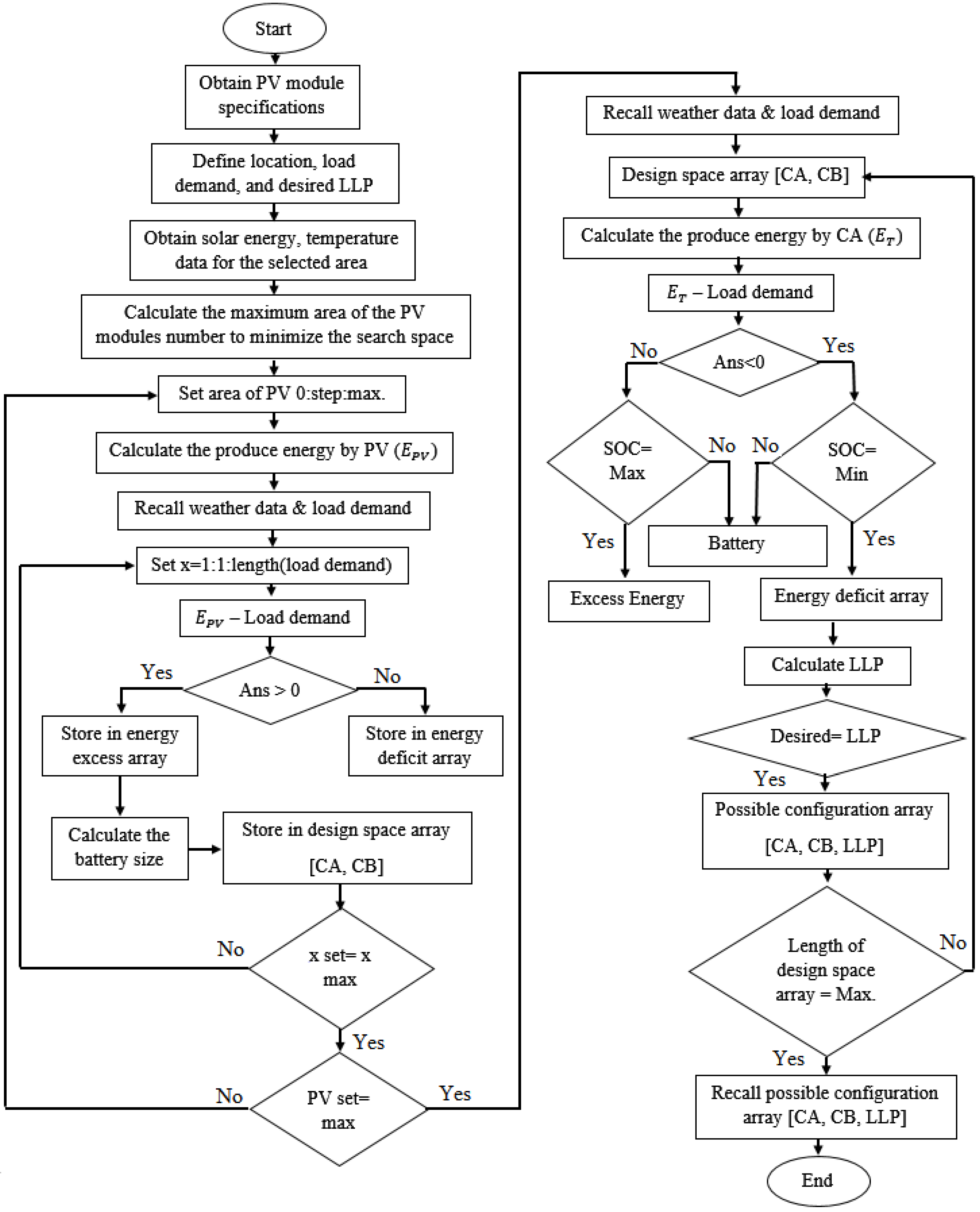
3. Numerical Method for Sizing a Standalone PV System

The sizing criteria of a standalone PV system must take into consideration one of the availability indices. These indices must be calculated for each PV/battery combination in the design space to find the possible PV/battery combinations that satisfy the desired availability index. After that, an objective function is formulated in order to find the optimum size of the PV array and capacity of the battery.

In this research, the system’s availability is calculated using the loss of load probability (LLP). LLP expresses the ability of the system to satisfy the load demand. When the LLP is 0%, this means that the system is able to meet the load demand totally in a specific period without interruption. However, when the LLP is equal to 100%, it means that system is not able to meet the load demand in a specific time at all. In the meanwhile, LLP is defined as the sum of the total energy deficit over the sum of the total load demand during a particular time period, which can be calculated as [13]:

$$LLP=\frac{{\sum }_t^{T}DE\left(t\right)}{{\sum }_t^T{P}_{load}\left(t\right)\Delta t}$$

(21)

where $DE\left(t\right)$ represents the deficit energy term which is the negative energy difference between the generated energy by the PV array and the consumed energy by the defined load at a particular time period, $P_{load}\left(t\right)$ represents the consumed energy by the defined load at the same time period, and $\Delta t$ is the length of the aimed time period.

On the other hand, annualized total life cycle cost ($ATLCC$) is used to estimate the annual costs of the standalone PV system’s components. The $ATLCC$ of a system ($/year) can be mathematically formulated as [17]:

$$ATLCC=C_{cap,other,a}+\frac{{\sum }_{i=1}^{N,pv}i\left(C_{PVi}+L_s{M}_{PVi}\right)}{L.T_{PV}}+\frac{{\sum }_{j=1}^{JBat}j{C}_{Batj}\left(1+Y_{Batj}\right)+M_{Batj}\left(L_s-Y_{Batj}\right)}{L.T_{Bat}}+\frac{{\sum }_{m=1}^{M,chc}m{C}_{chcm}\left(1+Y_{chcm}\right)+M_{chcm}\left(L_s-Y_{chcm}\right)}{L.T_{chc}}+\frac{{\sum }_{u=1}^{U,inv}u{C}_{Inv}\left(1+Y_{Inv})+M_{Inv}(L_s-Y_{Inv}\right)}{L.T_{Inv}}-C_{S,a}$$

(22)

$$C_{cap,other,a}=\frac{\sum C_{cap,other,p}}{\frac{{\left(1+ndr\right)}^{L_s}-1}{ndr{\left(1+ndr\right)}^{L_s}}}$$

(23)

$$C_{S,a}=\frac{C_{S,f}ndr}{{\left(1+ndr\right)}^{L_s}-1}$$

(24)

$$ndr=\left[\left(\frac{1+interst\%}{1+inflation\%}\right)-1\right]$$

(25)

where $C_{cap,other,a}$ represents the annualized capital cost value of the other components and/or related construction works, $C_{cap,other,p}$ represents the present capital cost value of the other components and/or related construction works, $C_{S,a}$ represents the annualized salvage value of the system, $C_{S,f}$ represents the salvage cost value of the system, $ndr$ represents the net of discount-inflation rate [18], $Npv$ represents the number of PV modules in the proposed system, $C_{PVi}$ represents the capital cost value of each PV module, $L_s$ is the operational period of the system’s components, $M_{PVi}$ represents the maintenance cost value per year for each PV module, $L.T_{PV}$ represents the total lifetime period of the PV modules in the system, $JBat$ represents the total number of the batteries in the proposed system, $C_{Batj}$ represents the capital cost value of each battery, $Y_{Batj}$ represents the expected replacement numbers of the batteries during the operational period of the system, $M_{Batj}$ represents the maintenance cost value per year for each battery in the system, $L.T_{Bat}$ represents the total lifetime period of the batteries in the system, $Mchc$ represents the total number of the charge controllers in the proposed system, $C_{chcm}$ represents the capital cost value of each charge controller in the system, $Y_{chcm}$ represents the expected replacement numbers of the charger controller during the operational period of the system, $M_{chcm}$ represents the maintenance cost value per year for each charge controller in the system, $L.T_{chc}$ represents the total lifetime period for the charge controller in the system, $Uinv$ represents the total number of the inverters in the proposed system, $C_{Inv}$ represents the capital cost value of each inverter in the system, $Y_{Inv}$ represents the expected replacement numbers of the inverter during the operational period of the system, $M_{Inv}$ represents the maintenance cost value per year of each inverter in the system, and $L.T_{Inv}$ represents the total lifetime period for the inverter in the system.

In addition, the levelized cost of energy (LCE) is used to find the cost value of the unit generated of energy by the system, LCE

can be mathematically formulated as [19,20]:

$$LCE=\frac{ATLCC}{E_{tot}}$$

(26)

where $ATLCC$ is the annualized total life cycle cost value of the system’s components, and $E_{tot}$ represents the total annual generated energy by the system.

In this research, a standalone PV system is optimally sized using a numerical method based on two battery models, namely, a simple model and a complex model. The sizing algorithm procedure is illustrated in Figure 2. The size optimization algorithm starts with setting the system’s components specifications such as the efficiencies of the PV module, the inverter, the wires, and the charging battery. Load demand and the desired LLP is set and then a series of hourly metrological variables are obtained. To minimize the numerical algorithm’s search space, a range of PV array area is set. For each value of the PV array area, hourly PV array energy output is generated using Equation (4). Then, the energy difference is calculated using Equation (23). During the calculation of the energy difference, matrices of energy excess and energy deficit values are created. From the excess and deficit matrices, the capacity of the storage battery is obtained. This loop is repeated until it reaches the maximum range of the PV array area. After that, the battery capacities and the PV array sizes matrix is constructed. Here, an hourly energy flow model is implemented to find the LLP value for each PV/battery combination. The hourly energy flow model is operated based on two cases which are depending on the value of energy difference ($E_D\left(t\right)$) in order to calculate the LLP value of each combination. The first scenario is when $E_D\left(t\right)>0$. The case happens when $E_{PV}\left(t\right)$ is more than the $E_L\left(t\right)$.

In this case, the load demand is totally covered by the PV array while an amount of excess energy will result. The amount of excess energy flow is depending on the instantaneous SOC of the battery. If the battery is fully charged ($SOC=SO{C}_{max}$), all of excess energy amount will be stored in the excess energy matrix. Otherwise, the amount of excess energy is used to charge the battery. Here, the battery is charged and the new value of SOC is calculated using Equation (25). In this case, there is no energy deficit. The second scenario (($E_D\left(t\right)<0$) shows the case when $E_{PV}\left(t\right)$ is less than the $E_L\left(t\right)$. In this case, the energy produced by the PV array is insufficient to meet the load demand. Therefore, the battery must supply the load. In this case, if the $SOC=SO{C}_{min}$, the PV system and the battery are not able to meet the load demand. Therefore, the amount of energy deficit is equal to the load demand. Otherwise, the battery is able to supply the load demand. This loop is repeated while the LLP of all the combinations is being calculated. Eventually, all of the combinations that are obtained from the hourly energy flow are nominated based on the desired LLP.

After defining the design space, the annualized total life cycle cost (ATLCC) of each PV/battery combination in the design space is calculated. Finally, the best combination which achieves the minimum ATLCC is selected.

In the second optimization algorithm, the same optimization process is applied but considering the complex battery models represented by Equations (6–20).

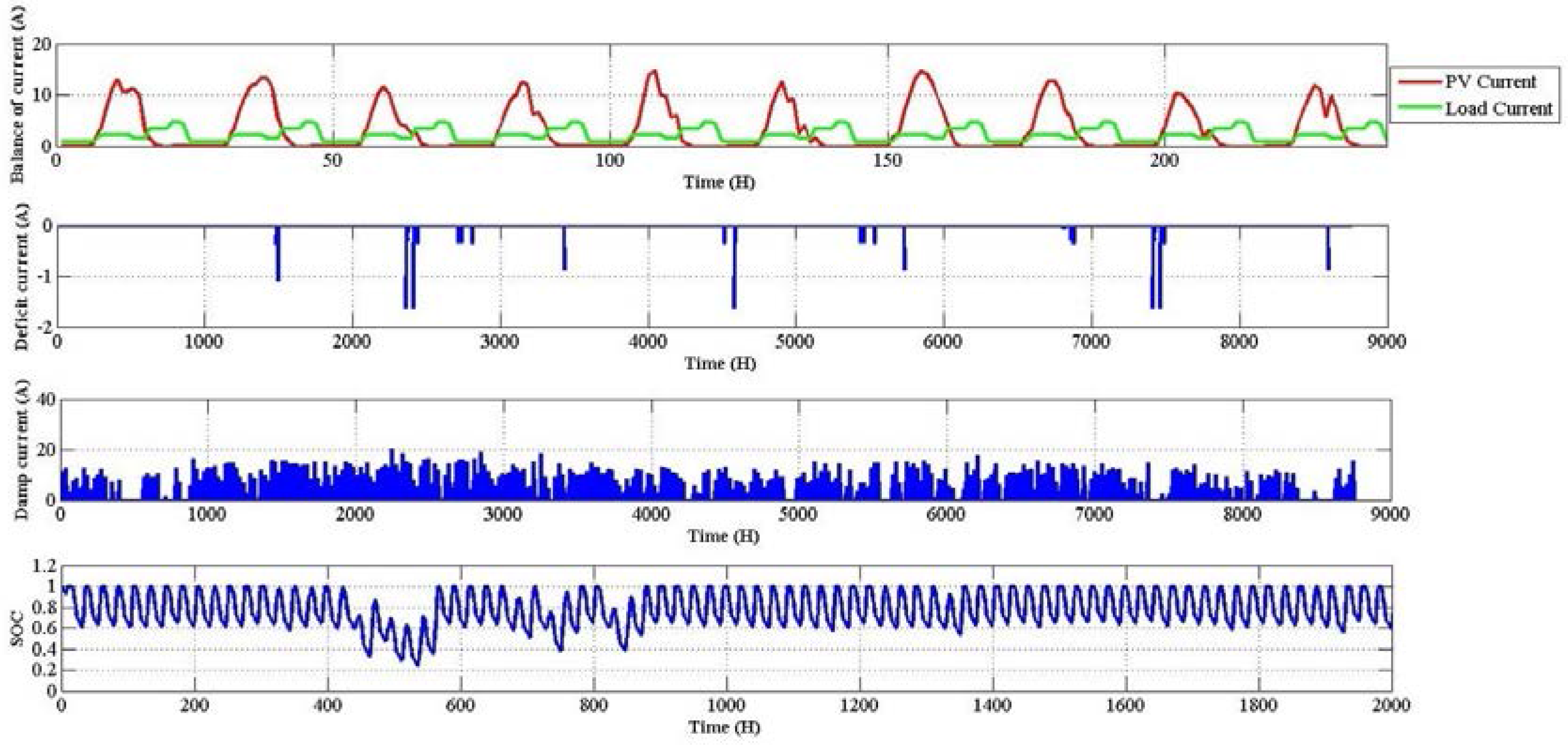
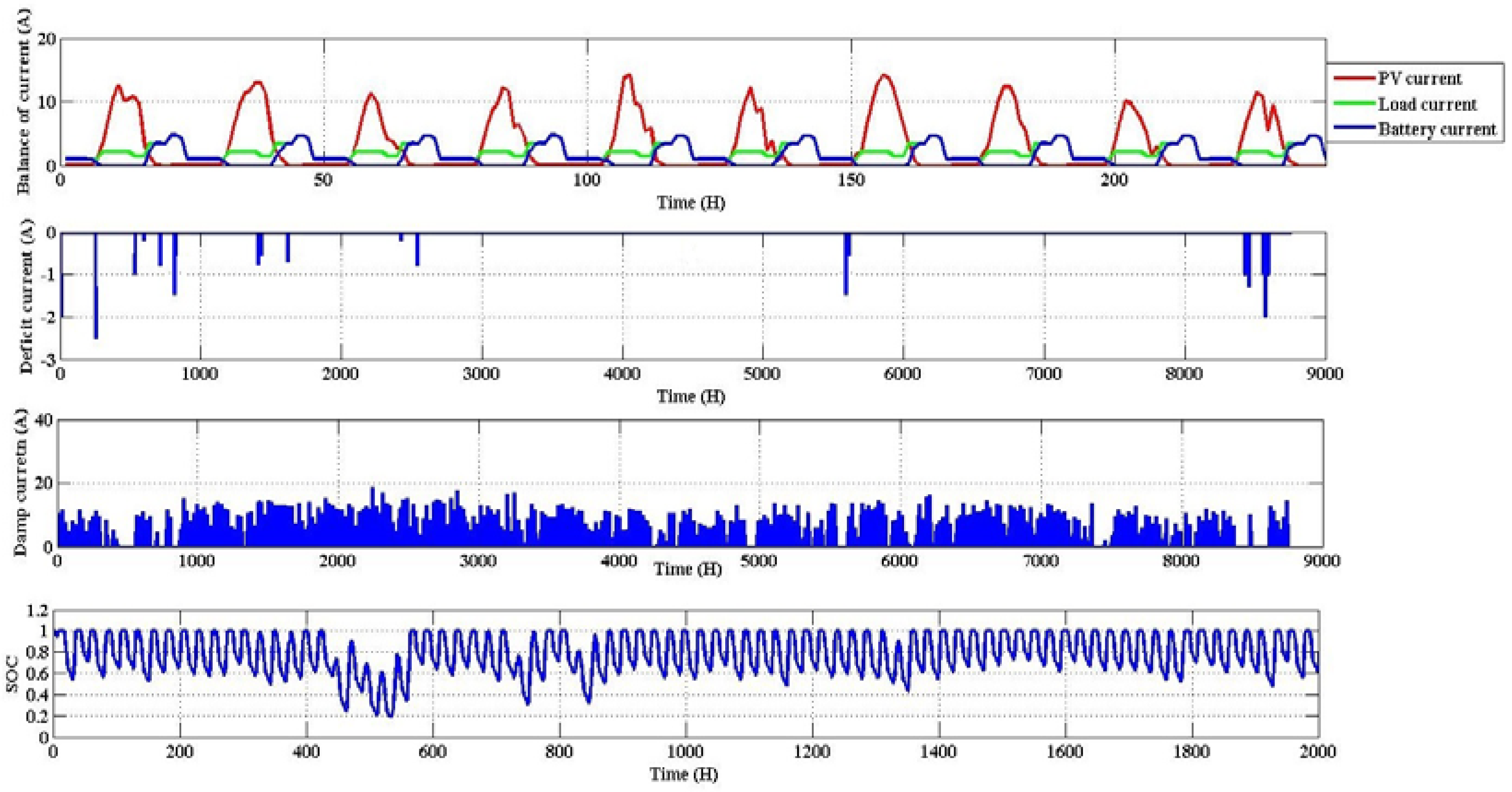
4. Results and Discussion

The size optimization process in this research is done based on Malaysian’s metrological data. Hourly metrological data for one year in Klang Valley, Malaysia are used in the optimization processes. Based on these data, the annual daily averaged solar radiation is 362.52 $W/m^2$, with the best value in March (427.6293 $W/m^2$) and worst value in December (314.9887 $W/m^2$).

In this research, daily load demand data of a typical house in a rural area in Malaysia are used in the both size optimization algorithms as it is illustrated in Figure 3. The annual daily averaged load demand is 12.305 kWh/day (1.081 kW peak). In this research, the proposed standalone PV system is supposed to supply the load demand subject to 1% LLP.

In addition to that,

Table 1. Electrical characteristics of the adopted system at $STC$.

Module Type	STF-120P6
Rated Power ($P_{max})$	120 $W$
Open-circuit Voltage ($V_{oc}$)	21.5 $V$
Short-circuit Current ($I_{sc}$)	7.63 $A$
Voltage at MPP ($V_{MP}$)	17.4 $V$
Current at MPP ($I_{MP}$)	6.89 $A$
Nominal Operation Cell Temperature ($NOCT$)	43.6 $℃$
Temperature Coefficient of $I_{sc}$ ($\alpha$)	6.93 $mA/℃$
Temperature Coefficient of $V_{oc}$ ($\beta$)	−0.068 $V/℃$
Temperature Coefficient of $P_{max}$ ($\gamma$)	−0.39$\%$
Dimension of module	(1470 × 662 × 45) $mm$
PV Module Efficiency	14%
Inverter Capacity	3 $kW$
AC Voltage	230 $V$
Inverter efficiency	95%
Nominal Battery Voltage	12 $V$
Rated Capacity of the Battery	100 $Ah$
Battery Discharging efficiency	80%
Max. allowed Depth of Discharged	80%
Max. Discharged current (25$℃$)	800 A
Min. $SOC$ of the battery	20%

and

Table 2. Costs of the system’s components for the adopted system.

Cost code	Standalone PV system’s items	Unit cost ($)
1	PV
1.1	Capital Cost	3.8/Wp
1.2	Maintenance Cost	0.0542/Wp/year
2	Battery
2.1	Capital Cost	4.8/Wh
2.2	Maintenance Cost	0.003/Wh/year
2.3	Replacement	0.042/Wh/years
3	Charge controller
3.1	Capital Cost	400/charge controller
3.2	Maintenance Cost	0
4	Inverter
4.1	Capital Cost	800/Inverter
4.2	Maintenance Cost	0
5	Other Costs
5.1	Circuit Breaker	25/Circuit Breaker
5.2	Support Structure	200
5.3	Civil work	400
6	Salvage Value	14% of total NPV cost
7	Discount rate (%)	3.5%
8	Inflation rate (%)	1.5%
9	NDR (%)	1.97%
10	Number of years	25 years

show the adopted system’s specifications and cost components, respectively.

In order to highlight the importance of the system’s battery model on the results of the optimization process, the results of the complex battery model are compared with the results obtained based on the simple battery model using the same case study’s metrological data, load demand, and system specifications. Figure 4 show the PV array size and the storage battery capacity at an LLP of 0.01 using simple and complex battery models, respectively.

According to the results, the minimum PV/battery combination’s total life cycle cost for method 1 is 6598.7$/year. The optimum size combination of the PV array and storage battery are 4.32 kWp, and 1668.1 Ah/12 V, respectively. On the other hand, based on method 2, which considers the complex battery’s model, the optimum PV/battery combination’s total life cycle cost is 4556.9$/year. While the optimum size combination of PV array and storage battery are 4.08 kWp and 1168.1 Ah/12 V, respectively.

In order to make a comparison between the two proposed methods, the systems’ simulation is conducted as shown in Figure 5 and Figure 6.

According to the results of the first system, the PV array produced 6382.2 kWh per year, while the battery supplies the load by about 4298 kWh per year. In addition, the levelized cost of energy (LCE) for unit generated by this system is 0.618$/kWh with an actual value of LLP of 0.0097. Meanwhile, in the second system, the PV array produces 6027.4 kWh per year, while the battery supplies the load by about 2973 kWh per year. However, the LCE by this system is about 0.505$/kWh with an actual value of LLP is 0.0095. To sum up all the differences in results for the both models,

Table 3. Comparison of differences in results for the both methods.

Items	Method 1	Method 2
PV array size	4.32 kWp	4.08 kWp
Battery capacity	1668.1 Ah/12 V	1168.1 Ah/12 V
PV array energy produces/year	6382.2 kWh/year	6027.4 kWh/year
Battery energy supplies/year	4298 kWh/year	2995 kWh/year
Energy deficit	0.1194 kWh/day	0.1169 kWh/day
Excess energy	5.1963 kWh/day	3.4825 kWh/day
Actual LLP	0.0097	0.0095
Total life cycle cost	6598.7$/year	4556.9$/year
LCE	0.618$/kWh	0.505$/kWh

highlights these differences.

From these results, it is clear that the algorithm which is based on the complex battery model resulted smaller system size as compared to the algorithm that is based on the simple battery model. The complex battery model reflected more accurate behavior of the storage battery which reduced the needed amount of the energy from storage battery to supply the load demand that decreases the capacity of the battery. Consequently, the cost of the system is greatly affected. This is to say that in order to get accurate optimization results, accurate modeling of the battery is needed.

5. Conclusions

A comparative study between two proposed size optimization methods for a standalone PV system based on two battery models was presented. The complex model of a battery utilized in this research gave better results than the optimization done based on the simple battery model. There is a significant difference between the PV array capacity calculated using method 1 and method 2. The PV array capacity in method 2 is 4.08 kWp, which is less than the PV array capacity calculated using the method 1 by 5.6% (4.32 kWp). On the other hand, the storage battery capacity in method 2 is 1.1681 kAh, which is less by 30% than that calculated using method 1, which is 1.6681 kAh. The main factor that causes the differences in the PV array and storage battery sizes is the dynamic battery model, which incorporates the dynamic behavior of the battery especially during the discharge process, which is accurately calculating the SOC of the battery. The total life cycle cost in method 2 (4556.9 $/year) is reduced by 31% according to the total life cycle cost calculated using method 1 (6598.7 $/year). Meanwhile, the cost of the generated unit of energy in method 2 (0.506$/kWh) is less than that calculated using method 1 by 18.1% (0.618$/kWh). Thus, method 2 is more accurate and cost-effective than method 1 with the same range in the level of availability (0.0095–0.0105).

References

1. Masters, G.M. Renewable and Efficient Electric Power Systems, 2nd ed.; John Wiley & Sons, Inc.: Hoboken, NJ, USA, 2013. [Google Scholar]
2. Khatib, T.; Ibrahim, I.A.; Mohamed, A. A review on sizing methodologies of photovoltaic array and storage battery in a standalone photovoltaic system. Energy Convers. Manag. 2016, 120, 430–448. [Google Scholar] [CrossRef]
3. Thevenard, D.; Pelland, S. Estimating the uncertainty in long-term photovoltaic yield predictions. Sol. Energy 2013, 91, 432–445. [Google Scholar] [CrossRef]
4. Shen, W.X. Optimally sizing of solar array and battery in a standalone photovoltaic system in Malaysia. Renew. Energy 2009, 34, 348–352. [Google Scholar] [CrossRef]
5. Khatib, T.; Mohamed, A.; Sopian, K.; Mahmoud, M. A new approach for optimal sizing of standalone photovoltaic systems. Int. J. Photoenergy 2012, 2012, 1–7. [Google Scholar] [CrossRef]
6. Nordin, N.D.; Rahman, H.A. A novel optimization method for designing stand alone photovoltaic system. Renew. Energy 2016, 89, 706–715. [Google Scholar] [CrossRef]
7. Abbes, D.; Martinez, A.; Champenois, G. Life cycle cost, embodied energy and loss of power supply probability for the optimal design of hybrid power systems. Math. Comput. Simul. 2014, 98, 46–62. [Google Scholar] [CrossRef]
8. Khatib, T.; Mohamed, A.; Sopian, K. A review of photovoltaic systems size optimization techniques. Renew. Sustain. Energy Rev. 2013, 22, 454–465. [Google Scholar] [CrossRef]
9. Bhuiyan, M.; Asgar, M. Sizing of a stand-alone photovoltaic power system at Dhaka. Renew. Energy 2003, 28, 929–938. [Google Scholar] [CrossRef]
10. Li, C.-H.; Zhu, X.-J.; Cao, G.-Y.; Sui, S.; Hu, M.-R. Dynamic modeling and sizing optimization of stand-alone photovoltaic power systems using hybrid energy storage technology. Renew. Energy 2009, 34, 815–826. [Google Scholar] [CrossRef]
11. Abido, M.A. Multiobjective particle swarm optimization for environmental/economic dispatch problem. Electr. Power Syst. Res. 2009, 79, 1105–1113. [Google Scholar] [CrossRef]
12. Ameen, A.M.; Pasupuleti, J.; Khatib, T. Simplified performance models of photovoltaic/diesel generator/battery system considering typical control strategies. Energy Convers. Manag. 2015, 99, 313–325. [Google Scholar] [CrossRef]
13. Kazem, H.A.; Khatib, T.; Sopian, K. Sizing of a standalone photovoltaic/battery system at minimum cost for remote housing electrification in Sohar, Oman. Energy Build. 2013, 61, 108–115. [Google Scholar] [CrossRef]
14. Chen, S.-G. An efficient sizing method for a stand-alone PV system in terms of the observed block extremes. Appl. Energy 2012, 91, 375–384. [Google Scholar]
15. Kaldellis, J.K.; Zafirakis, D.; Kondili, E. Optimum sizing of photovoltaic-energy storage systems for autonomous small islands. Int. J. Electr. Power Energy Syst. 2010, 32, 24–36. [Google Scholar] [CrossRef]
16. Castañer, L.; Silvestre, S. Modelling Photovoltaic Systems Using PSpice; John Wiley & Sons Inc.: West Sussex, UK, 2002. [Google Scholar]
17. Mohamed, A.F.; Elarini, M.M.; Othman, A.M. A new technique based on Artificial Bee Colony Algorithm for optimal sizing of stand-alone photovoltaic system. J. Adv. Res. 2013, 5, 397–408. [Google Scholar] [CrossRef] [PubMed]
18. Bull, J. Life Cycle Costing for Construction; Routledge: New York, NY, USA, 2003. [Google Scholar]
19. Yang, H.; Lu, L.; Zhou, W. A novel optimization sizing model for hybrid solar-wind power generation system. Sol. Energy 2007, 81, 76–84. [Google Scholar] [CrossRef]
20. Lazou, A. A.; Papatsoris, A.D. Economics of photovoltaic stand-alone residential households: A case study for various European and Mediterranean locations. Sol. Energy Mater. Sol. Cells 2000, 62, 411–427. [Google Scholar] [CrossRef]
Figure 1. Equivalent electrical circuit of the lead-acid battery.
Sustainability 08 00894 g001
Figure 2. The size optimization algorithm for determining the design space at desired LLP in [13].
Sustainability 08 00894 g002
Figure 3. Daily load demand of a typical house in rural area in Malaysia.
Sustainability 08 00894 g003
Figure 4. (a) Design space for the proposed standalone PV system model at 0.01 LLP using a simple battery model (method 1); (b) Design space for the proposed standalone PV system model at 0.01 LLP using a complex battery model (method 2).
Sustainability 08 00894 g004
Figure 5. Current generation share, damping and deficit currents, and battery SOC based on the first method.
Sustainability 08 00894 g005
Figure 6. Current generation share, damping and deficit currents, and battery SOC based on the second method.
Sustainability 08 00894 g006