Abstract
What factors determine the spatial heterogeneity of household energy consumption (HEC) in China? Can the impacts of these factors be quantified? What are the trends and characteristics of the spatial differences? To date, these issues are still unclear. Based on the STIRPAT model and panel dataset for 30 provinces in China over the period 1997–2013, this paper investigated influences of the income per capita, urbanization level and annual average temperature on HEC, and revealed the spatial effects of these influencing factors. The results show that the income level is the main influencing factor, followed by the annual average temperature. There exists a diminishing marginal contribution with increasing income. The influence of urbanization level varies according to income level. In addition, from the eastern region to western region of China, variances largely depend upon economic level at the provincial level. From the northern region to southern region, change is mainly caused by temperature. The urbanization level has more significant impact on the structure and efficiency of household energy consumption than on its quantity. These results could provide reference for policy making and energy planning.
1. Introduction
Household energy consumption (HEC) accounts for 35% of total energy end-use worldwide. In China, its share is 10.6% [1]. HEC will further increase by rapid economic growth and urban transformation in China [2,3]. At present, China’s economy is entering the “new normal”, maintaining economic growth above 6.5%. Meanwhile, China is one of the most rapidly urbanizing countries in the world with the urbanization rate of 17.9% in 1978 and 54.77% in 2014. The average annual urbanization rate is 1%. It is predicted this rate will reach approximately 70% by the end of 2030 [4]. However, excessive consumption of fossil fuels is the major cause of global warming and air pollution, which becomes the greatest challenge to sustainable development [5]. There are many studies on response to the challenge [6], in which few reports are from the view of spatial variances.
Energy consumption is one of the most fundamental needs for peoples’ lives, which is closely related to all aspects of social activity. HEC, as the energy end-use, becomes the standard by which people’s quality of life is measured [7]. There are many factors influencing HEC, including climatic conditions, income levels, cultural traditions, lifestyle of residents, and so on. Thus, there is a huge variation in the quantity, structure, pattern and greenhouse gas (GHG) emissions of the fuel consumed by households. The existing literature has investigated the impacts of people’s income [8,9], geographical conditions [10,11], fuel prices [9,12], household demographic characteristics [3,13], etc. on HEC. Many articles discussed the relationship between the energy use in household sector and various affecting factors from different regional scales, for example, county [14], city [15], and province [16]; urban and rural areas [17,18]; and agricultural and pastoral zones [19]. Obviously, the aims of these studies are not to reveal the spatial difference in domestic fuel use.
Other literature probed the spatial effects of GHG emissions and spatial variation of energy consumptions [20,21,22], but there were no deep discussions on influence factors. In addition, Jiang and Ji applied a spatial Durbin model to test for spatial spillover effects among energy intensity and seven exogenous variables, and offer some theoretical evidence for differential localized energy policy [23]. Nevertheless, they investigated the spatial difference of whole energy consumption rather than that in a sector.
What factors have important impacts on the spatial heterogeneity of HEC in China? What are the trend and characteristics of the spatial differences? Can these impacts be quantified? To date, these issues are still unclear. Therefore, to address these knowledge gaps can help us deeply understand the change mechanisms of HEC [24], optimize energy planning and environmental governance policies.
China has great geographical difference. Energy and mineral resources are mainly distributed in the western and northern regions, and population and industrial production are concentrated along the southeast coast. Thus, the energy supply does not match the energy demand in the geographical space [25]. A huge geographical difference and imbalance of social-economic development make spatial variances of HEC have more performance in China. In addition, the lifestyle of the urban resident is significantly different from that of rural resident in the same geographical area, leading to corresponding differences in HEC and environmental effect [21]. Thus, it is necessary to investigate the variations between urban and rural areas.
The aim of this paper is to reveal the main factors influencing HEC on a macro scale and the trend of their spatial variance in China, measure quantitatively the effect intensity of these factors, and deepen the understanding of the spatial association between geographical, social, and economic factors and HEC. In addition, the public policy regarding energy governance is discussed. The rest of the paper is organized as follows. Section 2 presents the literature review on influencing factors of HEC. Section 3 presents STIRPAT model and data sources. In Section 4, empirical results are analyzed. Section 5 provides discussion and conclusions.
2. The Literature Review
The energy use in household sector is influenced by many factors, which can be summarized as three aspects: physical geography, economic development, and social transformation. Some factors are mixed, such as urbanization. Based on many methodologies, the existing literature analyzed the relationship between HEC and various factors, and revealed their interactions and change trend. The relevant literature is summarized in Table 1.

Table 1.
The summary of relevant studies on energy consumption in household-sector.
2.1. Geographic Factors
Human survival and development highly depend on natural environments. Many geographic factors, including climate, terrain, vegetation, energy and mineral resources endowment, etc., influence HEC. Among them, climate condition plays the most important role on fuel use. It is difficult for humans to withstand ambient temperatures below 0 °C or above 30 °C [26]. Thus, they need to keep cool in hot weather and warm in cold weather by controlling indoor temperatures. Temperature varies with the latitude and elevation. In high latitude regions, temperature is normally less than 5 °C in the winter, and local inhabitants need space heating. In low latitude regions, temperature is normally greater than 30 °C in the summer, and local inhabitants need space cooling. The impact of the elevation on temperature is similar with that of the latitude. The energy for heating and cooling accounts for large proportion of total HEC; this share is 58% in the US [10], and 67% in China [27]. The relationship between HEC and temperature has received growing attention during the last three decades. Sun presented the linear relationship between annual per capita energy consumption and annual average temperature in 29 regions of China in 1990 [28]. Henley et al. showed the non-linear link between electricity consumption and temperature in 15 European countries [29,30]. Considine et al. suggested that warm climate slightly reduced energy consumption and carbon emissions in the US [11,31]. The results of Mirasgedis et al. indicated an increase in the annual electricity consumption attributable solely to climate change of 3.6%–5.5% under all examined scenarios [32].
The most common climatic indicator of the demand for heating and cooling services is the degree day: heating degree days (HDD) are the period of air temperature (Tm) > 18 °C, and cooling degree-days (CDD) are the period of Tm < 18 °C [33]. Temporal downscaling, using monthly, daily or at best hourly data, increases the accuracy of examining the relationship between energy consumption and temperature [34]. For instance, Ruth and Lin [31] use monthly data; Henley and Peirson [29] use daily data; and Parkpoom and Harris [35] use hourly data. However, it is difficult to obtain monthly, daily and hourly data on household energy consumption.
2.2. Economic Factors
The income level is taken as a basic variable in almost all literature on HEC. It is not only an indicator of economic development level of regions or countries, but also a reflection of household paying ability (Table 1). In developing countries, such as Vietnam [36], India [37] and China [1,9], the household income is the key factor affecting quantity and structure of energy use.
Some studies apply GDP per capita to explain and variation in emissions across stages of development, and results indicate that there is a positive relationship between them [37,38,39,40]. The energy price is one factor affecting household energy consumption, which has a negative impact. Increasing prices may discourage HEC in the US [13]. Cheap electricity prices may hamper the development of energy-saving implementations in household sector in China [1]. Moreover, electricity consumption and household electrical appliances use are heavily interdependent. Niu et al. found that the impact of appliance prices on power consumption is much greater than that of electricity prices [9]. Nie and Kemp (2014) argued that the increase in energy-using appliances is the biggest contributor to the increase of residential energy use [41].
2.3. Social Factors
In addition, some social factors also affect HEC. The demographic characteristics have clear effects on energy consumption; population increases are matched by proportional increases in energy use and emissions [13]. Changes in age structure of population have impact on energy consumption [42]; for example, older people probably consume more energy than younger people [43]. The number of household members is a significant explanatory variable. A large family usually consumes more energy than a small family, but energy consumption per capita is less than that of a small family [9,44]. In addition, rural to urban migration shows a significant and negative influence on HEC and CO2 emissions [36].
The impact of lifestyle on energy use mainly reflects types and purposes of fuels chosen by different households. China is a country with typical binary economics and social diversity, and there is a significant difference in the consumption pattern between urban and rural regions [45]. Urban residents consume high-quality energy, such as electricity, natural gas, heating power, solar energy and gasoline. For rural residents, besides electricity, coal and biomass are used, which require much time and labor, and are heavy indoor pollutants [46]. The difference in energy consumption pattern between urban and rural residents is closely related to dwelling attributes and energy public infrastructure [9,47]. Compared with rural households, urban households, usually living in multistory buildings, easily access clean and effective fuels through the electric grid, natural gas network and district heating system [37,48]. Therefore, we regard urbanization level as an integrated variable reflecting social progress situation.
In fact, the above factors are interdependent, and they simultaneously influence HEC. Many scholars regard the urbanization process as a comprehensive variable to analyze the issue on energy use in household sector (Table 1). Some results indicate that urbanization increases the number of energy utilization through changes in lifestyles, which means there is a positive relationship between urbanization and household energy consumption [42,51,53,55,57,65,71]. However, some studies provide the opposite result [34,42,67]. Other studies show some mixed results, indicating that the relationship between urbanization and household energy use is complex and remains inconclusive [38,40]. The disagreement in the existing studies can be attributed to differences in methodologies, data and stages of development [38,40,56]. However, there is a common feature: the structure of energy use shifts from inefficient solid fuels in rural areas to more efficient commercial fuels in urban areas [7,37,60,72,73].
Therefore, the combination effect of these factors should be considered at national scale for drawing the accurate and detailed characteristics of the HEC in China, and this consideration could provide valuable insights to develop flexible and practical energy conservation and emission reduction policies against the environmental issues in China.
3. Methodology and Data
3.1. The STIRPAT Model and Panel Data Model
There are many mathematical models used to research the relationship between HEC and its influencing factors (Table 1). Among them, the STIRPAT (Stochastic Impacts by Regression on Population, Affluence and Technology) is the most widely applied model [52], which was proposed by Dietz and Rosa in 1994 [74] to overcome the limitations of the IPAT model (I = PAT) [57]. The pivotal limitation of IPAT is that it does not permit hypothesis testing because known values of some terms determine the value of the missing term [75]. Moreover, the IPAT model does not isolate the most important driver behind the identified environmental impacts [57]. The STIRPAT model may overcome these limitations, so it has been increasingly used to investigate the interaction between socio-economic changes and the environment. The model is as follows:
where α is the constant term. b, c and d are elasticities of environmental impacts of P (population size), A (affluence) and T (technology), respectively. The variable e denotes the error term, and the subscript i represents the region where the analysis has been made, such as a province.
There are great differences in population, land area and level of economic development among 30 provinces (or municipalities and autonomous regions) in China. To compare the spatial variances among provinces, we take per capita energy consumption in household sector as the explained variable, which is equivalent to move P from the right side of the Equation (1) to the left side (). After taking natural logarithms of both sides of STIRPAT model, the empirical model for the panel data can be written as follows:
where GDP is measured by the GDP per capita (thousand Yuan), URB denotes the urbanization level (percent), TEM denotes annual average temperature (°C), e1it denotes random disturbance term for Equation (2). Enp represents energy consumption per capita (kgce) in the household sector in China, αi is the elasticity coefficient.
In order to differentiate urban and rural areas, we use per capita income instead of GDP per capita and a dummy variable instead of the urbanization level. Then, the estimation of the difference between urban and rural areas in household energy use is conducted with Equation (3).
where D presents a dummy variable to distinguish rural and urban areas, and e2it denotes random disturbance term for Equation (3).
We employ 13 different panel data models to estimate parameters. Panel data analysis help us to full use of the information contained in the samples and reflect the changing trends of research objects in three dimensions (cross-section, period and variables) [57,76]. These methods include: (1) the pooled Ordinary Least Squares (OLS); (2) fixed effects (FE); (3) hetonly and two-way fixed effects (Two-way FE); (4) the corrected Least Square Dummy Variables (FE-LSDV); (5) the first difference estimates (FD); (6) Random effects (RE); (7) LM test for individual-specific effects (RE-ML); (8) the linear regression with panel-corrected standard errors (PCSE); (9) the linear regression with Driscoll–Kraay standard errors (DK); (10) the feasible generalized least squares (FGLS); (11) Prais–Winsten (PW); (12) two step of Generalized Method of Moment (2S-GMM); and (13) Dynamic panel data.
3.2. Hypotheses
H01: there is the spatial heterogeneity in HEC, which means that the intercept term and coefficient of explanatory variables in Equation (2) vary across provinces, , . In addition, the spatial difference shows the consistency of space.
H02: there is a difference between urban and rural areas in HEC per capita, which implies that the coefficients of dummy variable D (D = 1 in urban area, D = 0 in rural area) would be great or statistically significant in Equation (3). Because the temperatures of the same province are invariable, energy consumption is entirely determined by resident income.
3.3. Data Source
This study uses a balanced panel data of 30 provinces in China (excluding Tibet, Hong Kong, Macao and Taiwan) covering the period from 1997 to 2013. The provincial data on household energy use are derived from annual China Energy Statistical Yearbook (1998–2014) [77]. The data on GDP per capita, per capita income (per capita disposable income of urban residents and per capita net income of rural dwellers) and urbanization level are mainly obtained from annual China Statistical Yearbook (1998–2014) [78]. In addition, the GDP per capita is calculated by the constant prices of 2000 (thousand Yuan, RMB). The data of provincial average temperature come from National Meteorological Information Center [79].
It is important to note that energy source used in rural areas does not include bio-fuels, which is not calculated by official statistics [28]. It only contains commercial energy in annual China Energy Statistical Yearbook.
4. Empirical Results
4.1. Impacts of Several Factors on Household Energy Consumption
4.1.1. Effect of Economic Growth
The results of the panel unit root tests show that the first-order difference series of all variables, except PP test of LnGDP, are stationary (Appendix A). Using Stata 14 soft, we conduct parameter estimation for 13 different models. Results show that GDP per capita, which represents a region’s economic development level, has a significant positive impact on household energy consumption of all models (Table 2). About two-way fixed effects (Two-way FE) model, lnGDP has high elasticity of 1.691 because of the annual dummy variables with negative time effects (Appendix B). For dynamic panel data (DPD) model, there is the lagged term of dependent variable lnEnp with the coefficient of 0.827, which reflects the inertial effect of HEC, so the elasticity of lnGDP decreases to 0.155. For other models, the elasticities of lnGDP are between 0.49 and 0.865 with small variations. It is indicated that a 1% increase in GDP per capita (thousand Yuan) would lead to 0.75% (it is a mean value of 13 elasticities of lnGDP) increase in energy consumption per capita (kgce) when other factors remain constant. China’s GDP per capita rapidly increased from 7902 Yuan (constant 2000) in 1997 to 25,386 Yuan in 2013. It has more than tripled during the past 17 years, and becomes a main factor driving the energy consumption.
Table 2.
Estimation results for parameter of 13 different models for whole sample (n = 30).
4.1.2. Effect of Urbanization Process
There are 11 negative values and two small positive values in 13 elasticity coefficients of lnURB (Table 2). Among them, five coefficients are significant at p < 0.01 level, two coefficients are significant at p < 0.1 level, and another six coefficients are not significant. Furthermore, China’s urbanization rate increased from 31.9% in 1997 to 53.7% in 2013, which is a rapid growth rate from the view of urbanization process. However, compared with the economic growth rate, it is low. This indicates that the influence of urbanization on household energy consumption is far less than that of GDP per capita, which is consistent with the argument that changes in urbanization have a somewhat less than the proportional effect on aggregate energy use [60]. The negative elasticities indicate that a 1% increase in urbanization level would decrease household energy use per capita by 0.54% (it is a mean value of seven elasticities of lnURB that are statistically significant). Our results are different with some previous studies that show urbanization increases energy consumption [57,71,72], and are supported by other studies [37,40,50,68]. The reason could be that urbanization encourages fuels switching from inefficient traditional fuels to modern fuels, which are more efficient, leading to energy saving [38,56].
Impacts of urbanization on energy consumption are mixed in the existing studies and vary across the stages of development when it is applied in more countries [56]. Li and Lin [38], Chikaraishi et al. [52], Poumanyvong et al. [56], and Poumanyvong and Kaneko [40] employed 73, 140, 88 and 99 countries to investigate the issue, respectively. Their results are similar: urbanization decreases household energy use in low-income countries, while it increases energy use in high-income countries. Table 3 shows estimated results for the less developed western region (11 provinces) except dynamic panel data model, elasticities of lnURB are negative and significant at p < 0.1 level. In the relatively developed eastern region (19 provinces), which equates with middle-income countries worldwide, there are four positive and nine negative coefficients (Table 4). It shows the characteristic of the transition stage from low to high income. In a nutshell, our results are fairly consistent with international experiences [38,39,52,56]. If we consider urbanization as the result of regional economic growth, and take out variable lnGDP from all models, all elasticities of lnURB will be positive values (Table 5). In this case, the impact of urbanization on household energy use is significant. Actually, there is collinearity between lnGDP and lnURB, these two variables interact closely. Urbanization causes economic output, which in turn pushes urbanization process [80].
Table 3.
Estimation results for parameter of 13 different models in the western region (n = 11).
Table 4.
Estimation results for parameter of 13 different models in the eastern region (n = 19).
Table 5.
Estimation results for parameter of 13 different model without lnGDP (n = 30).
4.1.3. Effect of Temperature Variance
The coefficients of lnTEM are negative for all models (Table 2, Table 3, Table 4 and Table 5), which indicate that a 1% increase in annual average temperature would decrease energy demand per capita by 0.12% to 0.823%. Among them, six, one and two coefficients of these models are significant at p < 0.01 level, p < 0.05 level and p < 0.1 level, respectively, and four other coefficients are insignificant (Table 2). Since temperature variances of 29 provinces in 17 years are less than 0.6 °C, except Chongqing City (0.92 °C), the impact of temperature change on household energy consumption is small in the same region. Territory of China has a large span in latitude and longitude, the annual average temperatures in the southernmost province, Hainan, and the northeast province, Heilongjiang, are 24.6 °C and 5.3 °C, respectively. With the higher elevation, Qinghai Province has the second lowest annual average temperature. The difference in temperatures between provinces is significant (Figure 1). Thus, temperature is a spatial variable, and has a relatively large impact on household energy demand across provinces.
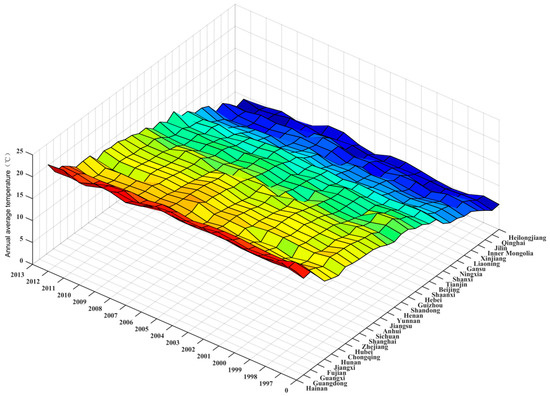
Figure 1.
Annual average temperatures of 30 provinces in China during 1997–2013.
4.2. Spatial Heterogeneity of HEC
4.2.1. Differences between the Eastern and the Western Regions of China
Comparing two coefficients of lnGDP estimated by same model in Table 3 and Table 4, we can find that the coefficient of the western region is always greater than that of the eastern region. Due to , there is the spatial difference in household energy use, which means the hypothesis H01 is true. This indicates that the contribution of GDP per unit to household energy use in the western region is more than that in the eastern region. GDP per capita in the eastern region was two times and 1.8 times of that in the western region in 1997 and 2013, respectively. In addition, the proportion between them declined slowly, but there has been a steady increase in the absolute difference. The east and the west of China have been at different stages of development, and income level is a strong factor that affects spatial variance of household energy consumption in China.
Similarly, when the elasticities of lnTEM are estimated by the same model, results (absolute value) in the western region are still greater than that in the eastern region (Table 3 and Table 4). The coefficients of 12 models except DPD are statistically significant in the western region (Table 3), and only seven models’ coefficients are statistically significant in the eastern region. This indicates that residents living in the western region with high altitude are more sensitive to temperature change in household energy consumption.
4.2.2. Differences between the Northern and the Southern Regions of China
In the northern region of China with high latitude, the cold weather lasts longer than the southern region. The energy consumption for heating is large and relatively inelastic for long time. In recent years, residents in the southern region increase energy use, especially electricity consumption, for cooling in the summer as their incomes rise. The impact of temperature change on household energy consumption shows in the intercept terms of the fixed effect models (Figure 2). Intercepts vary across provinces in models, and this variance shows clear spatial difference between the northern region and the southern region. Then, Equation (2) can be changed as follows:
where is the intercept of the ith province. Most of intercepts are positive in the northern provinces, and the sum of increases; and they are negative in the southern provinces, and the sum of decreases. This indicates that the base of HEC in the northern region is higher than that in the southern region. In addition, annual average temperatures of Guizhou Province and Shandong Province are remarkably close, but intercept of Guizhou Province (in southwest China) is positive, and that of Shandong Province (in northeast China) is negative. They belong to opposite groups. Actually, Guizhou is a mountainous province with high altitude, which has a wide temperature range. Thus, the base of energy consumption is high. However, Shandong Province is located in the plain and adjoins the sea. Thus, small temperature variance leads to low base of energy consumption. In sum, , and there is a spatial difference. Thus, the hypothesis H01 is true.
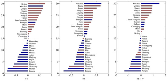
Figure 2.
Intercepts variance across 30 provinces.
4.2.3. Differences between Urban and Rural Areas
As FD, 2S-GMM and DPD (three models) are unsuitable for estimating parameters of virtual variable, we employ the other 10 models to estimate the impacts of resident income, temperature and the dummy variable on HEC per capita. The results show that constant terms and elasticities of lnINC and lnTEM are statistically significant at p < 0.01 level for 10 models, and difference in these parameters between models is not significant (Table 6). Resident income does positive contribution to household energy use, and temperature has negative contribution, which is consistent with above results in Table 3 and Table 4.
Table 6.
Estimation results for parameter of 10 different models with dummy variable (n = 60).
The coefficients of dummy variable have narrow change range from −0.0445 to 0.242, which indicates that HEC per capita in urban area is slightly greater than that in rural area. In addition, the coefficients of eight models are insignificant, only the coefficients of PW and FGLS models are significant at p < 0.1 and p < 0.01 level, respectively. Thus, there is no significant difference in HEC between urban and rural areas. Therefore, the hypothesis H02 is not true. Our results do not support the viewpoint that urbanization increases energy consumption [57].
The dummy variable mainly explains change of the intercept term, but it cannot explain the contribution of coefficients. Therefore, we employ the varying-coefficient models to estimate the relevant parameters, and find the evidence of spatial heterogeneity between urban and rural areas. All income elasticities of urban residents are lower than that of rural residents for time varying-coefficient model (Equation (5)) and individual varying-coefficient model (Equation (6)) (Figure 3 and Figure 4), which indicates that the contribution of increase in unit income to energy use per capita in rural area is always greater than that in urban areas. In addition, the coefficient of urban resident income shows a slow convergence trend in Figure 3, which indicates that there exists a diminishing marginal contribution with increasing income. This trend does not appear in rural areas. Thus, hypothesis H01 is true.
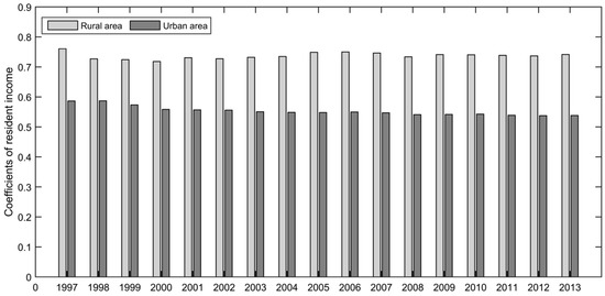
Figure 3.
Time varying-coefficients of resident income (α1t).
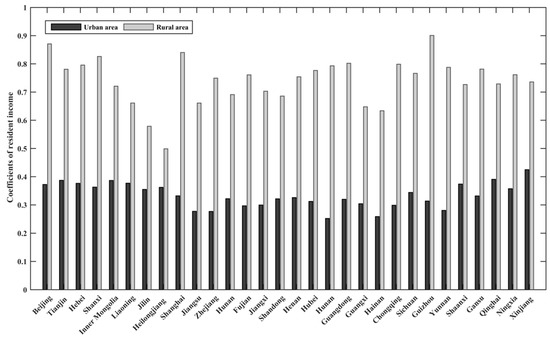
Figure 4.
Individual varying-coefficients of resident income across provinces (α1n).
R2 = 0.769; F = 55.772 (urban); R2 = 0.745 F = 45.119 (rural)
R2 = 0.612 F = 43.04 (urban) R2 = 0.334 F = 13.71 (rural)
In fact, the spatial heterogeneity between rural and urban households has more significant impact on the structure, pattern and efficiency of HEC than on the quantity of it [45,50,81,82]. First, the relatively perfect energy infrastructure, including central heating system, natural gas network system, power grids and filling stations, is build up in urban China. City dwellers easily access the high-quality energy, which is because dense population makes the relative cost of the construction down. Besides the electric grid, there are no other energy public infrastructures in the rural area. Thus, peasant families difficultly access natural gas and district heating, and drive longer distances to refuel motor vehicles. Coal accounts for almost 50% of total amount of commercial energy source consumed by them in 2013 (Figure 5), and they utilize some biomass fuels [48,72]. Second, if the various types of energy used by households are converted into effective heat, the “energy ladder” between rural and urban areas became clear [7,83]. By consuming the same amount of energy, an urban household uses the high-quality fuel, and obtains more effective heating than a rural household. Our previous study shows that per capita energy consumption in the provincial capital and rural area is 490.4 kgce and 456.1 kgce (including bio-fuels), respectively. Per capita effective heat is 323.3 kgce and 123.6 kgce, respectively [7]. However, the energy structure dominated by the fossil fuel is unfavorable to reduce GHG emissions.
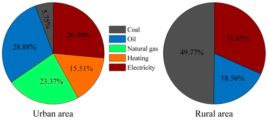
Figure 5.
The comparison of structure of energy consumption between urban resident and rural resident in China (2013).
5. Discussion and Conclusions
5.1. Discussion
Some studies adopted the data of total energy or total HEC in a region or country to analyze the relationship between urbanization and energy consumption [51,53,55,57]. It is inevitable to obtain results that urbanization promotes energy usage because the energy consumption necessarily increases with the growth of urban population. This is a mechanical effect of increase. To know whether urbanization improves the efficiency of energy-use, HEC per capita is used to discuss the issue. The result shows that the effect of urbanization on household energy use varies according to economic development stage. Urbanization decreases energy use in the western underdeveloped region, while its effect is mixed in the eastern region at middle-income level. Therefore, it is inadvisable to advocate that China should slow the process of urbanization to combat global climate change [57]. Instead, China should view urbanization as an opportunity to save energy and reduce emissions [53].
There is concern that the share of fossil fuel in HEC is increasing. With outflow of rural population and increasing use of modern fuel in rural households, there is more surplus biomass energy. Although biomass energy is non-commercial energy source, its use is still influenced by economic factors. In addition, the urban resident with relatively high income does not use biomass energy because its energy intensity is low and it discharges many pollutants caused by burning. Rural households usually cut-down on their usage of bio-fuel as their incomes increase. The comprehensive utilization of crop straw becomes a new problem in China. According to Sun’s estimation [28], actual amount of household energy consumption in rural areas of China is greater than data from Energy Statistical Yearbook (State Statistical Bureau, 1998–2014). If the source of household energy use in rural areas includes biomass fuel, the difference in per capita household energy consumption (kgce) between urban and rural area will become not significant. Other studies argued that total energy consumption in rural households exceeds that in urban households because of a continued dependence on inefficient solid fuels [37]. When explained variable in rural area increases in Equations (5) and (6), constants and income coefficients will also increase, which does not change the trend of the spatial heterogeneity in energy consumption between rural and urban households.
In existing scientific literature, temperature is regarded as a function of time. Thus, the temperature fluctuation in time series is used to examine its impact on HEC for the given region. The impact of temperature variations on energy consumption for heating and cooling is the most sensitive [10,11,32,34]. In this study, to reflect the regional differences, the temperature is regarded as the spatial function of energy consumption. The inter-annual temperature fluctuates up and down in a region, and value of the temperature variation in a region is far less than the value of temperature difference between regions. Thus, the spatial effect of temperature on HEC is more significant than the time effect of it. Our result shows the trend of the impact of temperature fluctuation on energy use in household sector.
The local spatial difference between urban and rural areas has more significant impact on the structure and efficiency of household energy consumption than on the quantity of it. In the rural areas, in order to enhance the availability of high-quality energy, energy public infrastructure should be improved. Thus, it is necessary to develop the new technology that solid biomass, such as crop straw, dung and firewood, are converted into biogas and liquid fuels. Then, clean energy can be used for heating and cooking for the rural resident [84]. In addition, the growth of clean energy should be accelerated to gradually change the structure of energy source dominated by fossil fuel at present [85]. There are rich renewable energy sources in western China, such as solar energy, wind power and hydropower. Meanwhile, Industrial surplus heat can be used for district heating in urban areas [86].
Based on the literature review in Section 2, we chose three key variables having larger impact on household energy consumption in macro-scale. Some factors, such as fuel price and demographic characteristic, lack significant spatial difference. Other factors, such as infrastructure conditions and resident’s lifestyles, lack full database at the provincial level. Besides, there is spatial difference in precipitation and wind speed, but they have little impact on HEC. As limitations of this study, we will investigate the impact of these factors on spatial difference of HEC in future work.
5.2. Conclusions
Household energy consumption is influenced by many factors. These factors exert influence on the amount, structure and pattern of energy use in various ways. Based on the STIRPAT model and panel dataset for 30 provinces in China over the period 1997–2013, effects of GDP per capita, urbanization level and annual average temperature on HEC per capita were investigated. The estimation results show that GDP per capita (lnGDP) has a significant positive impact on household energy consumption for 13 different models. A 1% increase in GDP per capita (thousand Yuan) would lead to 0.75% increase in energy consumption per capita (kgce) when other factors are invariable. It is the same result if resident income (IN) is substituted for GDP, and income contributions to energy use are positive in all models. This indicates that economic level is a key factor influencing household fuel consumption. It is also worth attention that there exists a diminishing marginal contribution with increasing income.
The elasticity coefficients of urbanization level (lnURB) are negative for most models, which indicate that a 1% increase in urbanization level would decrease household energy use per capita by around 0.54%. However, if lnGDP terms are taken out from all models, all values of elasticities of lnURB will become positive (Table 5), which means that there is a collinearity between lnGDP and lnURB, and these two variables interact closely. In addition, the impact of urbanization on HEC varies across the stages of economic development: it would decrease household energy use in the less developed western region, while it has mixed results in the relatively developed eastern region.
The effects of temperature on HEC are negative for all models, which express the opposite correlation between climatic conditions and energy consumption. The negative coefficients of lnTEM indicate that a 1% increase in annual average temperature would decrease energy consumption per capita by 0.12%–0.823%.
The spatial heterogeneity in HEC has multiscale behavior. At the provincial level, quantitative variation in the east–west direction largely depends upon economic development level, followed by the temperature. The elasticity coefficients of lnGDP in the western region are always greater than that in the eastern region, which indicates the effect of resident income on HEC in less developed region is more sensitive than that in the relatively developed region. The change in north–south direction is mainly determined by temperature. The intercept terms estimated by models in the most north provinces are positive, and those in the most southern provinces are negative, which indicates that the cardinal number of HEC is greater for heating in long and cold winter in north provinces. In addition, the results estimated by dummy variables for most models show that the difference between urban and rural areas in quantity of HEC is not significant, while those in the structure and efficiency are significant. This is because there is relatively good energy infrastructure in urban areas and the urban residents have higher incomes.
GDP or income per capita and urbanization level are increasing annually; they not only have the time effect on energy consumption but also the spatial effect, while annual average temperature is relatively stable on inter-annual timescale. These three factors affect energy consumption in household sector together, while showing their own spatial difference. These results are worth paying attention to for energy policy makers and planners in China.
To meet the global challenge of climate change and the need of China’s urbanization transformation, it is necessary to accelerate the development of renewable energy, and improve the rural energy infrastructure. In addition, to reduce emissions in China, we should focus on energy structure optimization and efficiency improvement, and build up the low-carbon oriented household energy system [87,88].
Acknowledgments
This work has been supported by the National Natural Science Foundation of China (Grant No. 41171437) and National Social Science Foundation of China (Grant No. 15CJY034). The authors wish to thank two anonymous reviewers for their constructive suggestions to improve the quality of this article.
Author Contributions
Yongxia Ding and Wei Qu reviewed the literature, analyzed results and wrote the majority of the manuscript. Shuwen Niu designed the research and drew conclusions. Wenli Qiang joined discussion. Man Liang and Zhenguo Hong collected the data and made figures. All authors have read and approved the final manuscript.
Conflicts of Interest
The authors declare no conflict of interest.
Nomenclature
| STIRPAT | Stochastic Impacts by Regression on Population, Affluence and Technology |
| CDD | cooling degree-days |
| HDD | heating degree days |
| GDP | per capita (Yuan) |
| IN | household income (Yuan) |
| URB | urbanization level (%) |
| TEM | annual average temperature (°C) |
| HEC | household energy consumption |
| Kgce | equivalent of coal (kg) |
| GHG | greenhouse gas |
Appendix A
Table A1.
Panel unit root tests.
| Variable | Levels | First Differences | ||||||
|---|---|---|---|---|---|---|---|---|
| LLC | IPS | ADF | PP | LLC | IPS | ADF | PP | |
| LnEnp | 6.338 | 12.429 | 4.437 | 5.730 | −3.325 *** | −3.852 *** | 98.916 *** | 108.537 *** |
| LnGDP | 10.050 | 17.186 | 18.660 | 12.988 | −5.147 *** | −2.753 *** | 82.537 ** | 64.115 |
| lnURB | −7.138 *** | 1.899 | 52.395 | 153.019 *** | −14.450 *** | −11.121 *** | 224.337 *** | 245.615 *** |
| lnTEM | −11.628 *** | −9.461 *** | 196.242 *** | 215.698 *** | −22.923 *** | −21.799 *** | 433.780 *** | 586.070 *** |
| LnEup | 4.447 | 8.725 | 10.098 | 9.765 | −12.789 *** | −11.587 *** | 232.969 *** | 254.766 *** |
| LnErp | 4.315 | 7.331 | 17.539 | 25.008 | −15.850 *** | −12.968 *** | 259.267 *** | 308.876 *** |
| lnINu | 11.853 | 18.665 | 0.357 | 0.334 | −8.417 *** | −7.098 *** | 150.354 *** | 164.475 *** |
| lnRINr | 5.310 | 11.361 | 2.694 | 2.514 | −22.241 *** | −22.506 *** | 434.598 *** | 364.338 *** |
** p < 0.05, *** p < 0.01.
Appendix B
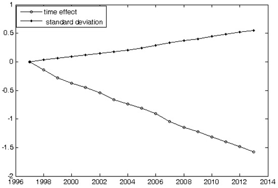
Figure B1.
The time effect of model FE-TW.
References
- Zhao, X.; Li, N.; Ma, C. Residential energy consumption in urban China: A decomposition analysis. Energy Policy 2012, 41, 644–653. [Google Scholar] [CrossRef]
- Yue, T.; Long, R.; Chen, H. Factors influencing energy-saving behavior of urban households in Jiangsu Province. Energy Policy 2013, 62, 665–675. [Google Scholar] [CrossRef]
- Wang, Z.; Zhang, B.; Yin, J.; Zhang, Y. Determinants and policy implications for household electricity-saving behaviour: Evidence from Beijing, China. Energy Policy 2011, 39, 3550–3557. [Google Scholar] [CrossRef]
- Chen, Q. The Sustainable Economic Growth, Urbanization and Environmental Protection in China. Available online: http://go.galegroup.com/ps/anonymous?id=GALE|A317588325&sid=googleScholar&v=2.1&it=r&linkaccess=fulltext&issn=1556763X&p=AONE&sw=w&authCount=1&isAnonymousEntry=true (accessed on 15 November 2016).
- Grimm, N.B.; Foster, D.; Groffman, P.; Grove, J.M.; Hopkinson, C.S.; Eadelhoffer, K.J.; Pataki, D.E.; Peters, D.P.C. The changing landscape: Ecosystem responses to urbanization and pollution across climatic and societal gradients. Front. Ecol. Environ. 2008, 6, 264–272. [Google Scholar] [CrossRef]
- Kahrl, F.; Roland-Holst, D. Growth and structural change in China’s energy economy. Energy 2009, 34, 894–903. [Google Scholar] [CrossRef]
- Niu, S.; Zhang, X.; Zhao, C.; Niu, Y. Variations in energy consumption and survival status between rural and urban households: A case study of the Western Loess Plateau, China. Energy Policy 2012, 49, 515–527. [Google Scholar] [CrossRef]
- Jorge, R.; Claudia, S.; David, M. The structure of household energy consumption and related CO2 emissions by income group in Mexico. Energy Sustain. Dev. 2010, 14, 127–133. [Google Scholar]
- Niu, S.; Jia, Y.; Ye, L.; Dai, R.; Li, N. Does electricity consumption improve residential living status in less developed regions? An empirical analysis using the quantile regression approach. Energy 2016, 95, 550–560. [Google Scholar] [CrossRef]
- Fikru, M.G.; Gautier, L. The impact of weather variation on energy consumption in residential houses. Appl. Energy 2015, 144, 19–30. [Google Scholar] [CrossRef]
- Considine, T.J. The impacts of weather variations on energy demand and carbon emissions. Resour. Energy Econ. 2000, 22, 295–314. [Google Scholar] [CrossRef]
- Alberini, A.; Filippini, M. Response of residential electricity demand to price: The effect of measurement error. Energy Econ. 2010, 33, 889–895. [Google Scholar] [CrossRef]
- Cole, M.A.; Neumayer, E. Examining the Impact of Demographic Factors on Air Pollution. Popul. Environ. 2004, 26, 5–21. [Google Scholar] [CrossRef]
- Wang, X.; Dai, X.; Zhou, Y. Domestic energy consumption in rural China: A study on Sheyang County of Jiangsu Province. Biomass Bioenergy 2002, 22, 251–256. [Google Scholar]
- Niu, S.; Zhang, X.; Zhao, C.; Ding, Y.; Niu, Y.; Christensen, T.H. Household energy use and emission reduction effects of energy conversion in Lanzhou city, China. Renew. Energy 2011, 36, 1431–1436. [Google Scholar] [CrossRef]
- Zhou, S.; Teng, F. Estimation of urban residential electricity demand in China using household survey data. Energy Policy 2013, 61, 394–402. [Google Scholar] [CrossRef]
- Chen, X.; Wen, Y.; Li, N. Energy Efficiency and Sustainability Evaluation of Space and Water Heating in Urban Residential Buildings of the Hot Summer and Cold Winter Zone in China. Sustainability 2016, 8, 989. [Google Scholar] [CrossRef]
- Zhang, M.; Guo, F. Analysis of rural residential commercial energy consumption in China. Energy 2013, 52, 222–229. [Google Scholar] [CrossRef]
- Ping, X.; Li, C.; Jiang, Z. Household energy consumption patterns in agricultural zone, pastoral zone and agro-pastoral transitional zone in eastern part of Qinghai-Tibet Plateau. Biomass Bioenergy 2013, 58, 1–9. [Google Scholar] [CrossRef]
- Lu, H.; Liu, G. Spatial effects of carbon dioxide emissions from residential energy consumption: A county-level study using enhanced nocturnal lighting. Appl. Energy 2014, 131, 297–306. [Google Scholar] [CrossRef]
- Zhang, L.; Yang, Z.; Liang, J.; Cai, Y. Spatial Variation and Distribution of Urban Energy Consumptions from Cities in China. Energies 2010, 4, 26–38. [Google Scholar] [CrossRef]
- Xu, S.C.; He, Z.X.; Long, R.Y.; He, Z.X. Factors that influence carbon emissions due to energy consumption in China: Decomposition analysis using LMDI. Appl. Energy 2014, 127, 182–193. [Google Scholar] [CrossRef]
- Jiang, L.; Ji, M.H. China’s Energy Intensity, Determinants and Spatial Effects. Sustainability 2016, 8, 544. [Google Scholar] [CrossRef]
- Wang, X.; Feng, Z. Common factors and major characteristics of household energy consumption in comparatively well-off rural China. Renew. Sustain. Energy Rev. 2003, 7, 545–552. [Google Scholar]
- Qi, Y.; Li, H.; Wu, T. Interpreting China’s carbon flows. Proc. Natl. Acad. Sci. USA 2013, 110, 11221–11222. [Google Scholar] [CrossRef] [PubMed]
- Niu, S.W.; Li, Y.X.; Ding, Y.X.; Qin, J. Energy demand for rural household heating to suitable levels in the Loess Hilly Region, Gansu Province, China. Energy 2010, 35, 2070–2078. [Google Scholar] [CrossRef]
- Delmastro, C.; Lavagno, E.; Mutani, G. Chinese residential energy demand: Scenarios to 2030 and policies implication. Energy Build. 2015, 89, 49–60. [Google Scholar] [CrossRef]
- Sun, J.W. Real rural residential energy consumption in China, 1990. Energy Policy 1996, 24, 827–839. [Google Scholar] [CrossRef]
- Henley, A.; Peirson, J. Non-Linearities in Electricity Demand and Temperature: Parametric Versus Non-Parametric Methods. Oxf. Bull. Econ. Stat. 1997, 59, 149–162. [Google Scholar] [CrossRef]
- Bessec, M.; Fouquau, J. The non-linear link between electricity consumption and temperature in Europe: A threshold panel approach. Energy Econ. 2008, 30, 2705–2721. [Google Scholar] [CrossRef]
- Ruth, M.; Lin, A.C. Regional energy demand and adaptations to climate change: Methodology and application to the state of Maryland, USA. Energy Policy 2006, 34, 2820–2833. [Google Scholar] [CrossRef]
- Mirasgedis, S.; Sarafidis, Y.; Georgopoulou, E.; Kotroni, V.; Lagouvardos, K.; Lalas, D.P. Modeling framework for estimating impacts of climate change on electricity demand at regional level: Case of Greece. Energy Convers. Manag. 2007, 48, 1737–1750. [Google Scholar] [CrossRef]
- Isaac, M.; Vuuren, D.P.V. Modeling global residential sector energy demand for heating and air conditioning in the context of climate change. Energy Policy 2009, 37, 507–521. [Google Scholar] [CrossRef]
- Kaufmann, R.K.; Gopal, S.; Tang, X.; Raciti, S.M.; Lyons, P.E.; Geron, N.; Craig, F. Revisiting the weather effect on energy consumption: Implications for the impact of climate change. Energy Policy 2013, 62, 1377–1384. [Google Scholar] [CrossRef]
- Parkpoom, S.J.; Harrison, G.P. Analyzing the Impact of Climate Change on Future Electricity Demand in Thailand. IEEE Trans. Power Syst. 2008, 23, 1441–1448. [Google Scholar] [CrossRef]
- Komatsu, S.; Ha, H.D.; Kaneko, S. The effects of internal migration on residential energy consumption and CO 2 emissions: A case study in Hanoi. Energy Sustain. Dev. 2013, 17, 572–580. [Google Scholar] [CrossRef]
- Pachauri, S.; Jiang, L. The household energy transition in India and China. Energy Policy 2008, 36, 4022–4035. [Google Scholar] [CrossRef]
- Li, K.; Lin, B. Impacts of urbanization and industrialization on energy consumption/CO2 emissions: Does the level of development matter? Renew. Sustain. Energy Rev. 2015, 52, 1107–1122. [Google Scholar] [CrossRef]
- Lee, C.C.; Chiu, Y.B. Electricity demand elasticities and temperature: Evidence from panel smooth transition regression with instrumental variable approach. Energy Econ. 2011, 33, 896–902. [Google Scholar] [CrossRef]
- Poumanyvong, P.; Kaneko, S. Does urbanization lead to less energy use and lower CO2 emissions? A cross-country analysis. Ecol. Econ. 2010, 70, 434–444. [Google Scholar] [CrossRef]
- Nie, H.; Kemp, R. Index decomposition analysis of residential energy consumption in China: 2002–2010. Appl. Energy 2014, 121, 10–19. [Google Scholar] [CrossRef]
- Liddle, B.; Lung, S. Age-structure, urbanization, and climate change in developed countries: Revisiting STIRPAT for disaggregated population and consumption-related environmental impacts. Popul. Environ. 2010, 31, 317–343. [Google Scholar] [CrossRef]
- York, R. Demographic trends and energy consumption in European Union Nations, 1960–2025. Soc. Sci. Res. 2007, 36, 855–872. [Google Scholar] [CrossRef]
- Kaza, N. Understanding the spectrum of residential energy consumption: A quantile regression approach. Energy Policy 2010, 38, 6574–6585. [Google Scholar] [CrossRef]
- Wei, Y.M.; Liu, L.C.; Fan, Y.; Wu, G. The impact of lifestyle on energy use and CO2 emission: An empirical analysis of China’s residents. Energy Policy 2007, 35, 247–257. [Google Scholar] [CrossRef]
- Ruijven, B.J.V.; Vuuren, D.P.V.; Vries, B.J.M.D.; Isaac, M.; Sluijs, J.P.V.D.; Lucas, P.L.; Balachandra, P. Model projections for household energy use in India. Energy Policy 2011, 39, 7747–7761. [Google Scholar] [CrossRef]
- Chen, S.; Li, N.; Yoshino, H.; Guan, J.; Levine, M.D. Statistical analyses on winter energy consumption characteristics of residential buildings in some cities of China. Energy Build. 2010, 43, 136–146. [Google Scholar] [CrossRef]
- Zheng, X.; Wei, C.; Qin, P.; Guo, J.; Yu, Y.; Song, F.; Chen, Z. Characteristics of residential energy consumption in China: Findings from a household survey. Energy Policy 2014, 75, 126–135. [Google Scholar] [CrossRef]
- Groh, S.; Pachauri, S.; Rao, N. What are we measuring? An empirical analysis of household electricity access metrics in rural Bangladesh. Energy Sustain. Dev. 2016, 30, 21–31. [Google Scholar] [CrossRef]
- Zhou, Y.; Liu, Y.; Wu, W.; Li, Y. Effects of rural–urban development transformation on energy consumption and CO2 emissions: A regional analysis in China. Renew. Sustain. Energy Rev. 2015, 52, 863–875. [Google Scholar] [CrossRef]
- Yuan, B.; Ren, S.; Chen, X. The effects of urbanization, consumption ratio and consumption structure on residential indirect CO2 emissions in China: A regional comparative analysis. Appl. Energy 2015, 140, 94–106. [Google Scholar] [CrossRef]
- Chikaraishi, M.; Fujiwara, A.; Kaneko, S.; Poumanyvong, P.; Komatsu, S.; Kalugin, A. The moderating effects of urbanization on carbon dioxide emissions: A latent class modeling approach. Technol. Forecast. Soc. Chang. 2015, 90, 302–317. [Google Scholar] [CrossRef]
- Wang, Q. Effects of urbanisation on energy consumption in China. Energy Policy 2014, 65, 332–339. [Google Scholar] [CrossRef]
- Wang, W.; Niu, S.; Jinghui, Q.I.; Ding, Y.; Na, L.I. The Correlation and Spatial Differences between Residential Energy Consumption and Income in China. Resour. Sci. 2014, 36, 1434–1441. (In Chinese) [Google Scholar]
- Sun, C.; Ouyang, X.; Cai, H.; Luo, Z.; Li, A. Household pathway selection of energy consumption during urbanization process in China. Energy Convers. Manag. 2014, 84, 295–304. [Google Scholar] [CrossRef]
- Poumanyvong, P.; Kaneko, S.; Dhakal, S. Impacts of urbanization on national transport and road energy use: Evidence from low, middle and high income countries. Energy Policy 2012, 46, 268–277. [Google Scholar] [CrossRef]
- Zhang, C.; Lin, Y. Panel estimation for urbanization, energy consumption and CO2 emissions: A regional analysis in China. Energy Policy 2012, 49, 488–498. [Google Scholar] [CrossRef]
- Dai, H.; Masui, T.; Matsuoka, Y.; Fujimori, S. The impacts of China’s household consumption expenditure patterns on energy demand and carbon emissions towards 2050. Energy Policy 2012, 50, 736–750. [Google Scholar] [CrossRef]
- Daioglou, V.; Ruijven, B.J.V.; Vuuren, D.P.V. Model projections for household energy use in developing countries. Energy 2012, 37, 601–615. [Google Scholar] [CrossRef]
- O’Neill, B.C.; Ren, X.; Jiang, L.; Dalton, M. The effect of urbanization on energy use in India and China in the iPETS model. Energy Econ. 2012, 34, S339–S345. [Google Scholar] [CrossRef]
- Liu, Y. Exploring the relationship between urbanization and energy consumption in China using ARDL (autoregressive distributed lag) and FDM (factor decomposition model). Energy 2009, 34, 1846–1854. [Google Scholar] [CrossRef]
- Druckman, A.; Jackson, T. Household energy consumption in the UK: A highly geographically and socio-economically disaggregated model. Energy Policy 2008, 36, 3177–3192. [Google Scholar] [CrossRef]
- Murata, A.; Kondou, Y.; Hailin, M.; Weisheng, Z. Electricity demand in the Chinese urban household-sector. Appl. Energy 2008, 85, 1113–1125. [Google Scholar] [CrossRef]
- Zachariadis, T.; Pashourtidou, N. An empirical analysis of electricity consumption in Cyprus. Energy Econ. 2007, 29, 183–198. [Google Scholar] [CrossRef]
- Halicioglu, F. Residential electricity demand dynamics in Turkey. Energy Econ. 2007, 29, 199–210. [Google Scholar] [CrossRef]
- Joyeux, R.; Ripple, R.D. Household energy consumption versus income and relative standard of living: A panel approach. Energy Policy 2007, 35, 50–60. [Google Scholar] [CrossRef]
- Liddle, B. Demographic Dynamics and Per Capita Environmental Impact: Using Panel Regressions and Household Decompositions to Examine Population and Transport. Popul. Environ. 2004, 26, 23–39. [Google Scholar] [CrossRef]
- Pachauri, S. An analysis of cross-sectional variations in total household energy requirements in India using micro survey data. Energy Policy 2004, 32, 1723–1735. [Google Scholar] [CrossRef]
- Holtedahl, P.; Joutz, F.L. Residential electricity demand in Taiwan. Energy Econ. 2004, 26, 201–224. [Google Scholar] [CrossRef]
- Tuan, N.A.; Lefevre, T. Analysis of household energy demand in Vietnam. Energy Policy 1996, 24, 1089–1099. [Google Scholar] [CrossRef]
- Parikh, J.; Shukla, V. Urbanization, energy use and greenhouse effects in economic development: Results from a cross-national study of developing countries. Glob. Environ. Chang. 1995, 5, 87–103. [Google Scholar] [CrossRef]
- Cai, J.; Jiang, Z. Changing of energy consumption patterns from rural households to urban households in China: An example from Shaanxi Province, China. Renew. Sustain. Energy Rev. 2008, 12, 1667–1680. [Google Scholar] [CrossRef]
- DeFries, R.; Pandey, D. Urbanization, the energy ladder and forest transitions in India’s emerging economy. Land Use Policy 2010, 27, 130–138. [Google Scholar] [CrossRef]
- Dietz, T.; Rosa, E.A. Rethinking the environmental impacts of population, Affluence and technology. Hum. Ecol. Rev. 1994, 1, 277–300. [Google Scholar]
- York, R.; Rosa, E.A.; Dietz, T. STIRPAT, IPAT and ImPACT: Analytic tools for unpacking the driving forces of environmental impacts. Ecol. Econ. 2003, 46, 351–365. [Google Scholar] [CrossRef]
- Hsiao, C. Analysis of Panel Data, 2nd ed.; Cambridge University Press: New York, NY, USA, 2003; pp. 1–10. [Google Scholar]
- National Bureau of Statistics of the People’s Republic of China. China Energy Statistical Yearbook; China Statistical Press: Beijing, China, 1998–2014.
- National Bureau of Statistics of the People’s Republic of China. China Statistical Yearbook; China Statistical Press: Beijing, China, 1998–2014.
- National Meteorological Information Center. Available online: http://data.cma.cn (accessed on 15 November 2016).
- Belloumi, M.; Alshehry, A.S. The Impact of Urbanization on Energy Intensity in Saudi Arabia. Sustainability 2016, 8, 375. [Google Scholar] [CrossRef]
- Joon, V.; Chandra, A.; Bhattacharya, M. Household energy consumption pattern and socio-cultural dimensions associated with it: A case study of rural Haryana, India. Biomass Bioenergy 2009, 33, 1509–1512. [Google Scholar] [CrossRef]
- Ekholm, T.; Krey, V.; Pachauri, S.; Riahi, K. Determinants of household energy consumption in India. Energy Policy 2010, 38, 5696–5707. [Google Scholar] [CrossRef]
- Ruijven, B.V.; Urban, F.; Benders, R.M.J.; Moll, H.C.; Sluijs, J.P.V.D. Modeling Energy and Development: An Evaluation of Models and Concepts. World Dev. 2008, 36, 2801–2821. [Google Scholar] [CrossRef]
- Nansaior, A.; Patanothai, A.; Rambo, A.T.; Simaraks, S. Climbing the energy ladder or diversifying energy sources? The continuing importance of household use of biomass energy in urbanizing communities in Northeast Thailand. Biomass Bioenergy 2011, 35, 4180–4188. [Google Scholar] [CrossRef]
- Park, E.; Han, T.; Kim, T.; Sang, J.K.; Pobil, A.P.D. Economic and Environmental Benefits of Optimized Hybrid Renewable Energy Generation Systems at Jeju National University, South Korea. Sustainability 2016, 8, 877. [Google Scholar] [CrossRef]
- Li, Y.; Xia, J.; Fang, H.; Su, Y.; Jiang, Y. Case study on industrial surplus heat of steel plants for district heating in Northern China. Energy 2016, 102, 397–405. [Google Scholar] [CrossRef]
- Tian, X.; Geng, Y.; Dai, H.; Fujita, T.; Wu, R.; Liu, Z.; Masui, T.; Yang, X. The effects of household consumption pattern on regional development: A case study of Shanghai. Energy 2016, 103, 49–60. [Google Scholar] [CrossRef]
- Zhang, N.; Wang, B. Toward a Sustainable Low-Carbon China: A Review of the Special Issue of “Energy Economics and Management”. Sustainability 2016, 8, 823. [Google Scholar] [CrossRef]
© 2016 by the authors; licensee MDPI, Basel, Switzerland. This article is an open access article distributed under the terms and conditions of the Creative Commons Attribution (CC-BY) license (http://creativecommons.org/licenses/by/4.0/).