The Economic Value of the National Meteorological Service in the Korean Household Sector: A Contingent Valuation Study

Abstract

The meteorological service (MS) in Korea is provided by the Korea Meteorological Administration (KMA), a governmental organization. This study attempts to measure the economic value of the national MS in the Korean household sector. Economic theory indicates that the economic value of a service is the area under the demand curve, which is the sum of the actual expenditure and the additional willingness to pay (WTP) for the service. The actual expenditure is well known, but the additional WTP is not. Thus, we assess the additional WTP for the national MS, conducting a contingent valuation survey of 1000 randomly selected households in Korea in 2014. We use a one-and-one-half-bound dichotomous choice question to derive the WTP responses and apply a spike model to deal with WTP responses of zero. The mean additional WTP per household is computed as KRW 860 (USD 0.75) per month and is statistically significant at the 1% level. Given that the monthly expenditure for the MS is KRW 1459 (USD 1.26) per household as of 2013, the economic value of the national MS is computed as KRW 2319 (USD 2.01) per household per month. Expanding the value to the national population gives us KRW 513.6 billion (USD 444.9 million) per year.

1. Introduction

The meteorological service (MS) plays an important role and has pervasive effects in various sector of human life. This is because most people’s activity sectors (economic, public, and private sectors) are actually and seriously affected by the weather and climate conditions. Moreover, any uncertainties about severe weather and climate can cause financial loss and social risks to individuals, companies, and governments. Thus, the public announcement of accurately predicted weather and climate conditions, that is, the MS, is quite important throughout our community, contributing to people’s life, the economy, and industries. For example, the National Oceanic and Atmospheric Administration (NOAA) reported that weather- and climate-susceptible industry sectors account for nearly 30% of the United States’ gross domestic product [1].

Some studies in the literature have dealt with the importance of the climate and weather for tourism demand. For example, Perkins and Debbage [2] mentioned that meteorological events have the potential to exert a vast impact on business operations and profitability in outdoor-oriented sectors. In the same way, some studies have reported that the weather is a significant part of travel decision making and overall tourist gratification [3,4,5]. Kozak et al. [6] described the climate as playing a major resource role in beach tourism. Martin [7] reported that the climate has a role as a facilitator, making tourism activities enjoyable. Hewer and Gough [8] explored and assessed zoo visitors’ responses to seasonal climatic anomalies. Scott and Lemieux [9] explained that the tourism demand is motivated by certain climate and weather information. In addition, the increase in human mortality associated with seasonal characteristics has been studied in relation to human diseases, since thermal or cold environmental conditions can have a deadly effect on the health of individuals [10]. There is no end to the ways in which the weather and climate affect our lives. In summary, the meteorological agencies of other nations have been trying continuously to provide a weather service.

The MS in Korea is provided freely by the Korea Meteorological Administration (KMA), a governmental organization. With the help of the MS, people can make informed decisions to protect their health, safety, and security in the face of changing weather and environmental conditions. Accurate and timely forecasts and warnings are also critical to the optimum functioning of the Korean economy, in which many industries, including agriculture, energy production, transportation, and forestry, are directly affected by the weather conditions. A considerable amount of money is required for the KMA to provide the public with the MS. Currently, it is covered by the national taxes, and some people doubt whether the economic value of the national MS is greater than the costs involved in its provision. Therefore, policy makers are demanding information on the economic value of the national MS supplied by the KMA.

The prime objective of this paper is to measure the economic value of the national MS in the household sector using a specific case study of Korea. The consumer behavior theory of micro-economics indicates that the economic value of a service is the area under the demand curve [11,12,13,14,15], which is the sum of the actual expenditure and the additional willingness to pay (WTP) for the service. The actual expenditure is well-known information, but the additional WTP is not. Thus, we try to assess the additional WTP for the national MS using the contingent valuation (CV) approach. In particular, we use the one-and-one-half-bounded (OOHB) dichotomous choice (DC) question format provided by Cooper et al. [16] to elicit the WTP responses. This is because the OOHB DC question format can enhance the statistical efficiency by decreasing the response bias. Furthermore, this study applies the spike model suggested by Kriström [17] to deal with the WTP data with observations of zero.

In short, we attempt to examine the economic value of the national MS in the Korean household sector. A household is a unit of life that includes co-housing and livelihoods. In other words, a household consists of one or more people who live in the same habitation and also share at meals or living accommodation, and may consist of a single family or some other grouping of people [18]. In this context, we elicit the public’s additional WTP for the national MS service by using the CV method. More specifically, a combination of the OOHB DC model and the spike model is applied. The remainder of the paper is made up of five sections. A short review of earlier related studies is provided in Section 2. The methodology adopted in this study is explained in Section 3. The WTP model employed in the study is addressed in Section 4. The empirical results are reported and discussed in Section 5, and the final section provides our conclusions.

2. A Short Review of Previous Related Studies

Some studies in the literature have measured the economic value of an MS. Most used a survey-based stated preference technique, the CV method. It is one of the most popular methods used by environmental and resource economists to value environmental and non-market goods. As shown in

Table 1. A summary of some previous studies dealing with the economic value of a meteorological service using the stated preference method.

Countries	Source	Objects to Be Valued	Methods a	Mean WTP Estimates
China	[24]	Meteorological information: haze management and prevention	CV	Total value: USD 11 billion
Canada	[23]	Multiple commercial sectors	CV	USD 1.20 (agriculture sectors: USD 2.17, public sectors: USD 0.60)
United States	[22]	Improved hurricane forecasts	CE	USD 13 per household per year
United States	[21]	Improvement in meteorological prediction	CV	USD 17.88 per household per year (9 states of the USA)
Italy	[20]	Meteorological information in agriculture	CV	USD 44 to 447 per sector per year
Switzerland	[19]	Improvement in avalanche prediction	CV	USD 42 to 46 per person (for a one-off payment)
United States	[11]	Meteorological information	CV	USD 109 per household per year (whole country)

^a CV and CE denote contingent valuation and choice experiment, respectively.

, many studies have examined consumers’ WTP for an MS by employing a stated preference approach, such as the CV and choice experiment methods. For example, Alberini et al. [19] used a CV method to understand the public’s valuation of an MS through skiers’ WTP for avalanche forecasting in Switzerland. The mean WTP for improved services ranged between USD 42 and UDS 46 per person (for a one-off payment). Predicatori et al. [20] examined the value of meteorological information in agriculture in Italy using the CV approach. They presented an expense range for an improvement of the meteorological information in specific agricultural sectors, and the WTP range was USD 44 to 447 per sector per year.

Lazo and Chestnut [11] and Lazo [21] investigated the data obtained from a survey of US households aimed at measuring their preferences for current-level and improved weather forecasts and found a positive WTP. The economic values of the current-level and the improved weather forecasts in the USA were about USD 109 and USD 17.88 per household per year, respectively. Moreover, Lazo and Waldman [22] estimated the economic value of improved hurricane forecasts from a pilot CV survey and discovered that the mean WTP for the improved services was USD 13 per household per year. Rollins and Shaykewich [23] assessed the economic value of weather forecasts for multiple commercial sectors in Canada as USD 1.20 per use count (meteorological information by phone). Wang et al. [24] analyzed the public’s WTP for haze management and prevention using the CV method. Overall, the literature has shown that people reveal themselves to be willing to shoulder the burden of an additional cost for an MS. Of the above-mentioned seven case studies presented in Table 1, six studies used CV. Thus, the strategy of employing CV in our study is consistent with the practices of former studies.

3. Methodology

3.1. Object to Be Valued

The object to be valued in this study is the national MS provided by the KMA of Korea. The KMA provides the public with weather forecasts through multiple media channels, including broadcasting networks, newspapers, and the Internet, reporting the expected humidity, state of the sky, snow cover, thunder and lighting, precipitation, probability of precipitation, Asian Dust, fog, temperature, wind direction, wind speed, and wave height. Moreover, the KMA supplies region-specific weather information services as well as hazardous meteorological information with regard to typhoons, tsunami, earthquakes, wind waves, and so on. The national MS uses a customized short message service providing the ultraviolet index, food poisoning index, and discomfort index, as well as a special weather report on heat waves and Asian Dust.

The household sector benefits from the national MS in four aspects [25]. First, the national MS can reduce many inconveniences caused by the situation without it. For example, we can prepare warm clothing if cold or snow is forecast, and we can prepare an umbrella if rain is predicted. Second, it can protect household members’ health. For instance, with its help, one can decrease the possibility of catching a cold or fever. Third, it can secure the safety of household. Forecasting heavy rainfall, heavy snowfall, or strong wind can significantly mitigate the risk of injury or death. Fourth, it can abate unnecessary expenditures which unexpected weather conditions demand of households. These were clearly conveyed to the respondents in the CV survey.

3.2. Method for Measuring the Economic Value of the MS: The CV Approach

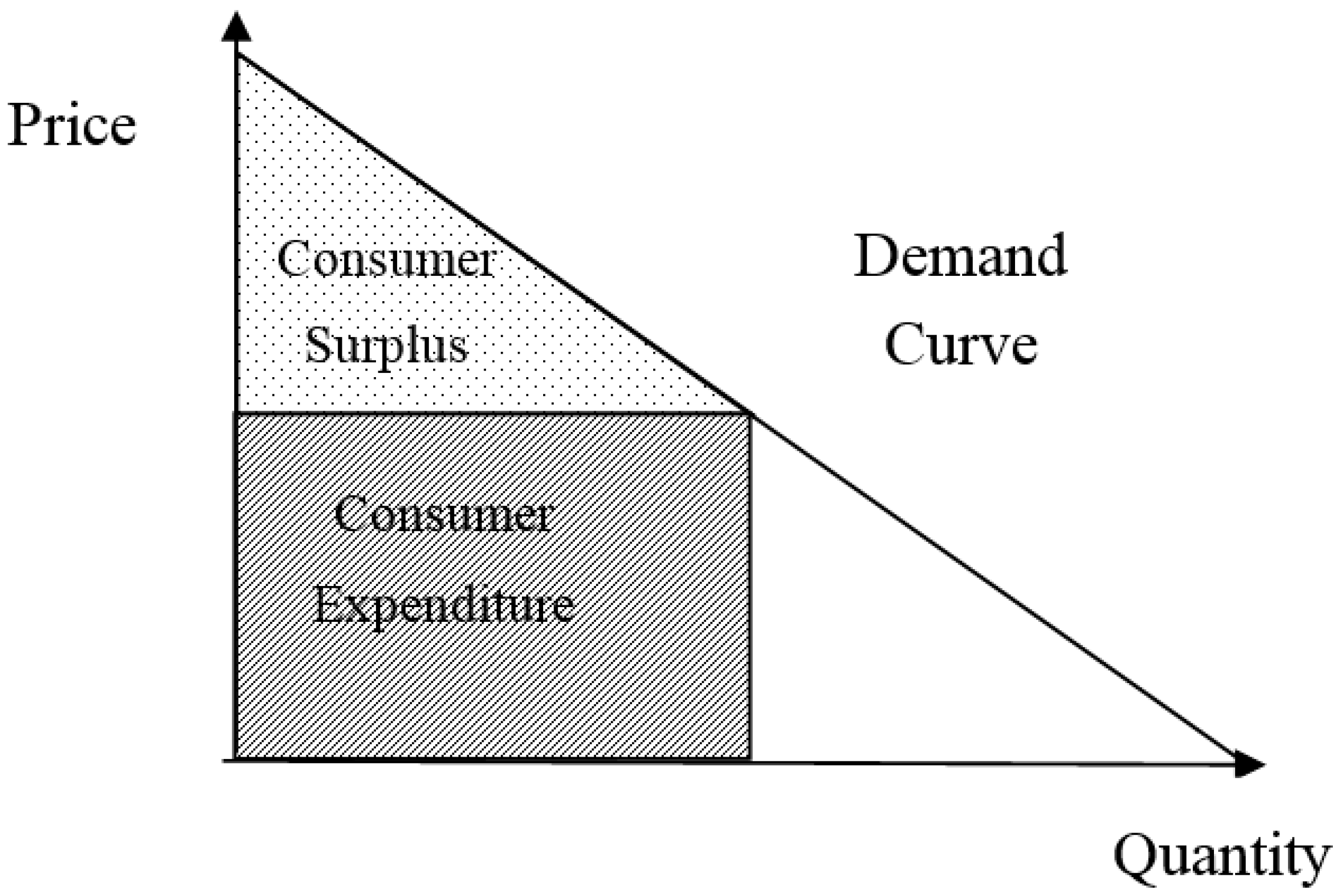
In the context of economics, the economic values of a service are defined as the area below the demand curve for the service. The area is precisely the consumers’ WTP for the service, and it is the sum of consumer surplus (CS) and actual payment [26]. The actual payment is expenditure to purchase and CS means the additional WTP. The CS is defined as the gap between a consumer’s additional WTP and the actual price, as shown in Figure 1. In other words, the economic benefits of the MS are the sum of the additional WTP and actual consumer expenditure. Thus, we can usually value the economic benefits by first estimating the demand function and then computing the area.

A rational consumer maximizes his/her utility under income or budget constraints. The demand for a good or service is derived as a solution to the utility maximization problem when the market exists and the price is exogenously given. It is natural that if the price changes the demand should also change. Thus, we can define the demand function where the price is an independent variable and the demand is a dependent variable. The demand function is assumed to be smooth and continuous. Given that the demand function exists and we can obtain it, microeconomic theory shows that we can utilize the demand function to assess the economic value of the MS [27,28].

However, if the service is not traded in the market, in other words it is a non-market good, estimating the demand function is quite difficult. The economic value of the national MS is a case for which directly calculating the area under the demand function is an appropriate strategy; this can be achieved using a stated preference technique such as the CV method.

The CV technique has been very widely applied in the literature to obtain the WTP for non-market goods. There are no restrictions on the objects that can be valued using the CV method. In particular, it is more useful than other methods because it can capture the non-use or existence value of a good that cannot be measured through a market mechanism. Non-market goods include environmental goods or public goods such as the national MS. Thus, as explained earlier, this study seeks to utilize the CV approach to assess the economic value of the national MS. It asks a potential consumer a question concerning the additional WTP for consistently receiving the national MS using a well-structured survey of randomly chosen consumers [29].

Some people may doubt the practicality and usefulness of the CV method because it gathers information from a survey of respondents. In this regard, the blue-ribbon NOAA Panel reached the influential conclusion that the CV method can produce reliable quantitative information that can be utilized in decision making both for public administrations and judicially, provided that several guidelines proposed by the NOAA Panel are observed [30]. Moreover, following the guidelines can secure the validity and accuracy of the CV method.

For example, the service of concern should be familiar to the public, the CV survey should be administered through face-to-face interviews by professionally trained interviewers rather than through telephone or mail interviews, a suitable payment vehicle should be adopted and presented to the respondents, and the substitutes for the goods should be explained to the respondents in the survey. These conditions were met in our study, as will be discussed in detail below.

3.3. Sampling and Survey Methods

We commissioned a professional survey firm to arrange the CV field survey. The firm drew a stratified random sample of 1000 households from the national population to obtain information on their additional WTP for the national MS and their socioeconomic characteristics. The survey firm (Research Prime Corporation, Seoul, Korea) is located on Seoul, the capital of Korea, and has a number of experiences of conducting a CV survey since 2003. A supervisor affiliated with the firm hired fifty well-trained interviewers across the nation and educated them. A CV survey can be conducted during face-to-face in-person, telephone, or mail interviews. The response rate to a mail survey is usually quite low, and a telephone survey can present only a limited volume of information to the respondents. In the CV survey, we wished to convey to the respondents a large amount of explanatory information on the national MS, to provide visual cards describing the situation with and without the national MS, and to outline the effects of the national MS. This is why we undertook face-to-face interviews.

We gave the interviewers sufficient information about the purposes and background of the CV survey and instructed them on how to answer the questions that might be raised by the interviewees in the CV survey. Moreover, the supervisors affiliated with the survey company trained the interviewers in implementing the CV survey as persuasively and effectively as possible. To derive reliable and responsible decision making from the respondents, 20- to 65-year-old heads of households or homemakers were selected and interviewed for the CV survey. Judging from the interviewers’ comments, the respondents gave their WTP responses without great difficulty. The survey was conducted in November 2014, and the final number of observations to be analyzed in our study was 1000.

The survey instrument consists of three parts. The first is an introductory section, explaining the general background information about the national MS and then asking the respondents about their perceptions of it. The scenario in which the goods to be valued would be provided to the public should be clearly explained. The second part includes questions about the respondents’ additional WTP for consistently receiving the national MS. These questions should be presented in a context that ensures that the additional WTP questions are plausible, understandable, and meaningful. The final part contains questions relating to the households’ socioeconomic variables.

3.4. Method of WTP Elicitation

Our study used a DC question format, which is a type of closed question. This is preferred in the literature to open-ended questions, because a respondent is likely to show strategic behavior and have difficulty in giving a WTP response when an open-ended question is asked. In addition, the blue-ribbon panel’s report [30] supported the use of a DC question rather than an open-ended question. In particular, the single-bounded (SB) DC question or double-bounded (DB) DC question is usually used. The SB DC question is a single DC question. By contrast, the DB DC question employs two DC questions. A respondent who answers “yes” to the first bid is additionally asked a follow-up question of whether he would pay a second, higher, bid. A respondent who answers “no” to the first bid is additionally asked a follow-up question concerning whether he would pay a second, lower bid.

The DB DC question format can significantly increase the statistical efficiency compared with the SB DC question format [31]. However, the DB DC question format also augments the response bias when compared with the SB DC question format [32,33,34]. Thus, SB DC and DB DC questions suffer from low statistical efficiency and high response bias, respectively. As an alternative to them, Cooper et al. [16] suggested the OOHB DC question format. The statistical efficiency of the OOHB DC question format is similar to that of the DB DC question format, and the consistency of the OOHB DC question format is close to that of the SB DC question format.

The OOHB DC question format is based on a set of two bids. In an OOHB DC question, the interviewer randomly selects one of two bids, which is then given to the respondent. If the selected bid is the lower one and the respondent’s response is “yes”, the remaining higher bid is presented to the respondent. If the selected bid is the lower one and the respondent’s response is “no”, a follow-up question is not needed. If the selected bid is the higher one and the respondent’s response is “yes”, a follow-up question is not necessary. If the selected bid is the higher one and the respondent’s response is “no”, the residual lower bid is then presented to the respondent.

We used seven sets of two bids, which were determined from a pretest on a focus group (30 persons). The list of the sets used in this study is as follows: (1000; 3000), (2000; 4000), (3000; 6000), (4000; 8000), (6000; 10,000), (8000; 12,000), and (10,000; 15,000). The numbers are in Korean won: the first element of each set is the lower bid and the second element is the higher bid. At the time of the survey, USD 1.0 was approximately equal to KRW 1155.

3.5. Payment Vehicle

Respondents may be embarrassed when asked directly for their additional WTP for the MS. Introducing into the survey questionnaire a medium through which the amount would be paid helps the respondents to reveal their true WTP. We usually call the medium the payment vehicle. The payment vehicles found in the literature include taxes, funds, donations, and expenditure. The respondents should feel at home with the payment vehicle, and the goods to be valued should have a clear connection with it. For this reason, a tax is most frequently employed in ascertaining the economic value of the provision of a public policy. There are two options: national and local taxes. Of the two, national tax is related to the national MS. Furthermore, among the several types of national tax, income tax is most familiar to the respondents [35,36]. Therefore, income tax is employed in this study as the payment vehicle.

Moreover, some additional statements concerning the payment were provided in the survey questionnaire. For example, the respondents were told: “You can see that your household paid a monthly service charge of KRW 1459 (USD 1.26) for the national MS. Would your household be willing to pay additional money in your service charge provided that the stable supply of the national MS is assured? The amount you indicate will tell us what it is really worth to your household to have access to the national MS”.

4. Modeling of WTP Responses

4.1. Basic WTP Model

There are two approaches to modeling WTP responses gathered from a DC CV survey: the utility difference approach suggested by Hanemann [37] and the WTP function approach proposed by Cameron and James [38]. The first specifies the utility difference using a random utility maximization model, while the second specifies the WTP responses directly. As pointed out by McConnell [39], the choice of one of these two is not an issue of right or wrong but rather depends on the researcher’s preference, because the two approaches are equivalent in the context of economics. The literature shows that the first has been more frequently applied than the second. Thus, we adopt the utility difference approach in our study. The ratios of “yes” responses to each given bid are the basic input when applying this approach.

Through the process of utility maximization under income constraint, a discrete choice response to the question of whether to pay a specified amount for achieving a given environmental improvement or the provision of a public good is derived for each respondent. The independent variables of the utility function, U, include the respondent’s income, socioeconomic characteristics, and perceptions about the good to be valued and its provision state. The provision state of the goods to be valued is S. The value of S is one if the good is provided and zero otherwise. The respondent’s income and the other factors that affect the respondent’s utility are $M$ and $T$. Thus, the utility function is defined as:

$$U=V(S,M;T)+\omega$$

(1)

where $V$ is the indirect utility function that we can obtain by inserting the solution to the utility maximization problem into the objective function of the respondent’s utility, $\omega$ is a random component of the utility, and the $\omega$ s are independent and identically distributed random variables with zero means.

The respondent will maximize her/his utility by showing that she/he is willing to pay a presented bid, $B$, to obtain the goods to be valued if:

$$V(1,M-B;T)+{\omega }_1\ge V(0,M;T)+{\omega }_0$$

(2)

Rearranging Equation (2) produces:

$$V(1,M-B;T)-V(0,M;T)\ge {\omega }_0-{\omega }_1$$

(3)

The left-hand side of Equation (3) is the utility difference, defined as $\Delta V$, and is the systematic and deterministic part, while the right-hand side is the non-systematic and random part. Let ${\omega }_0-{\omega }_1$ be $\theta$ and $H_{\theta }(\cdot )$ be the cumulative distribution function (cdf) of $\theta$. Using Equation (3), we can express the probability of obtaining the answer “yes” to a given bid as:

$$\mathrm{Pr}\{responseis“yes”\}=\mathrm{Pr}\{\Delta V(B)\ge \theta \}=H_{\theta }[\Delta V(B)]$$

(4)

From a different perspective, we can introduce the WTP, $X$, as a random variable in the description of the probability of reporting “yes” to a presented bid as follows.

$$\mathrm{Pr}\{responseis“yes”\}=\mathrm{Pr}\{X\ge B\}\equiv 1-F_X(B)$$

(5)

where $F_X(\cdot )$ is the cdf of $X$. Thus, comparing Equations (4) and (5) yields:

$$1-F_X(B)=H_{\theta }[\Delta V(B)]$$

(6)

Therefore, there is no need to assume the functional form of $H_{\theta }(\cdot )$; all that is necessary is to assume the functional form of $F_X(\cdot )$ and estimate its parameters. Usually, we assume that $\Delta V=\alpha -\beta B$, where $\lambda =(\alpha ,\beta )$, is a parameter vector to be estimated.

4.2. Model for Dealing with Zero WTP Responses: SPIKE Model

Some people can have an interest in the goods to be valued, but others may be totally indifferent to or place no value on the goods. In this case the proportion of zero WTP responses in the CV survey may be high. Researchers should pay close attention to how they deal with observations of WTP responses of zero. For this purpose we apply the spike model suggested by Kriström [17] and Yoo and Kwak [40]. The spike model specifies the probability of zero WTP responses as a spike at zero in the distribution of the WTP.

The spike model enables us to analyze both zero point and positive interval WTP data in a univariate setting. In the spike model, $F_X(B;\lambda )$ has the following functional form:

$$F_X(B;\lambda )=\{\begin{array}{l}{[1+\exp (\alpha -\beta B)]}^{-1}\mathrm{if}B>0\\ {[1+\exp (\alpha )]}^{-1}\mathrm{if}B=0\\ 0\mathrm{if}B<0\end{array}$$

(7)

As explained earlier, the spike is defined as the probability of the respondent’s WTP being zero. Thus, the spike is computed as ${[1+\exp (\alpha )]}^{-1}$. Some covariates, such as the respondent’s household income, can be incorporated into the spike model. A common method makes the covariates penetrate $\alpha$ in Equation (7). That is, $\alpha$ is simply changed to $\alpha +z^{\prime }\delta$, where $z$ is a vector of covariates and $\delta$ is a vector of the corresponding parameters to be estimated.

4.3. OOHB DC Model

As explained above, the OOHB DC model produces a higher level of statistical efficiency than the SB DC model and yields greater consistency than the DB DC model. This is why we use an OOHB DC model in this study instead of an SB or DB DC model. The following OOHB DC model is based on Cooper et al.’s [16] suggestion. We have $J$ observations to be analyzed. A bid, $B_j$, is given to respondent $j$ for $j=1,\mathrm{...},J$. During the CV survey, two bids, $B_j^L$ and $B_j^U$, where $B_j^L<B_j^U$, are presented to each respondent $j$.

About half of the respondents are provided with $B_j^L$ as the first bid. $B_j^U$ is supplied as the second bid if the answer is “yes”. In this case there are two outcomes, “yes–yes” ($X>B_j^U$) and “yes–no” ($B_j^L<X<B_j^U$). If the respondent answers “no” to the first bid, $B_j^L$, the outcome is “no” ($X<B_j^L$). The remaining respondents are presented with $B_j^U$ as the first bid. If the answer is “no”, the second bid, $B_j^L$, is sequentially supplied to the respondent and the possible outcomes are “no–yes” ($B_j^L<X<B_j^U$) and “no–no” ($X<B_j^L$). If the respondent’s response is “yes” ($X>B_j^U$), no further bid is required. Therefore, for the six results, we can introduce six binary variables, $I_j^{YY}$, $I_j^{YN}$, $I_j^N$, $I_j^{NY}$, $I_j^{NN}$, and $I_j^Y$. The value of each binary variable is one if the respondent’s response corresponds with its superscript and zero otherwise. For example, $I_j^{YY}$ is one if respondent $j$ reports “yes–yes” and zero otherwise.

4.4. OOHB DC Spike Model

In this subsection we attempt to combine the OOHB DC CV model and the spike model. To identify zero WTP observations, we asked the respondents who gave a “no” response when the first presented bid was $B_j^L$ or a “no–no” response when the first presented bid was $B_j^U$ an additional follow-up question that can distinguish true zero WTP from positive WTP. Thus, we can formulate one more binary variable, $I_j^P$, the value of which is one if the $j$ th respondent’s WTP is positive and zero otherwise. The log-likelihood function of the OOHB DC spike model is:

$$\begin{array}{l}\ln L={\displaystyle \sum _{j=1}^J\{(I_j^{YY}}+I_j^Y)\ln [1-F_X(B_j^U;\lambda )]\\ +(I_j^{YN}+I_j^{NY})\ln [F_X(B_j^U;\lambda )-F_X(B_j^L;\lambda )]\\ +I_j^P(I_j^N+I_j^{NN})\ln F_X(B_j^L;\lambda )\\ +(1-I_j^P)(I_j^N+I_j^{NN})\ln F_X(0;\lambda )\}\end{array}$$

(8)

Using Equation (7), the mean of the WTP can be computed as:

$$E(X)={\displaystyle {\int }_0^{\infty }[1-F_X(B;\alpha ,\beta )]dB-{\displaystyle {\int }_{-\infty }^0{F}_X(B;\alpha ,\beta )dB}}=\frac{1}{\beta }\ln {[1+\exp (\alpha )]}^{-1}$$

(9)

5. Results and Discussion

5.1. Data

The CV survey was administered to about 1400 randomly chosen households from the whole population of Korea during November 2014. Some observations that did not contain important information or were judged by the interviewers to be of poor quality were deleted from the final data set to be investigated. In this way we obtained 1000 useable observations.

Table 2. Distribution of the responses by each bid amount.

Bid Amount		Lower Bid Is Presented as the First Bid (%)				Upper Bid Is Presented as the First Bid (%)				Sample Size
Lower Bid	Upper Bid	Yes–Yes	Yes–No	No–Yes	No–No	Yes	No–Yes	No–No–Yes	No–No–No
1000	3000	7	18	7	40	4	12	13	42	143
		(4.9)	(12.6)	(4.9)	(28.0)	(2.8)	(8.4)	(9.1)	(29.4)	(100)
2000	4000	1	13	10	47	3	8	14	47	143
		(0.7)	(9.1)	(7.0)	(32.9)	(2.1)	(5.6)	(9.8)	(32.9)	(100)
3000	6000	1	8	19	51	2	6	17	47	143
		(0.7)	(5.6)	(13.3)	(35.7)	(1.4)	(4.2)	(11.9)	(32.9)	(100)
4000	8000	0	6	14	53	2	2	15	52	143
		(0.0)	(4.2)	(9.8)	(37.1)	(1.4)	(1.4)	(10.5)	(36.4)	(100)
6000	10,000	0	0	18	59	1	3	14	53	142
		(0.0)	(0.0)	(12.7)	(41.5)	(0.7)	(2.1)	(9.9)	(37.3)	(100)
8000	12,000	0	4	16	50	1	0	20	50	142
		(0.0)	(2.8)	(11.3)	(35.2)	(0.7)	(0.0)	(14.1)	(35.2)	(100)
10,000	15,000	0	2	13	52	1	3	15	53	144
		(0.0)	(1.4)	(9.0)	(36.1)	(0.7)	(2.1)	(10.4)	(36.8)	(100)
Totals		9	51	88	352	14	34	108	344	1000
		(0.9)	(5.1)	(8.8)	(35.2)	(1.4)	(3.4)	(10.8)	(34.4)	(100)

describes the distribution of responses by bid amount. Each set of bids was allocated to a similar number of respondents, as is shown in the last column of Table 2.

Both “no–no” responses when the lower bid was presented as the first bid and “no–no–no” responses when the upper bid was presented as the first bid indicate the zero WTP responses. A total of 696 households (69.6%) revealed zero additional WTP for the MS. This implies that the use of the spike model to deal with WTP responses of zero was a suitable approach in our study. Moreover, the zero WTP response is consistent with the microeconomic theory that non-consumption can be obtained as a corner solution to a utility maximization problem under income constraint. Overall, the proportion of “yes” responses to a given bid declines as the magnitude of the bid increases. For instance, when the lower bid was presented as the first bid, that is, when the bids moved “from lower bid to upper bid”, twenty-five respondents (17.5%) consented to pay KRW 1000 (USD 0.88), while just two respondents (1.4%) agreed to a payment of KRW 10,000 (USD 8.79).

5.2. Estimation Results of the OOHB DC Spike Model

The estimation results of the OOHB DC spike model are reported in

Table 3. Estimation results of the spike model.

Variables	Estimates d
Constant	−0.837 (−12.14) **
Bid a	−0.418 (−18.19) **
Spike	0.696 (47.99) **
Mean WTP per household per year	KRW 860 (USD 0.75)
t-value	13.47 **
95% confidence interval b	KRW 748 to 1000 (USD 0.65 to 0.87)
99% confidence interval b	KRW 717 to 1045 (USD 0.62 to 0.91)
Number of observations	1000
Log-likelihood	−857.60
Wald statistic (p-value) c	181.31 (0.000)

^a The unit is 1000 Korean won, and USD 1.0 was approximately equal to KRW 1155 at the time of the survey; ^b the confidence intervals are calculated by the use of the Monte Carlo simulation technique of Krinsky and Robb [41] with 5000 replications; ^c the null hypothesis is that all the parameters are jointly zero and the corresponding p-value is reported in the parentheses beside the statistic; ^d the numbers in parentheses beside the coefficient estimates are t-values, computed from the analytic second derivatives of the log-likelihood; the symbol ** indicates statistical significance at the 1% level.

. The parameter estimates can be obtained by finding the parameter values maximizing Equation (8), in other words, applying the maximum likelihood estimation method. All the estimates for the two parameters, $\alpha$ and $\beta$, are statistically significant at the 1% level. Moreover, the null hypothesis that the parameter estimates are all zero can be rejected at the 1% level, as the p-value for the Wald statistic calculated under the null hypothesis is less than 0.01. In particular, the estimate for the spike is 0.696, which coincides perfectly with the proportion of zero WTP responses in the sample provided in Table 3. This indicates that the spike model employed here fits our data well.

Using Equation (9) and the values presented in Table 3, we can obtain an estimate of the mean additional WTP of KRW 860 (USD 0.75) per household per month. Its t-value is 13.47; thus, the estimate is statistically meaningful at the 1% level. To handle the uncertainty related to the computation of the estimate, we try to report the confidence intervals for the estimate. For this purpose, the parametric bootstrapping method proposed by Krinsky and Robb [41] is the most widely employed in the literature. We use the method with 5000 replications to obtain the 95% and 99% confidence intervals, which are contained in Table 3. The 95% confidence interval is tighter than the 99% confidence interval.

5.3. Estimation Results of the OOHB DC Spike Model with Covariates

We seek to estimate the spike model with covariates explained in Section 4.2. Some variables used for the covariates are defined in

Table 4. Definitions and sample statistics of the variables.

Variables	Definitions	Mean	Standard Deviation
Education	The respondent’s education level in years	13.72	2.35
Gender	The respondent’s gender (1 = male; 0 = female)	0.50	0.50
Age	The respondent’s age in years	46.07	9.47
Income	The respondent’s household’s monthly income before tax deduction (unit: million Korean won = USD 865.8)	4.09	1.93

. They are related to the characteristics of the respondent or the respondent’s household. Furthermore, the sample statistics of the covariates are reported in Table 4. A total of four variables are contained in the model. The characteristics of the sample appear to reflect those of the population well, since we drew a random sample of Korean households with the help of the professional polling firm. The results of the spike model, including the variables shown in Table 4, are described in

Table 5. Estimation results of the spike model with covariates.

Variables a	Estimates	t-Values
Constant	−1.870	−2.89 **
Education	0.069	2.11 *
Gender	0.072	0.50
Age	−0.011	−1.41
Income	0.132	3.95 **
Bid amount b	−0.425	−17.81 **
Number of observations	1000
Log-likelihood	−842.08
Wald statistic c (p-value)	170.59 (0.000)

^a The variables are defined in Table 4; ^b the unit is 1000 Korean won, and USD 1.0 was approximately equal to KRW 1155 at the time of the survey; ^c the null hypothesis is that all the parameters are jointly zero, and the corresponding p-value is reported in the parentheses beside the statistic; the symbols ** and * indicate statistical significance at the 1% and the 5% level, respectively.

.

In particular, the coefficient estimates for Education and Income in the model are statistically significant at the 5% and the 1% level. The positive sign of the coefficient implies that the higher the value of the variable, the higher the likelihood of stating “yes” to a given bid. Thus, the respondent’s education level exerts a positive effect on the likelihood of voting “yes” to a given bid. The respondents with a higher income have a tendency to respond “yes” to the provided bid.

5.4. Discussion of the Results

As described earlier, the economic value of the MS in the household is calculated by summing the household’s current expenditure on the MS and the household’s additional WTP for the MS. As shown in Table 3, the mean additional WTP per household is computed as KRW 860 (USD 0.75) per month, given that the monthly expenditure for the MS is KRW 1459 (USD 1.26) per household as of 2013. Thus, the economic value of the national MS is computed as KRW 2319 (USD 2.01) per household per month.

To obtain an estimate of the total economic value, we need to use the mean WTP estimate obtained from the investigation of the sample observations and the information on population size. In the course of this estimation, the most important issue is whether or not the sample is representative of the population. As addressed above, the sampling was conducted by a professional survey firm to ensure its randomness and its consistency with the characteristics of the population. Another important issue is the response rate in the CV survey. Our CV survey was implemented using in-person face-to-face interviewing and thus the response rate was almost 100%. Therefore, we cannot deny that our sample is representative of the population.

We use the additional mean WTP estimate from the model with no covariates, since the setting of the covariates may influence the additional mean WTP value if we use the additional mean WTP value from the model with covariates. According to the Korean Statistical Information Service [42], the number of households in Korea was 18,457,628 at the time of the survey, November 2014. Using this information, expanding the value to the national population gives us KRW 513.6 billion (USD 444.9 million) per year, which is shown in

Table 6. Annual economic value of the national meteorological service (MS) in Korea.

Monthly Expenditure on the National MS	Monthly Additional Mean Willingness to Pay	Monthly Economic Value of the National MS	Annual Economic Value of the National MS
KRW 1459 (USD 1.26) per household	KRW 860 (USD 0.75) per household	KRW 2319 (USD 2.01) per household	KRW 513.6 billion (USD 444.9 million)

.

6. Conclusions

The national MS in Korea is provided by the KMA, a central governmental organization. Policy makers need quantitative information on the economic value of the national MS. Economic theory indicates that the economic value of a service is the area under the demand curve, which is the sum of the actual expenditure and the additional WTP for the service. The actual expenditure is well-known information, but the additional WTP is not. Thus, we attempted to assess the additional WTP for the MS, which is not known in Korea, by applying the CV approach. More specifically, we used an OOHB DC question to reduce any response bias involved in eliciting the WTP responses and employed the spike model to analyze the WTP responses with a number of zero observations.

The enumerators’ comments imply that the CV survey was successful in eliciting the additional WTP values from the respondents. The combination of the OOHB DC question and the spike model fit our data well, since all the parameter estimates of the spike model with no covariates are statistically meaningful at the 1% level. We found that the monthly mean additional WTP estimate from the OOHB DC spike model was KRW 860 (USD 0.75) per household. This value is statistically significant at the 1% level. Given that the expenditure on the current weather forecast services was KRW 1459 (USD 1.26) per household per month, the economic value of the current MS was estimated as KRW 2319 (USD 2.01) per household per month. Expanding the value to the national population gives us KRW 513.6 billion (USD 444.9 million) per year. It is clear from the results that the economic value of the national MS outweighs the costs related to it. That is, Korean households place a high value on the national MS.