Temporal Effects of Environmental Characteristics on Urban Air Temperature: The Influence of the Sky View Factor

Abstract

This study examines the relationship between air temperature and urban environment indices, mainly focusing on sky view factor (SVF) in Seoul, Korea. We use air temperature data observed from 295 automatic weather stations (AWS) during the day and night in Seoul. We conduct a spatial regression analysis to capture the effect of spatial autocorrelation in our data and identify changes in the effects of SVF on air temperature, while conducting the regression model for each dataset according to the floor area ratio (FAR). The findings of our study indicate that SVF negatively affects air temperature during both day and night when other effects are controlled through spatial regression models. Moreover, we address the environmental indices associated with day-time and night-time air temperatures and identify the changing effects of SVF on air temperature according to the areal floor area ratio of the analysis datasets. This study contributes to the literature on the relationship between SVF and air temperature in high-density cities and suggests policy implications for improving urban thermal environments with regard to urban design and planning.

1. Introduction

Rapid urban development and expansion have provided advantages to citizens by providing shelter and convenience for various activities. However, they also have resulted in the destruction of nature, traffic congestion, and air pollution, which increases air temperature. Urban heat islands (UHIs), defined as urban areas where the air temperature is significantly higher than in peripheral areas, are an important issue. Because the UHI phenomenon increases heat-related diseases and energy consumption, not only international organizations but also state and local governments have tried to take action to mitigate heat islands. Furthermore, urban planners and designers have tried to understand the urban factors that create UHIs and to establish plans that can help mitigate air temperature increases.

In the urban planning field, earlier research on UHIs has focused mainly on 2D urban factors, such as the percentage of impervious areas, land use, and land cover. However, a few studies have pointed out that 3D urban factors that reflect the urban geometry could be important in explaining the UHI phenomenon in metropolitan areas [1]. As a result, 3D factors, such as the form and arrangement of buildings, H/W ratio, and sky view factor (SVF), have been used with 2D urban factors to explain the difference in air temperature between city centers and peripheral areas. For example, SVF, which indicates the ratio between the radiation received by a planar surface and that from the entire hemispheric radiating environment, has been considered an important factor in analyzing the UHI in high-rise, high-density urban areas.

The effect of SVF on air temperature still remains a debatable issue because prior results differ slightly according to the study area, method, and dataset applied. Inconsistent results may be associated with small sample size, different time and seasonal periods of analysis, and method used for measuring urban temperature (surface or air temperature). Moreover, previous studies on the relationship between daytime urban air temperature and SVF show different results depending on the study area, time, and date of analysis. Although a smaller SVF normally results in higher nocturnal air temperatures, coefficient results for SVF on daytime air temperature can be either positive or negative [2]. Taking these results into consideration, we focus on determining the relationship between SVF and air temperature observed during both day and night. Furthermore, we use the concept of floor area ratio (FAR) to understand the different effects of SVF on air temperature.

Our objectives in this paper are to: (1) examine the relationship between SVF and air temperature recorded from 295 automatic weather stations (AWS) in Seoul, Korea, during both day and night and (2) understand the regression coefficient of SVF on day and night air temperatures using data selected according to the areal FAR value. To analyze the statistical relationship between SVF and air temperature in Seoul, Korea, we use both 2D and 3D urban factors to control for the complex influences on air temperature.

2. Literature Review

During the 20th century, urbanization has increased the amount of impervious surface area and artificial heat as it has replaced natural open spaces. Rapid urbanization has led to the UHI effect, which describes temperature differences between urban and rural areas [3,4,5]. Thus, research on the relationships between urban temperature and built environments has been conducted to help mitigate urban heat. Most previous studies have concentrated on aspects of built environments such as land cover, impervious surfaces, normalized difference vegetation index (NDVI), normalized difference built-up index (NDBI), albedo, building footprints, land uses, building roofs, and open spaces [6,7,8,9,10,11], and they have reported consistent results on those indices. Generally, increases in impervious surfaces, NDBI, and building footprints lead to higher urban temperatures, whereas increases in NDVI, albedo, and parks and open spaces mitigate the intensity of UHIs.

Recently, however, researchers have begun considering indices that include urban geometry when modelling urban temperatures. An increase in the feasibility of GIS techniques and the 3D urban information GIS provides have made it possible to consider the height and spacing of buildings when modelling UHI intensity [12,13,14,15]. As a result, 3D urban geometry–related indices, including FAR, surface area and volume of buildings, H/W ratio, and SVF, have been considered in recent studies on various sites.

According to Chun & Kim, the surface area of buildings is positively associated with urban temperature, whereas the volume of buildings and H/W ratio show a negative relationship [16]. Chen et al. analyzed the effects of urban geometry on summer daytime air temperature in Hong Kong’s street canyons [2]. Using their results, they suggested planning recommendations for building configurations with large SVF and reasonable height. In addition to the variables described above, SVF, which considers urban geometry such as road width and building height to measure the ratio of visible sky from a specific area, has been widely used in modelling UHI intensity [17,18,19].

Prior studies imply that a decrease in SVF leads to an increase in the absorption of heat and a decrease in wind velocity, which consequently increase of urban heat intensity [1,20,21]. The effect of SVF on nocturnal temperature has showed consistent results, which is that an increase in SVF leads to a temperature decrease. Taking note that the result varies by study area, Unger et al. reported a temperature difference of up to 4.4 °C between areas ranging from 0.66 and 1.0 in SVF value [15].

In contrast, the relationship between SVF and daytime urban temperature is unclear. For example, Chen et al. reported that SVF has a negative effect on daytime air temperature [2], while Giridharan et al. found that SVF has a positive effect on daytime air temperature [8]. However, Chen et al. conducted only a simple regression model [2], whereas Giridharan et al. used a multiple regression model with 12 indices as control variables [8]. In research conducted in Seoul, Kim et al. reported that SVF does not have a significant relationship with urban air temperature [22]. On the other hand, Giridharan et al. conducted a regression model for UHI intensity during both day and night [23]. According to their research, the coefficient values of SVF were positive at day time and negative at night time, but they did not show statistical significance [23].

Thus, the association between SVF and air temperature seems to vary with the study area and time period. Related to this aspect, the following issues should be further addressed for analyzing the effect of SVF on urban temperature. First, the number of samples should be sufficient to detect a general result after controlling for other urban factors that can affect urban temperature. For instance, Chen et al. and Giridharan et al. used datasets consisting of 30 to 50 samples [2,8]. However, these sample sizes are very small. Second, the effect of SVF on urban temperature at both day and night should be examined for the same study area and time period. Exceptionally, Wang & Akbari attempted to analyze the effect of SVF on air temperature during both day and night. However, their study has limitations because they used simulated Envi-met program data without actual observation data [24]. Third, the effect of SVF on urban temperature should be further examined with wind velocity. Chun and Guldmann did not account for wind velocity, which can influence the relationship between SVF and urban temperature [1]. Urban environments such as building footprints or FAR are reportedly associated with wind speed. According to Kubota et al., increases in building footprint and FAR decrease wind velocity [25]. Putting those results together, we conclude that wind velocity and FAR should be examined together to analyze the relationship between SVF and urban temperature.

To summarize, the shortcomings of previous research on the relationship between SVF and urban air temperature are as follows. Research conducted using variables collected by AWS has only been analyzed for a small number of samples. Research that used satellite images as the data source for urban temperature has not considered wind properties because of data collection problems. We avoid these limitations in the following ways: (1) we use climate properties observed from 295 AWS in Seoul, including an adequate number of samples that contain wind velocity properties; (2) we conduct analyses during both day and night to compare the effects of SVF on air temperature by time of day; (3) we consider the FAR in estimating the relationship between SVF and air temperature; and (4) we build a spatial regression model using GeoDa software (The Center for Spatial Data Science, Chicago, United States) to capture and reduce the spatial and neighboring effect of air temperature.

3. Study Area, Variables, and Methods

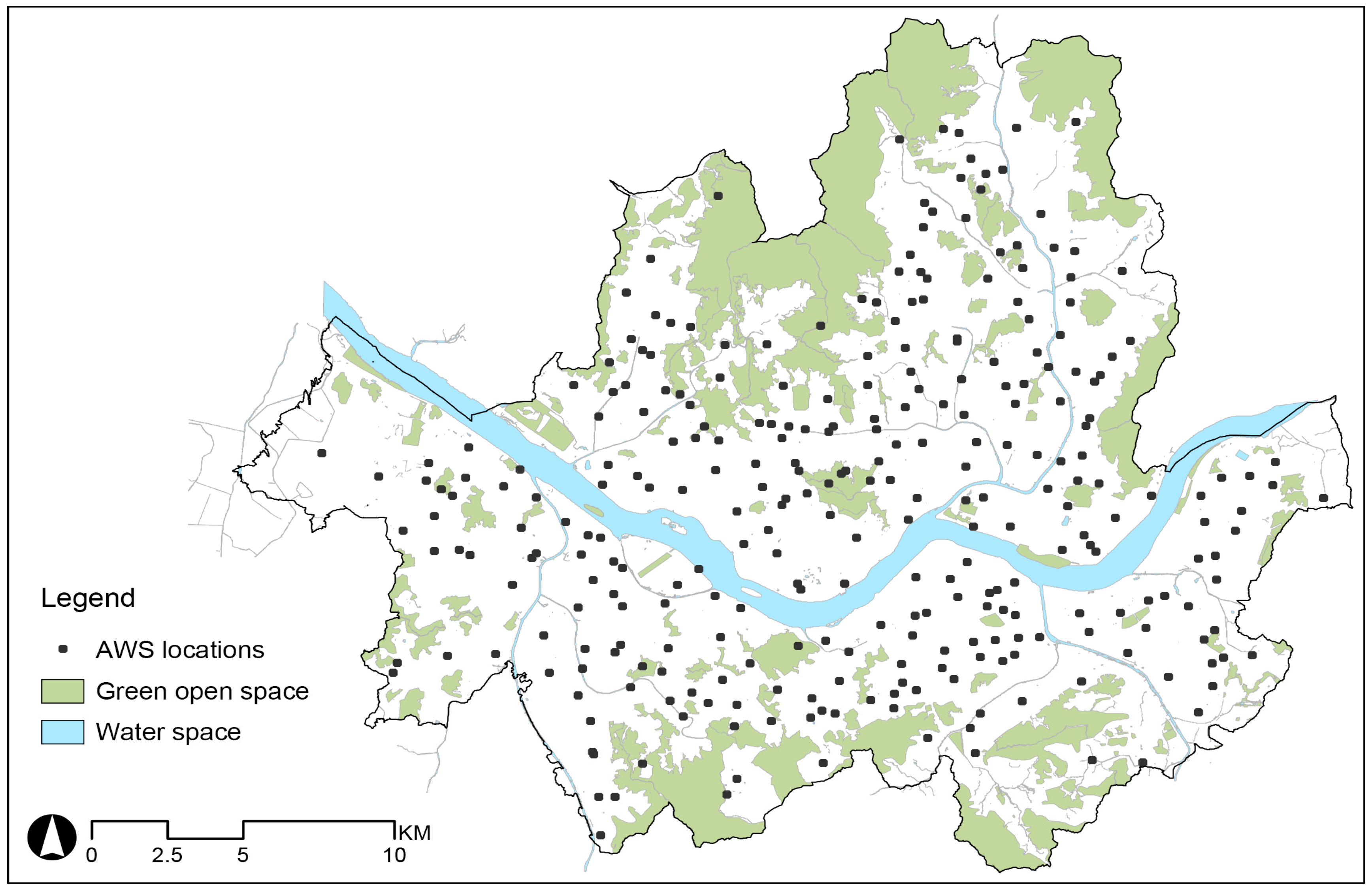
3.1. Study Area

This research focuses on Seoul, the capital city of South Korea, which is densely built, includes three central business districts (CBD) and residential areas with various housing types (see Figure 1). Seoul, with an area of 605.28 km², accommodates more than 10 million people. Recently, high air temperatures and UHIs have been critical issues in Seoul, because of global climate change and increased CO₂ emissions from traffic, households, urban facilities, etc. In effect, Seoul’s annual average air temperature has increased by 1.5 °C during the past four decades, and the UHI effect has been observed in the main CBDs. In addition, the number of patients who suffered heat-related diseases in summer increased from 556 to 1056 between 2014 and 2015 according to a report by the Korean Centers for Disease Control and Prevention [26].

We have several reasons for modelling air temperature by focusing on the SVF in Seoul. First, Seoul is an appropriate area for examining the relationship between SVF and air temperature because SVF is considered as an important variable in explaining air temperatures in high-rise, high-density urban environments. Second, because the Seoul metropolitan area is one of the highest populated urban areas in the world [27], its demand for urban guidelines to mitigate UHIs is increasing. Third, the severity of high air temperatures and UHIs has increased during the past few decades in Seoul and is now handled through government policies. Fourth, the characteristics of the built and natural environments in Seoul vary by area, which means that it is possible to model the urban temperature with various sample types. The Han River flows from the east to the west of Seoul, and natural green parks with mountains are located in the north and south. In addition, different types of business districts and residential areas are distributed throughout Seoul, making Seoul appropriate for studying the relationship between built environments and air temperature.

3.2. Variables

To model the air temperature in Seoul, we used observations from 295 AWS as the dependent variable. Of those AWS, 240 are operated by the SK Weather Planet (SKP) company, 26 are managed by the Seoul Metropolitan Government (SMG), and 29 are managed by the Korean Meteorological Administration (KMA). In terms of data reliability, SMG and KMA are public organizations that operate the AWS to collect and provide weather information using standard equipment [28,29]. We deemed the SKP data to also be reliable because SKP provides its data to public organizations [30], including the National Disaster Management Institute of Korea.

We used the air temperature observed every hour on the hour on 11 July 2015. This day showed the highest air temperature in 2015, between 25.7 °C and 36.0 °C. Furthermore, to model the air temperature during both day and night, we used the average air temperature observed during the day and night as the dependent variable for each model. In this study, we designated 10:00 to 18:00 and 22:00 to 06:00 as day-time and night-time, respectively.

We selected the independent variables for this research based on the main purpose of this study. Because modelling air temperature carries no obvious set of variables, we selected the following data by considering our objective and sample data available: (1) AWS elevation; (2) climate properties, including wind velocity and humidity; (3) SVF, directly calculated by the urban geometry; (4) solar radiation, indirectly related with the urban geometry; (5) factors known to mitigate high air temperatures, including surface albedo and proximity to natural green parks and water; (6) road area and width; and (7) gross floor area dedicated to residential and non-residential uses. We calculated the variables for a 500 m buffer area around each AWS. Most previous research on urban air temperature or UHIs has used surface temperatures extracted from Landsat TM; instead, we use observed air temperature. For this study, we decided that urban factors inside the 500 m buffer for each AWS point exert influence on the air temperature. The base year for the datasets used is 2015, except for albedo, which was extracted from the 30 May 2014, Landsat TM satellite image because of a data collection problem. Next, we provide detailed descriptions of our process for calculating each variable.

First, we collected the elevation data of each AWS managed by SKP and KMA based on the manual provided by those institutions. SMG, however, did not provide the elevation of its AWS equipment. Therefore, we calculated the elevation of those 26 AWS from the altitude, building height, and AWS height at each location. We log transformed the elevation variable for the models because the distribution of the data was right-skewed. Second, we collected datasets of climate properties such as air temperature, wind velocity, and humidity from the 295 AWS. We used the average wind speed and humidity for day and night. However, 11 stations were missing humidity values and were excluded from the modelling process. Third, we computed variables such as SVF and solar radiation using a 3D GIS dataset for Seoul, Korea. We used the “skyline” and “skyline graph” functions of the 3D Analyst Tools in the ArcGIS (ESRI, Redland, United States) for SVF computation. Most previous studies on SVF have used either the photographic or software method to determine SVF. The photographic method uses a fish-eye lens to project the hemispheric environment onto a circular plane, which enables consideration of real cases including vegetation information and irregular building shapes. However, this method requires photographs of every location for observation. For this research, we concluded that the fish-eye method was inappropriate for determining SVF because of the time and cost required. On the other hand, the software method rapidly computes SVF for many locations with a 3D GIS dataset, even if it is not as accurate as the fish-eye method.

Computing SVF via software was first proposed by Gal et al. as an extension that works in the ArcView program, and it has been used frequently in research on the relationship between SVF and air temperature [31]. Verification of the accuracy of this extension and other software, such as SOLWEIG, was conducted by Hämmerle et al. [32]. His results showed that the SVF values calculated using the photographic method and the software method have a high correlation, thereby validating the software methods. Moreover, Chen et al. compared SVF values calculated by the photographic and software methods and found a measurement error between 0.006 and 0.048, also confirming the reliability of software methods in calculating SVF [2].

We adopted the software method to compute SVF in the 500 m buffer area drawn for each 295 AWS points for this research. The 3D geometry dataset was built using the digital elevation model (DEM) and the building. To measure SVF around each AWS point, we calculated the SVF value for each point created on the road area using the ‘fishnet’ function of ArcMap 10 (see Figure 2). The method of measuring SVF using the average value of a specific area was suggested by Unger [13]. According to his research, the areal average of SVF is more appropriate than the value calculated on one specific point when modelling the relationship between temperature and SVF.

The procedure for computing the SVF at every AWS point is shown in Figure 2. First, we created a 500 m buffer area for every AWS location. Second, using the “fishnet” tool in ArcMap 10 software, we generated a 50 m grid point. Third, using the intersection geo-processing tool, we selected the grid points on the road area and excluded the grid points on the building layer. Finally, we calculated the SVF value for each point using the ‘skyline’ tool, which requires the designation of a radius. In this step, we adopted the research results of Chen et al., which suggest that 500 m is sufficient to minimize both the measurement error and the computing time [2]. Figure 3 shows example cases of the measured SVF and the bird-eye view by the areal FAR. As seen in Figure 3, the FAR decreases from (a) to (d), while the measured SVF increases from (a) to (d).

We computed the solar radiation value of each buffer area using the solar radiation tool in ArcMap 10, which analyzes the amount of solar radiation over a surface area for a specific time period. We set the latitude as 37.541, which is the latitude value of the centroid of our study area, and the analysis period as 00:00–24:00 11 July 2015, to match our climate observation. We used the total surface solar radiation to examine the relationship between solar radiation and air temperature during both day and night. As an input to the solar radiation analysis tool, we used the DEM dataset and the 3D urban model of Seoul, transforming the raster size to 2 m × 2 m and zonally averaging the raster values according to the 500 m buffer areas.

We calculated the surface albedo using the Landsat8 TM image file recorded on 30 May 2014, and algorithms developed by Liang [33]. Conforming to the algorithm, we used the digital numbers (DN) of the Landsat8 TM bands 2, 4, 5, 6, 7 to the top of atmosphere reflectance. These converted reflectance values were then used to calculate the surface albedo according to the formula presented by Smith [34]. We used albedo to control the relationship between solar radiation and air temperature. Albedo, which is described as the average reflectance of the sun’s spectrum, has values between 0 to 1.0 that vary according to land cover.

The proximity of each AWS location to green open spaces or the river were used to control for the effect of vegetation and water on air temperature. Merging the layers of green open spaces in the north and south and the Han River crossing from east to west in Seoul, we used the “generate near table” tool in ArcGIS. We calculated the average width and total area of the roads that intersect each 500 m buffer around AWS locations with road GIS data. We used the average road width in each buffer to control the relationship between SVF and air temperature. For example, even if the SVF values for two buffers are equal, the forms of the buildings and roads could be different. We included the road area variable because roads in Seoul have critical effects on air temperature due to their impervious surface, heat-absorbing properties, and traffic.

Land use measurements included building gross floor area (GFA) for residential and non-residential uses. We calculated these indices based on the 500 m buffers from each AWS point. We converted the value using a log transformation because the data showed positive skewness.

The descriptive statistics for the variables are shown in

Table 1. Descriptive statistics.

Variables			Avg.	S.D.	Min.	Max.
Name		Unit
Daytime	Average air temperature	°C	32.881	0.573	30.267	34.378
	Average wind velocity	m/s	2.054	0.718	0.567	4.478
	Average humidity	%	57.285	4.955	22.256	100.000
Night-time	Average air temperature	°C	27.263	0.826	22.756	29.244
	Average wind velocity	m/s	1.404	0.745	0.056	5.067
	Average humidity	%	77.923	5.368	41.563	100.000
Elevation of AWS equipment		m	58.901	28.078	5.000	332.000
Surface solar radiation		MJ/m2	4577.233	403.078	3575.350	5736.520
Sky view factor		-	0.599	0.100	0.419	0.991
Surface albedo		-	0.152	0.008	0.122	0.177
Average road width		m	8.031	3.519	2.991	32.601
Total road area		m2	157,902.492	49,138.687	2322.402	266,401.380
Residential GFA		m2	75,133.672	47,461.875	0.000	223,230.975
Non-residential GFA		m2	93,018.269	107,673.248	0.000	874,794.593
Proximity to open space		m	1056.301	780.038	0.000	3546.934

. Before the analysis, we conducted a log transformation on elevation, solar radiation, road width and area, gross floor area (GFA) for residential and non-residential uses, and proximity to open spaces to adjust them to a normal distribution.

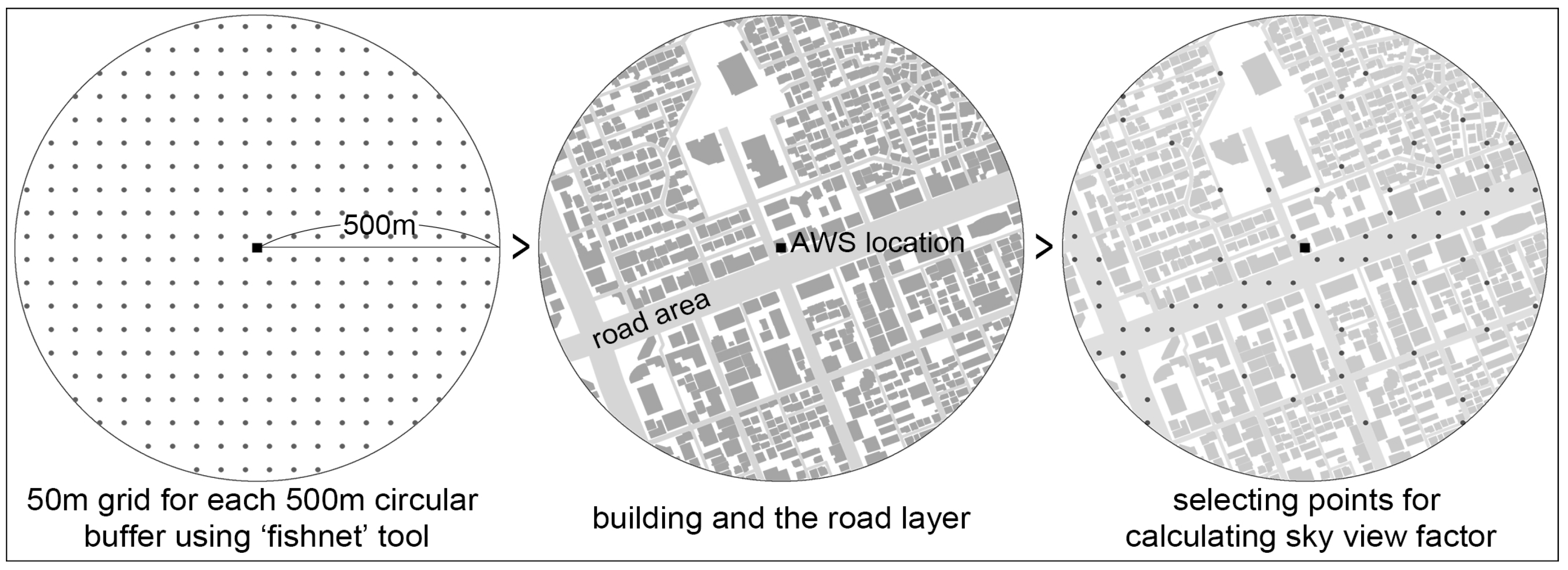
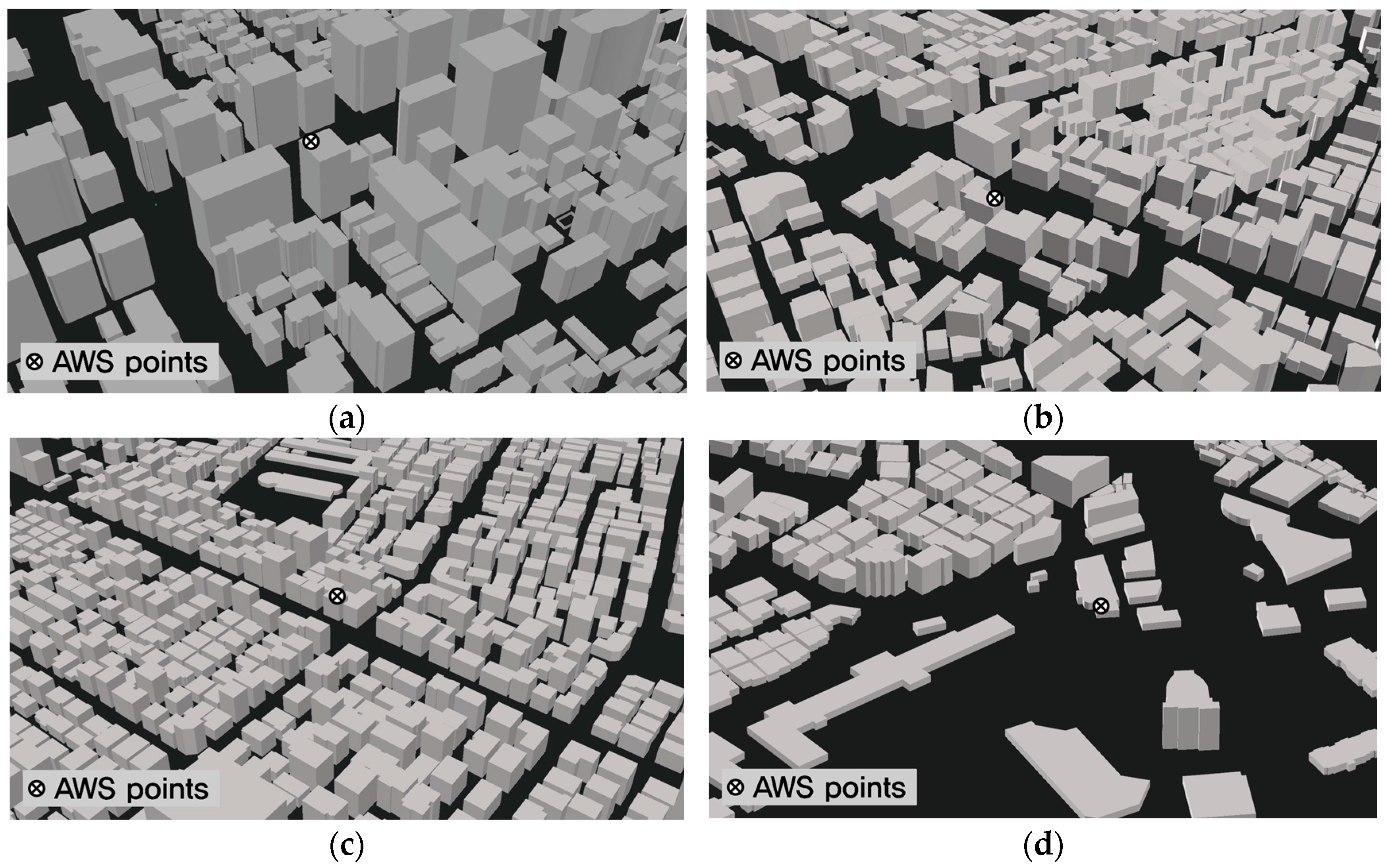
3.3. Research Process and Methodology

Our first step was to examine the relationship between air temperature and SVF during the day and night. We used a regression model to control other environmental factors that could affect air temperature. To derive the estimation method that best explains air temperature, we built an ordinary least squares (OLS) model and a spatial regression model. We verified the spatial autocorrelation of observed air temperature between a specific AWS location point and its neighboring AWS using the Moran’s I indices provided by the GeoDa software. According to previous studies, the spatial regression model is appropriate for estimating temperature because temperature has a tendency to be spatially correlated with the temperature observed nearby due to atmospheric flows [1]. Using OLS in modelling the air temperature, an analysis error can result from the spatial dependency and heterogeneity of the spatial data.

In the next step, we examined the relationship between air temperature and SVF according to the FAR of the study area. The purpose of this step was to analyze the value of FAR, when the effect of SVF on air temperature is maximized. An equal amount of change in SVF can affect air temperature differently according to the areal FAR. Therefore, we sorted our 284 AWS samples in descending order of FAR value. Then we selected 150 samples progressively, creating 135 datasets. Next, we generated an OLS model for each of the 135 datasets using the dependent variable of air temperature at daytime or nighttime and other independent variables. Based on the regression results, we extracted the coefficient value of the SVF variable to examine its changing effects with air temperature as the areal FAR increases during both day and night.

4. Analysis, Results, and Interpretations

The analysis results and interpretations will be in three parts. The first and the second parts will discuss the association between the urban indices and the air temperature observed during the day and night using regression models. In this step, we used the Moran I test to identify whether spatial autocorrelation exists in the dependent variable or in the residuals (error terms). We created the spatial weight matrix W using the distance weight option in the GeoDa software. We set the threshold distance at the default value provided by the software, which is the minimum threshold distance available. We decided whether to use a spatial regression model according to the results of the Moran I test. The spatial autocorrelation effect is captured using spatial regression models, such as the spatial lag model (SLM) and the spatial error model (SEM). In addition, we used SEM with KP-Het option in the GeoDa Space software to capture the presence of heteroscedasticity. Analysis results for day and night are shown in Section 4.1 and Section 4.2, respectively.

The third part discusses the changing relationship between SVF and air temperature according to the FAR of the study area from the 135 OLS models for day and night. Analysis results are described in Section 4.3. We performed this step to understand the effect of SVF on air temperature as FAR varies. While we focused on SVF, we used the other urban indices in modelling the air temperature as control variables.

4.1. Part 1: Effect of Urban Indices on Daytime Air Temperature

Table 2. Analysis results of the influence factors on air temperature (daytime).

Variable Description	OLS Model		Spatial Lag Model		Spatial Error Model		Spatial Error Model with KP-Het
	Coef.	t	Coef.	z	Coef.	z	Coef.	z
(Constant)	28.335 ***	7.05	24.609 ***	5.54	28.744 ***	7.30	28.567 ***	6.72
Elevation	−0.184 ***	−3.18	−0.209 ***	−3.69	−0.231 ***	−4.05	−0.218 ***	−2.91
Wind Velocity	−0.299 ***	−8.33	−0.292 ***	−8.31	−0.295 ***	−8.39	−0.296 ***	−7.62
Humidity	−0.038 ***	−6.78	−0.036 ***	−6.74	−0.034 ***	−6.29	−0.035 **	−2.56
Surface Solar Radiation	0.861 *	1.79	0.790 *	1.68	0.856 *	1.81	0.863 *	1.73
Sky View Factor	−1.462 ***	−3.00	−1.406 ***	−2.95	−1.464 ***	−3.07	−1.473 ***	−3.65
Surface Albedo	−3.107	−0.78	−2.765	−0.71	−5.103	−1.28	−4.474	−1.13
Road Width	0.266 ***	2.79	0.227 **	2.41	0.214 **	2.17	0.229 **	2.29
Road Area	0.120 **	2.20	0.119 **	2.25	0.120 **	2.25	0.121 ***	2.97
Residential GFA	0.023	1.10	0.021	1.01	0.024	1.17	0.025	1.13
Non-residential GFA	−0.037	−1.29	−0.035	−1.26	−0.034	−1.2	−0.036 *	−1.66
Proximity to Open Space	0.046 *	1.81	0.042 *	1.68	0.045 *	1.71	0.045 **	2.00
Wy			0.133 *	1.74
Lambda(λ)					0.241 ***	2.64	0.216 **	2.57
Moran’s I	0.074 ***		0.019		−0.007		n/a
Jarque-Bera test	24.809 ***
Breusch-Pagan test	25.181 ***		25.623 ***		20.847 **		n/a
LM-test			3.495 *		4.780 **		n/a
N	284		284		284		284
R-squared	0.519		0.526		0.533		0.518
LR-test			3.098 *		5.284 **		n/a
AIC	305.0		303.9		299.7		n/a
SC	348.7		351.3		343.5		n/a

*** p < 0.01; ** p < 0.05; * p < 0.10.

presents the effect of urban environments on daytime air temperature using an OLS model, SLM, SEM, and SEM with KP-Het option. Before discussing the relationship between independent variables and air temperature, the Jarque-Bera test shows that the sample data do not match the normal distribution. In addition, the results of the Breusch-Pagan test indicate heteroscedasticity in the model estimation. The Moran’s I value for the OLS model (Table 2) is statistically significant, which implies that the error terms of the OLS model are spatially autocorrelated. Because of the Moran’s I value, spatial regression models were used to capture and reduce the degree of spatial autocorrelation. Furthermore, we conducted SEM with KP-Het option to capture the heteroscedasticity of the model.

According to the Lagrange multiplier value computed for the SLM and SEM, SEM was more suitable for modelling air temperature. In addition, because the R-squared value is inappropriate for identifying the goodness of fit for spatial regression models, we used the log-likelihood ratio (LR test), Akaike information criterion (AIC), and Schwarz criterion (SC) to select the final model. Referring to Anselin [35], high LR-test values and low AIC and SC values indicate a well-estimated model. Hence, we focused on the SEM results. Furthermore, we examined the results of the model with the KP-Het option activated. The estimated results between models, however, did not present any striking differences, as described in Table 2.

Focusing on the SEM results, variables related to the AWS (control variables) were statistically significant to daytime air temperature. Coefficient directions of the elevation of the AWS, wind velocity, and humidity agree with the results of previous studies. In addition, the coefficients of those variables were statistically significant at the 1% level and negative. For solar radiation, the coefficient was statistically significant at the 10% level (marginal) and positive. These results agree with the theory that a higher amount of solar radiation causes an increase in daytime air temperature.

The coefficient of the SVF, which is the main focus in this study, had a negative relationship with the daytime air temperature and was statistically significant at the 1% level. This result contributes to the literature by adding a case study about the relationship between SVF and daytime air temperature. As addressed in the literature review part, relationship between SVF and daytime air temperature can be either positive or negative, depending on the characteristics of the study area [2].

In principle, as Giridharan et al. stated, SVF should have a positive effect on air temperature [8,17,23]; however, the regression coefficients of our research support the opposite case. According to Giridharan et al., urban areas with more visible open sky view have higher urban air temperatures because of a larger solar radiation effect increasing air temperature. On the other hand, there are also studies reporting opposite results, which argue that an increase in SVF leads to a decrease of daytime air temperature [1,2]. Chen et al. found a negative relationship between SVF and daytime air temperature [2]. Although they admitted that the ‘negative’ relationship was not clearly addressed, they explained this result through differences in the study area. Chen et al. also mentioned that the research of Giridharan et al. was more focused on high-rise and high-density built environments, which produce a different outcome. Therefore, the effect of SVF on daytime air temperature is still a debatable issue. Our study indicated that the coefficient of SVF showed negative association with air temperature, which implies lower air temperature with more visible open sky view, capturing the effects of wind velocity, solar radiation, and albedo. While an increase in SVF leads to an increase in solar radiation that is associated with an increase of air temperature, it also leads to higher level of air circulation that may decrease air temperature. The negative association between SVF and air temperature seen in our study indicates that the air circulation effect with higher SVF plays a role in lowering air temperature.

Surface albedo had a negative coefficient, meaning that an increase in surface albedo leads to a decrease in air temperature. This results agree with the general theory; however, our finding was not statistically significant. Meanwhile, urban indices related to roads, such as road width and road area, showed a positive relationship with daytime air temperature, in accordance with both previous results and theory. In the SEM, both road width and road area were statistically significant at the 5% level. The coefficient of the GFA calculated for both residential and non-residential use was not statistically significant. Few previous results have verified whether a difference in building use affects surface temperature; however, we found that it was not a significant variable because our temperature data were observed by AWS rather than satellite images. Distance-based proxy variables for natural open spaces such as a mountain or the river were significant and positive. This means that an increase in the distance to a natural open space leads to an increase in air temperature, falling in line with the general UHI theory.

Overall, the results of the influence factors on air temperature generally matched the theoretical concepts. We solved the spatial autocorrelation shown in the OLS model by referring to Moran’s I value and the lambda coefficient in the SEM. We also built a SEM activating the KP-het option; however, it did not show a large difference with the original SEM result.

4.2. Part 2: Effect of Urban Indices on Night-Time Air Temperature

Table 3. Analysis results of the influence factors on air temperature (night time).

Variable Description	OLS Model		Spatial Lag Model		Spatial Error Model		Spatial Error Model with KP-Het
	Coef.	t	Coef.	z	Coef.	z	Coef.	z
(Constant)	24.931 ***	4.63	12.527 ***	2.82	28.900 ***	6.89	28.077 ***	6.43
Elevation	0.131 *	1.75	0.065	1.07	0.062	1.05	0.076	1.33
Wind Velocity	−0.015	−0.34	−0.009	−0.25	−0.029	−0.83	−0.027	−0.78
Humidity	−0.077 ***	−10.96	−0.054 ***	−9.04	−0.049 ***	−8.04	−0.054 ***	−4.78
Surface Solar Radiation	1.123 *	1.75	0.394	0.76	0.284	0.57	0.431	0.84
Sky View Factor	−1.343 **	−2.07	−1.142 **	−2.18	−1.353 ***	−2.67	−1.381 **	−2.00
Surface Albedo	−25.343 ***	−4.68	−12.856 ***	−2.86	−16.735 ***	−3.79	−17.828 ***	−3.82
Road Width	0.121	0.96	0.148	1.46	0.163	1.42	0.179	1.34
Road Area	0.142 *	1.95	0.088	1.50	0.087	1.55	0.091	1.52
Residential GFA	−0.003	−0.12	0.024	1.06	0.037 *	1.69	0.034 *	1.71
Non−residential GFA	0.036	0.92	0.034	1.10	0.041	1.36	0.040	1.49
Proximity to Open Space	0.114 ***	3.37	0.077 ***	2.78	0.110 ***	3.41	0.114 ***	3.25
Wy			0.567 ***	12.46
Lambda(λ)					0.721 ***	14.96	0.697 ***	15.18
Moran’s I	0.350 ***		0.058 *		−0.016		n/a
Jarque-Bera test	62.957 ***
Breusch-Pagan test	29.350 ***		46.721 ***		37.924 ***		n/a
LM-test			100.676 ***		106.125 ***		n/a
N	284		284		284		284
R-squared	0.594		0.725		0.744		0.572
LR-test			92.127 ***		98.164 ***		n/a
AIC	464.2		374.0		366		n/a
SC	508.0		421.5		409.8		n/a

*** p < 0.01; ** p < 0.05; * p < 0.10.

shows the associations between urban indices and nocturnal air temperature. For this part, we analyzed the four models as described in Section 4.1. The OLS model on nocturnal air temperature showed that the sample data were not normally distributed and that the error terms of the model have propensity for heteroscedasticity.

The Moran’s I value of the OLS model was 0.350, which is significant at the 1% level. This indicates that the error terms of the nocturnal air temperature model are spatially autocorrelated to a higher degree than those in the daytime air temperature model. To capture and reduce the spatial autocorrelation, we used the LM-test to select the final model between the SLM and SEM. The indicators of the LM-test showed that the SEM is more appropriate than the SLM in modelling the nocturnal air temperature, which is the same as modelling the daytime air temperature. The LR-test value was the highest, and AIC and SC were the lowest in the SEM, implying that the SEM has the highest goodness of fit among the models. In addition, the Moran’s I value of the SEM was not statistically significant, indicating that the spatial autocorrelation of the OLS model was fully captured. Hence we selected the SEM as the final model and described its results below.

The coefficients of the variables related to the AWS were different from for daytime air temperature. Elevation of the AWS and wind velocity were not statistically significant, which implies that these environmental indices are only related to daytime air temperature. On the other hand, humidity was statistically significant at the 1% level and negative. This result does not present a large difference from the daytime air temperature case. The coefficients for solar radiation were not statistically significant in the SEM results, but they were significant in the OLS model. This demonstrates that results can vary if the spatial autocorrelation of the sample data is not properly addressed, which can cause false results to a certain degree.

The association between SVF and nocturnal air temperature was negative and statistically significant at the 1% level. This result falls in line with the general theory, which is that an increase in SVF normally results in a decrease in night air temperature. The negative coefficient of SVF indicates that higher air temperature is associated with lower SVF. Moreover, the areas with lower SVF are mostly urban centers, which is consistent with UHI theory. In summary, the coefficient of SVF in both the day and night models were negative with strong statistical significance. The results of our study are important because we provided the regression coefficient of SVF on air temperature for both the day and night, capturing the effects of wind velocity and solar radiation with sufficient sample size. Therefore, our study confirms that SVF has a negative effect on both day and night air temperatures, although the coefficient of SVF in the daytime was slightly stronger than in nighttime. However, it should be noted that these results can only be applicable in our study area in Seoul.

Surface albedo showed a strong negative effect on nocturnal air temperature significant at the 1% level. This result differs from the daytime air temperature model, in which the coefficient of the surface albedo was not significant. Meanwhile, the coefficients of the road variables were not statistically significant, which also differs from the result of the daytime model, where they showed statistical significance. The coefficients of the GFA for residential uses were positive and showed significance at the 10% level. This result contrasts with the daytime model, which showed no significance. On the other hand, the coefficients of the GFA for non-residential uses did not show significance, which agrees with the daytime model results.

The coefficients of the proximity to open space were positive and showed statistical significance at the 1% level. This result accords with the theory, which implies that the air temperature increases as the distance from natural open spaces gets higher. Overall, the analysis results of the urban indices on nocturnal air temperature showed some differences with the results for daytime air temperature.

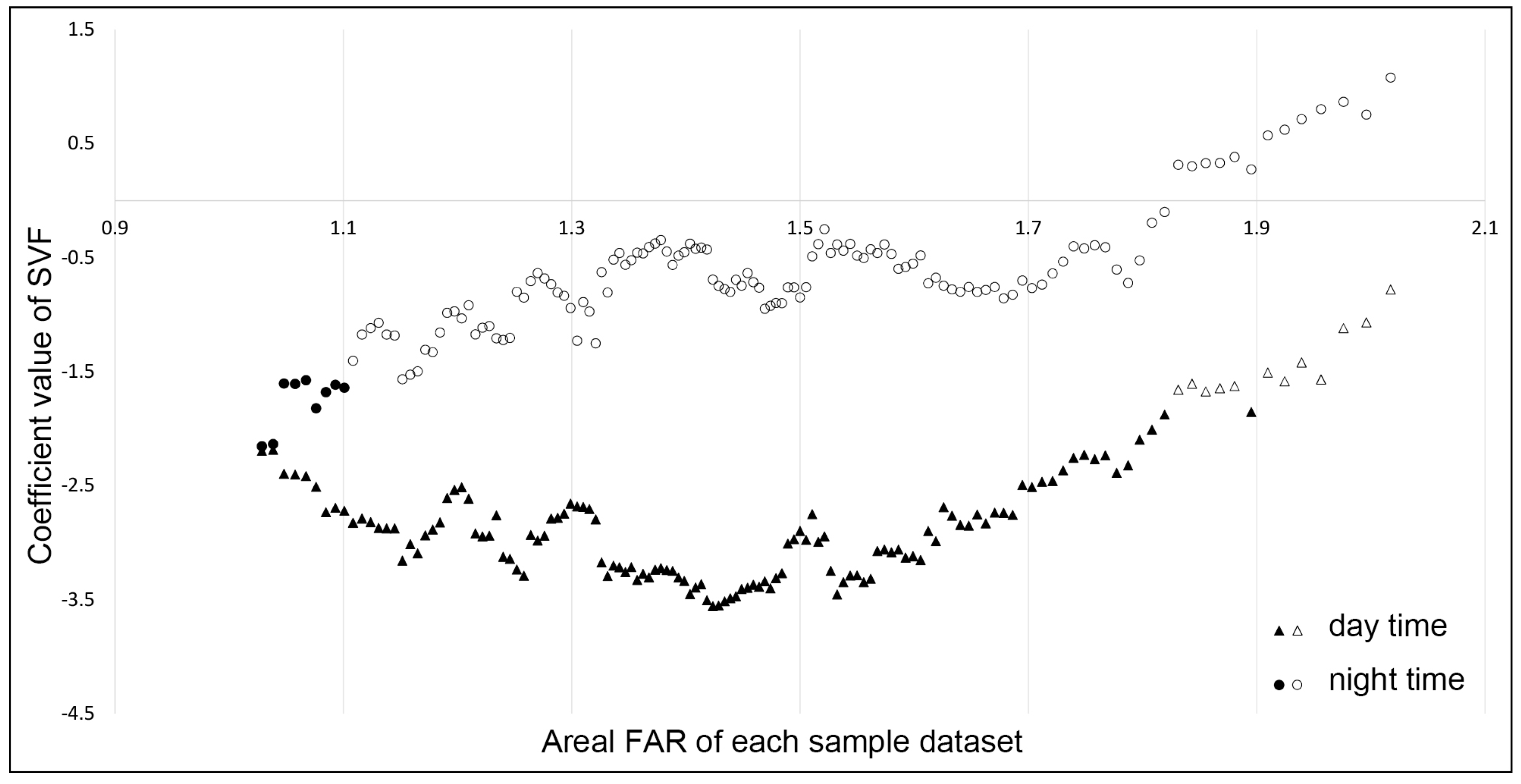
4.3. Part 3: Changing Effect of SVF on Day and Night Air Temperature by FAR

We analyzed the changing effects of SVF on day and night air temperatures according to the FAR of the area. To do so, we built an OLS model for samples selected according to the areal FAR. We created 135 datasets by selecting 150 samples from 284 samples, according to the areal FAR value of each sample. Using those datasets, we conducted 135 regression analyses, using the control variables explained in the prior section. We then extracted the coefficient and the probability value of the SVF estimated for each analysis. Based on the results of this section, we expect that planners and policy makers will be able to make decisions on where to adjust or regulate the value of SVF to mitigate UHI intensity.

The changing pattern of SVF coefficients on air temperature along with FAR in the day and night are shown in Figure 4. The y-axis presents the coefficient values of SVF from regression models and the x-axis shows the average areal FAR value of the dataset used in each analysis. Moreover, the color of the point indicates the statistical significance. Black indicates a statistical significance at the 90% confidence level, white indicates no significance. For example, the coefficient value of SVF is approximately −3.5 at day time and −0.5 at night time, when the average FAR of the selected samples is slightly above 1.4 (see Figure 4).

As seen in Figure 4, the SVF coefficient shows a U-shaped pattern in the daytime. The coefficient value decreases until the average FAR reaches about 1.5 and then increases as the areal FAR rises. This implies that the effect of SVF on air temperature is strong in areas where the areal FAR is 1.5 and weakens when the average FAR increases or decreases. At some points, especially when the average FAR of the regression sample is high, the SVF coefficient did not show statistical significance at the 90% confidence level. The reason for the U-shaped pattern of the SVF coefficient at daytime is not obvious. However, we hypothesize that it is attributed to the following aspect. In general, SVF is associated with wind velocity, which promotes air circulation. As a result, larger SVF with higher levels of air circulation leads to a decrease in air temperature. Meanwhile, according to Yang et al., wind velocity decreases as the FAR increases [36]. Therefore, we conclude that the effect of SVF for enhancing air circulation decreases in urban areas where FAR is high. On the other hand, we speculate that solar radiation will be higher in areas with low FAR. As Giridharan et al. stated, the increase of SVF leads to an increase in daytime air temperature due to higher solar radiation [8]. However, solar radiation is expected to be low in surfaces with higher FAR due to building footprints or shadows. Therefore, it can be argued that the coefficient of SVF in areas of lower FAR increases due to the counterbalance of solar radiation. However, future research should clarify this issue.

In the analysis of nocturnal air temperature, most of the SVF coefficient values were not statistically significant. Only a few of the regression samples, mostly conducted in areas with low areal FAR, showed significance. However, it is obvious that the pattern of the nocturnal SVF coefficient values differs from the daytime analysis. As seen in Figure 4, the SVF coefficients from night-time air temperature tended to increase steadily from approximately −1.5 to 1.0. This indicates that the effect of SVF on nocturnal air temperature changes from negative to positive as the areal FAR of the study area increases. However, it is difficult to be certain about the observed patterns because most of the results were not statistically significant at the 10% level.

Comparing the SVF coefficient values between day and night, the greatest difference was found when the areal FAR was approximately 1.5. This gap decreased with the average FAR of the study area. On the other hand, the gap maintained its size as the average FAR increased to about 2.0. The analysis results in Figure 4 are not certain because of the degree of significance; however, they do indicate differences in the SVF coefficient value during day and night. We expect our analysis results on the relationship between SVF and FAR to be complemented by further studies. Previous studies have implied that SVF can be an important factor in analyzing the air temperature in high-rise, high-density areas, but they have not suggested sufficient reason for this occurrence.

5. Conclusions

In this study, we analyzed the relationships between air temperature and urban environmental indices, mainly focusing on SVF. In doing so, we used day-time and night-time air temperatures, collected from 295 AWS in Seoul, as the dependent variable. In addition, by selecting samples according to the areal FAR, we identified the changing effects of SVF on air temperature. Moreover, we used spatial regression analysis to capture the effect of the spatial autocorrelation detected in our spatial data.

Our findings indicated that SVF negatively affects air temperature during both day and night when other effects are controlled through regression analysis. Comparing this result with previous research on the relationship between SVF and air temperature, we found different results regarding the daytime SVF regression coefficient [8]. However, our results agree with other research that has asserted that the coefficients of SVF can be either positive or negative when modelling daytime air temperature [2]. Moreover, the results of our study were robust with advanced methodology and a sufficient number of samples, while capturing the effect of wind velocity and spatial autocorrelation.

Overall, our study shows that environmental indices affect day and night air temperature differently. Elevation of the AWS and wind velocity negatively affect air temperature, whereas solar radiation, road width, and road area positively affect daytime air temperature. In contrast, surface albedo showed a strong association with nocturnal air temperature. This finding indicates that different environmental indices should be considered when mitigating daytime or night-time air temperatures. In addition, humidity, SVF, and proximity to open space play important roles during both day and night.

Furthermore, we discovered patterns in the SVF coefficient when changing the analysis dataset according to the areal FAR. The relationship between SVF and daytime air temperature showed a U-shaped curve as the areal FAR increased, with most results being significant. While the SVF regression coefficients at night time were mostly not significant, they showed an increasing pattern as the areal FAR increased. These findings are meaningful because they imply that SVF can have different associations with air temperature according to the areal FAR. In addition, our findings will assist planners and policy makers developing policy priorities to mitigate UHI with regard to SVF.

This study contributes to the literature on the relationship between SVF and air temperature observed during the day and night in high-rise, high-density cities. However, it should be noted that this research has a few limitations. Because the SVF coefficients for night-time air temperature according to the FAR were not significant, the result offers limited confidence. Therefore, additional research should address the relationship between SVF and air temperature while considering the FAR of the research area. In this study we were also unable to address various environmental indices that are known to affect air temperature, such as traffic volume and heat sinks. Thus, further research should resolve those limitations using variables that can better explain air temperature.

References

1. Chun, B.S.; Guldmann, J.M. Spatial statistical analysis and simulation of the urban heat island in high-density central cities. Landsc. Urban Plan. 2014, 125, 76–88. [Google Scholar] [CrossRef]
2. Chen, L.; Ng, E.; An, X.; Ren, C.; Lee, M.; Wang, U.; He, Z. Sky view factor analysis of street canyons and its implications for daytime intra-urban air temperature differentials in high-rise, high-density urban areas of Hong Kong: A GIS-based simulation approach. Int. J. Climatol. 2012, 32, 121–136. [Google Scholar] [CrossRef]
3. Oke, T.R. The energetic basis of the urban heat island. Q. J. R. Meteorol. Soc. 1982, 108, 1–24. [Google Scholar] [CrossRef]
4. Wong, N.H.; Yu, C. Study of green areas and urban heat island in a tropical city. Habitat Int. 2005, 29, 547–558. [Google Scholar] [CrossRef]
5. Solecki, W.D.; Rosenzweig, C.; Parshall, L.; Pope, G.; Clark, M.; Cox, J.; Wiencke, M. Mitigation of the heat island effect in urban New Jersey. Glob. Environ. Chang. Part B Environ. Hazards 2005, 6, 39–49. [Google Scholar] [CrossRef]
6. Pyun, H.S.; Song, Y.B.; Han, B.H. Landuse planning method considering urban greenery and urban climate. J. Korea Plan. Assoc. 2009, 44, 37–49. [Google Scholar]
7. Cha, Y.H.; Kim, H.Y.; Heo, T.Y. The effects of urban land use and land cover characteristics on air temperature in Seoul Metropolitan area. Seoul Stud. 2009, 10, 107–120. [Google Scholar]
8. Giridharan, R.; Lau, S.S.Y.; Ganesan, S.; Givoni, B. Lowering the outdoor temperature in high-rise high-density residential developments of coastal Hong Kong: The vegetation influence. Build. Environ. 2008, 43, 1583–1595. [Google Scholar] [CrossRef]
9. Yeo, I.A.; Yee, J.J.; Yoon, S.H. Analysis on the effects of building coverage ratio and floor space index on urban climate. J. Korean Sol. Energy Soc. 2009, 29, 19–27. [Google Scholar]
10. Kim, Y.; An, S.M.; Eum, J.H.; Woo, J.H. Analysis of thermal environment over a small-scale landscape in a densely built-up Asian megacity. Sustainability 2016, 8, 358. [Google Scholar] [CrossRef]
11. Yuan, J.; Emura, K.; Farnham, C. Highly reflective roofing sheets installed on a school building to mitigate the urban heat island effect in Osaka. Sustainability 2016, 8, 514. [Google Scholar] [CrossRef]
12. Kakon, A.N.; Nobuo, M. The sky view factor effect on the microclimate of a city environment: A case study of Dhaka City. In Proceedings of the 7th International Conference on Urban Climate, Yokohama, Japan, 29 June–3 July 2009.
13. Svensson, M.K. Sky view factor analysis—Implications for urban air temperature differences. Meteorol. Appl. 2004, 11, 201–211. [Google Scholar] [CrossRef]
14. Unger, J. Modelling of the annual mean maximum urban heat island with the application of 2 and 3D surface parameters. Clim. Res. 2006, 30, 215–226. [Google Scholar] [CrossRef]
15. Unger, J. Intra-urban relationship between surface geometry and urban heat island: Review and new approach. Clim. Res. 2004, 27, 253–264. [Google Scholar] [CrossRef]
16. Chun, B.S.; Kim, H.Y. Analysis of urban heat island effect using information from 3-dimensional city model. J. Korea Spat. Inf. Soc. 2010, 18, 1–11. [Google Scholar]
17. Giridharan, R.; Ganesan, S.; Lau, S.S.Y. Daytime urban heat island effect in high-rise and high-density residential developments in Hong Kong. Energy Build. 2004, 36, 525–534. [Google Scholar] [CrossRef]
18. Oke, T.R. Canyon geometry and the nocturnal urban heat island: Comparison of scale model and field observations. J. Climatol. 1981, 1, 237–254. [Google Scholar] [CrossRef]
19. Barring, L.; Mattsson, J.O.; Lindqvist, S. Canyon geometry, street temperatures and urban heat island in Malmö, Sweden. J. Climatol. 1985, 5, 433–444. [Google Scholar] [CrossRef]
20. Grimmond, S. Urbanization and global environmental change: Local effects of urban warming. Geogr. J. 2007, 173, 83–88. [Google Scholar] [CrossRef]
21. Unger, J. Connection between urban heat island and sky view factor approximated by a software tool on a 3D urban database. Int. J. Environ. Pollut. 2008, 36, 59–80. [Google Scholar] [CrossRef]
22. Kim, Y.J.; Kang, D.H.; Ahn, K.H. Characteristics of urban heat-island phenomena caused by climate changes in Seoul, and alternative urban design approaches for their improvements. J. Urban Des. Inst. Korea 2011, 12, 5–14. [Google Scholar]
23. Giridharan, R.; Lau, S.S.Y.; Ganesan, S.; Givoni, B. Urban design factors influencing heat island intensity in high-rise high-density environments of Hong Kong. Build. Environ. 2007, 42, 3669–3684. [Google Scholar] [CrossRef]
24. Wang, Y.; Akbari, H. Effect of sky view factor on outdoor temperature and comfort in Montreal. Environ. Eng. Sci. 2014, 31, 272–287. [Google Scholar] [CrossRef]
25. Kubota, T.; Miura, M.; Tominaga, Y.; Mochida, A. Wind tunnel tests on the relationship between building density and pedestrian-level wind velocity: Development of guidelines for realizing acceptable wind environment in residential neighborhoods. Build. Environ. 2008, 43, 1699–1708. [Google Scholar] [CrossRef]
26. Korean Centers for Disease Control and Prevention. 2015 Annual Report on the Notified Patients with Heat-Related Illness in Korea. Available online: http://www.cdc.go.kr/CDC/info/CdcKrInfo0203.jsp?menuIds=HOME001-MNU1130-MNU1359-MNU1360-MNU1361&cid=67116 (accessed on 3 August 2016).
27. Demographia World Urban Areas. 11th Annual Edition ed. St. Louis: Demographia. Available online: http://www.demographia.com/db-worldua.pdf/ (accessed on 2 August 2016).
28. 2016 Present Conditions and Ratings of Automatic Weather System in Seoul. Available online: http://opengov.seoul.go.kr/sanction/8913777/ (accessed on 3 August 2016).
29. 2015 Standardization Level of Meteorological Observation Installations. Available online: http://web.kma.go.kr/notify/information/publication_depart_list.jsp?bid=depart&mode=view&num=200&page=1&field=&text= (accessed on 3 August 2016).
30. SKP Weather Service. Available online: http://weatherplanet.co.kr/partners/ (accessed on 1 August 2016).
31. Gal, T.; Lindberg, F.; Unger, J. Computing continuous sky view factors using 3D urban raster and vector databases: comparison and application to urban climate. Theor. Appl. Climatol. 2009, 95, 111–123. [Google Scholar] [CrossRef]
32. Hämmerle, M.; Gál, T.; Unger, J.; Matzarakis, A. Comparison of models calculating the sky view factor used for urban climate investigations. Theor. Appl. Climatol. 2011, 105, 521–527. [Google Scholar] [CrossRef]
33. Liang, S. Narrowband to broadband conversions of land surface albedo I: Algorithms. Remote Sens. Environ. 2001, 76, 213–238. [Google Scholar] [CrossRef]
34. Yale University, Center for Earth Observation. How to Convert Landsat DNs to Albedo. Available online: http://yceo.yale.edu/how-convert-landsat-dns-albedo (accessed on 2 February 2016).
35. Anselin, L. Exploring Spatial Data with GeoDa: A Work Book; Spatial Analysis Laboratory, University of Illinois, Center for Spatially Integrated Social Science: Urbana, IL, USA, 2005. [Google Scholar]
36. Yang, F.; Qian, F.; Lau, S.S. Urban form and density as indicators for summertime outdoor ventilation potential: A case study on high-rise housing in Shanghai. Build. Environ. 2013, 70, 122–137. [Google Scholar] [CrossRef]
Figure 1. The locations of 295 AWS and the natural open spaces in Seoul, Korea.
Sustainability 08 00895 g001
Figure 2. Process of selecting points for SVF calculation.
Sustainability 08 00895 g002
Figure 3. Example cases with SVF and FAR values. (a) Yeoksam-dong, Gangnam area, SVF = 0.556; FAR = 3.937; (b) Hongik Univ. station, Mapo area, SVF = 0.589; FAR = 2.463; (c) Mangwon-dong, Mapo area, SVF = 0.597; FAR = 1.718; (d) Sinrim-dong, Gwanak area, SVF = 0.678; FAR = 0.955.
Sustainability 08 00895 g003
Figure 4. Changes in the coefficient of SVF on air temperature during the day and night as FAR changes.
Sustainability 08 00895 g004