Transport Emissions and Energy Consumption Impacts of Private Capital Investment in Public Transport
by
 , and
, and
Yunqiang Xue
1,* ,
,
Hongzhi Guan
2,3, 
Jonathan Corey
4,
Bing Zhang
1,
Hai Yan
3,
Yan Han
3 and
Huanmei Qin
3 1
College of Transportation and Logistics, East China JiaoTong University, Nanchang 330013, China
2
College of Architecture and Civil Engineering, Beijing University of Technology, Beijing 100124, China
3
Beijing Collaborative Innovation Center for Metropolitan Transportation, Beijing University of Technology, Beijing 100124, China
4
ART-Engines Transportation Research Lab, University of Cincinnati, Cincinnati, OH 45220, USA
*
Author to whom correspondence should be addressed.
Sustainability 2017, 9(10), 1760; https://doi.org/10.3390/su9101760
Submission received: 30 July 2017
/
Revised: 22 September 2017
/
Accepted: 26 September 2017
/
Published: 3 October 2017
(This article belongs to the Section Economic and Business Aspects of Sustainability)
Abstract
:Introducing private capital into the public transport system for its sustainable development has been increasing around the world. However, previous research ignores emissions and energy consumption impacts, which are important for private capital investment policy-making. To address this problem, the system dynamic (SD) approach was used to quantitatively analyze the cumulative effects of different private capital investment models in public transport from the environmental perspective. The SD model validity was verified in the case study of Jinan public traffic. Simulation results show that the fuel consumption and emission reductions are obvious when the private capital considering passenger value invests in public transport compared with the no private capital investment and traditional investment models. There are obvious cumulative reductions for fuel consumption, CO2, CO, SO2, and PM10 emissions for 100 months compared with no private capital investment. This research verifies the superiority of the passenger value investment model in public transport from the environmental point of view, and supplies a theoretical tool for administrators to evaluate the private capital investment effects systematically.
1. Introduction
It has been considered common sense that public transport benefits sustainable urban development and transportation sustainability [1]. However, to keep the ticket prices at low levels, subsidies are usually needed for a public transport system. Therefore, governments at all levels have to face the problem of maintaining service quality based on limited financial resources and keeping transit fares at low levels [2,3]. Fortunately, private capital provides an alternative solution to the problem due to its financial support, efficiency, and technology advances [4].
The developed countries’ experiences and successful practices [5,6,7,8,9] also show that introducing private capital into public transport industry, and establishing competition between private and public sectors is the best way for a public transport system to solve this dilemma, and public–private partnership (PPP) is a common way to introduce private capital. This paper will use the PPP definition supplied by the World Bank: PPP is a long-term contract between a government entity and a private sector, for providing service or a public asset, in which remuneration is linked to private sector’s performance [10], and the private sector bears significant risk and management responsibility. The PPP application in transportation industry has grown in popularity worldwide [11]. After 2000, more and more developed and developing countries [7,12,13,14,15] have become interested in PPPs. Chinese governments also encouraged public transport marketization due to financial burdens after 2010 [3].
Although there are plenty of papers about PPP, half focus on qualitative analysis [16]. The quantitative studies mainly focus on cost–benefit analysis (CBA) [17] and value for money (VFM) analysis [18]. VFM value is a monetary value savings generated by choosing a PPP option compared with a traditional procurement option. The project should be chosen only if the VFM value is positive. Otherwise, it should be dropped [19]. Time and cost are mainly considered, while other non-financial benefits and costs are seldom considered in previous quantitative assessment studies [2,3,20]. Rouhani [11] pointed out that using total cost and travel time as the objective functions for evaluating PPP projects can be misleading. Several PPP projects showed better outcomes using total cost with the inclusion of energy consumption and emissions costs [11]. Public transport is superior to private cars in per capita energy consumption and emissions. Therefore, public transport is framed as a key component of constructing sustainable cities [21]. Since the urban atmospheric environment problem is increasingly serious nowadays, it will be good news for managers and decision-makers if private capital investment impacts on public transport are positive. Policy-makers need to understand the comprehensive impacts of to-be-implemented private capital investment policy for the short- and long-term. It is also necessary to understand the environmental impacts of different private capital investment models on public transport [22]. Additionally, the previous methodologies fail to meet the systemic goals of transportation sustainability [23]. The PPP projects’ impacts on energy consumption and emissions are studied in neither detail nor a system-wide level [11]. Therefore, a broader and systemic approach is necessary [23].
As mentioned above, there are two research gaps regarding private capital investment models in public transport. The first one is that the previous studies are lacking in emissions and energy consumption impacts of private capital investments on public transport system, which are also important for decision-makers and managers. Additionally, a systemic and broader approach is necessary to research transportation sustainability, which is seldom used. Focusing on the existing research gaps, a system dynamics (SD) model is constructed in this manuscript to model the environmental impacts of private capital investment in public transport. Xue [2,3] once proposed a passenger value investment model which is better than the traditional investment model. Whether the passenger value investment model also has advantages with respect to the environmental aspect is worthy of research. Therefore, the environmental impacts of the proposed investment model will be discussed in this paper from systemic perspective. The paper is structured as follows. Section 2 gives the research methodology, and SD theory is introduced in this section. Section 3 shows the proposed investment model considering passenger value. In Section 4, the SD model of passenger value investment in public transport is developed and validated. A public transit fleet of the Jinan Traffic Company, China, is selected as a case study in Section 5. The last section provides a conclusion.
2. Research Methodology
This paper will use a system dynamics modeling approach (SDMA) as the research methodology. The primary motivation [22] for choosing the SD approach as the methodology is that the paper needs to represent concurrent and multiple intersections among variables. The SD approach allows one to understand and interpret the interactions easily. Furthermore, one of the key strengths of the SD approach is its ability to describe the dynamic processes that evolve continuously and with time delays or lags. This is important since we need to study the cumulative environmental impacts on public transport over years [24] for private capital investments. Finally, the SD approach can describe nonlinear relationships among variables [24]. If these nonlinear relationships are not considered, the nonlinear interaction of multiple factors, which are parts of decision-making, and the basic physics of systems are potentially ignored. The SD approach can suitably describe the cumulative impacts and developing trends of private capital investment in public transport.
2.1. Overview of SD Theory and Its Use in Transport and Environmental Studies
As a computer aided approach, SD is used to understand the system behavior over time [23]. Since the first SDMA was proposed by Forrester [25] in 1961, SDMA has been used to address dynamic problems in engineering, ecological sciences, and other fields. SD is a strong tool for understanding the system behavior at different stages and periods. The traditional approach considers the cause and affects relationships separately among system elements when understanding system behavior. However, causal relationships are complex in many complex systems because one stage or element can be the cause of a different stage or element and the result of another simultaneously [23]. It is obvious that to analyze the public transport system as a whole requires a systemic modeling approach. SDMA reduces the public transport system to individual, small parts to study the public transport system as a whole and analyze causal relationships in a multidimensional and dynamic approach.
SD model contains stock, flow, feedbacks, and auxiliary variables [23]. Stock is the state of a variable in a system that has impacts on system behavior at some time. Flow is the decrease or increase amount on a stock value in a period. The feedback loops are presented in the form of causal relationship diagrams. The auxiliary variables are the rates that affect stocks through determining the flow value during a period. After the flock, flow, auxiliary variables, and causal relationships are tested and determined, the public transport system is simulated for a period using past data as the initial baseline values. The simulation results can show whether the constructed SD model is validated, and represents the actual system behavior by comparing the simulation results with existing data. The related polices can be implemented only if the SD model is validated, and possible policy impacts on system behavior and deviation between simulation results and the baseline can be shown through simulation runs [23]. The SD modeling process is presented in Section 2.2.
SD has been used in many areas for more than 30 years [23]. SDMA is widely used to solve environmental sustainability and transportation modeling problems [22,23]. However, few works focus on dynamic simulation of transportation sustainability [23]. There is also very limited research that evaluates the dynamic environmental consequences of private capital investment in public transport. Wang et al. [26] dynamically modeled the urban transport of Dalian, China and suggested related policies according to the variable “vehicle ownership” to mitigate NO2 emissions, thus, air pollution. An SD approach was proposed by Fong et al. [27] in 2009 to foresee the CO2 emission trends in the urban development of Malaysia. Baldoni et al. [28] combined the energy policies with transportation sustainability. The established SD model contains the energy companies’ competitive advantages and sustainability of oil in addition to the policy-making on the sustainable development of transportation and energy. Public transport systems are subsystems of the more complex transportation socioeconomic system (TSES) which contains the transport environment subsystem. It is important to capture the dynamic impacts process of private capital investment in urban public transport.
2.2. Modeling Process
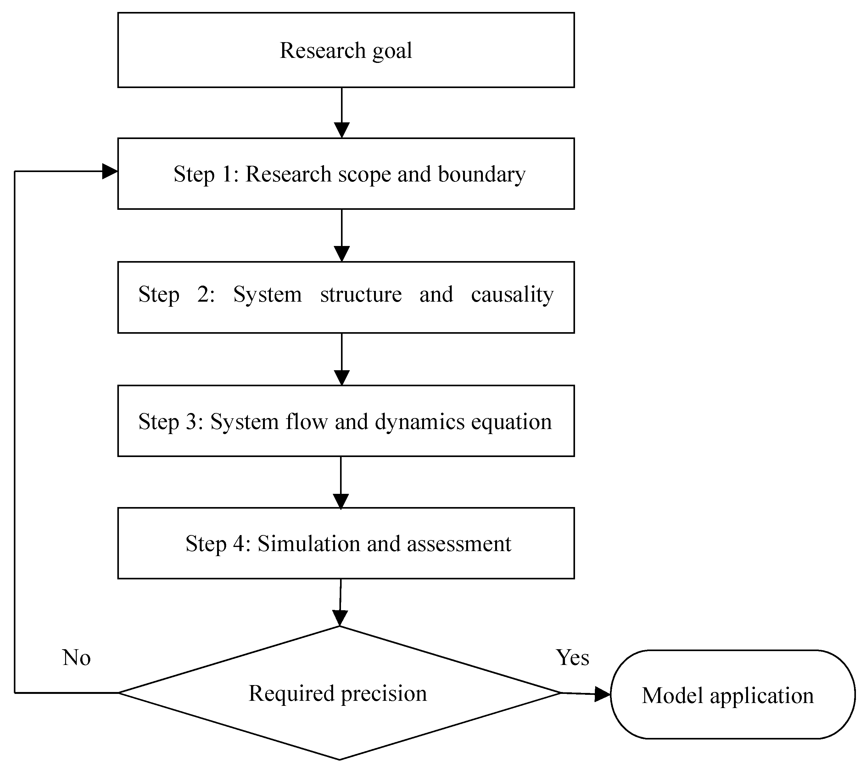
There are four steps for SD modeling process (Figure 1). The first step is to determine the research scope and boundary based on the research goal. In this step, the research object and boundary, as well as variables (the overview of parameters of private capital investment in public transport is listed in Table 1), are determined. The type, brief description, unit, and acronym used in the SD model are listed for each parameter. The following step is to divide the research object into sub-systems and determine their structures and causalities of variables (Figure 2). In Step 2, the causalities of variables and the relationships among sub-systems are analyzed. Then, the system flow diagram will be constructed to describe the positive or negative feedbacks among variables in the causality diagram. Based on the effect and cause relationships among variables, causal loops are determined [23]. At the same time, variable types are identified and classified, and dynamic equations are established to describe relationships among variables. The last step is SD model simulation and validation assessment. If the established SD model satisfies the required precision, the model can be used for variable analysis and policy-making; otherwise, it will return back to the first step and correct the model until it passes the required precision.
The system dynamic behavior simulation of private capital involvement in public transport starts with the constructions of sub-systems based on private capital investment strategies. According to the sub-system behavior characteristics of private capital investment strategies, the positive or negative feedback loops are formed for the supply and demand sub-systems which are directly related with the investment strategy sub-system. The lower-order sub-systems, together with the environmental transport sub-system, form the complicated simulation system of private capital involvement in public transport.
3. Passenger Value Investment Model in Public Transport
A recent paper by Xue [2,3] proposed a passenger value investment model in public transport. Passenger value has two meanings in public transport systems: for passengers, it means travel service supplied to passengers by public transport operators; and, in the other aspect, it means the benefits brought to public transport operators by passengers, including cash flow income of passengers’ public transport card balance, the fare income, and the ad revenue. Passengers of public transport form a very large customer base which can produce value besides ticket fares. The purpose of the passenger value investment model is to increase the public transport system welfare [2,3]. The welfares of the public transport system contain all the groups’ surpluses in public transport system. The surplus of the public transport company equals its benefits minus costs; the passengers’ surplus equals their respected fee minus the actual cost. It should be beneficial for passengers and public transport operators, as well as the public transport system, if the passenger value is well considered. There are two differences between the passenger value investment model and traditional investment model. One difference is that the cash flow profits in passengers’ public transport cards have changed from traditional bank interest to present investment profits. The investment profits rate is obviously higher than the rate of bank interest, because, in many developed countries (e.g., USA), there is no current interest and the current bank interest of a bank account is about 0.3–0.35% in China. Another difference is that the private sector may give part of the cash flow profits of the public transport cards to passengers. Then, it can reflect customer values of passengers and entice more people to travel by public transport.
A lease as one type of investment model is taken as an example, and it can be analyzed similarly for other investment models. Since the private sector is superior to public sector in the aspect of innovation, efficiency, technology advances, financial support, and competitions can provide benefits to the public transport system [4], it is reasonable to assume that a successful private capital involvement in public transport typically generates higher levels of efficiency compared with no private capital involvement. The public transport route is leased by the government to a private operator for a fee. In the lease contract, the private operator also shares the same financial subsidies from the government as the traditional public transport operators and takes on the operational risk fee. In the lease contract, passenger value and service quality constraints are considered, and it is permitted to utilize passenger resources as a customer base for the private operator and make use of cash flow in the passengers’ public transport cards accounts. To enhance competitive power and gain more profits, the private sector should improve the resource utilization efficiency; the above objective can be realized if private sectors make more efficient use of passenger resources. The proposed passenger value investment model could generate more profits, and should be more conducive for private capital investments in public transport.
4. Private Capital Investment SD Model in Public Transport
The transport environment sub-system, as well as the public transport demand and supply sub-systems, are selected as the research scope. The public transport sub-system contains the service level, potential public transport demand and benefits of the public transport company; the public transport supply sub-system contains profits of public transport, supply level (the amount of public transport vehicles), operational costs, and subsidies to public transport; and CO2, CO, SO2, PM10, and other motor vehicle emissions are included in the transport environment sub-system.
The research goal is to construct the private capital investment SD model in public transport, and to evaluate the advantages of the passenger value investment model from the aspect of the transport environment.
4.1. Private Capital Investment SD Model Construction in Public Transport
4.1.1. System Structure and Causalities of Private Capital Investments in Public Transport
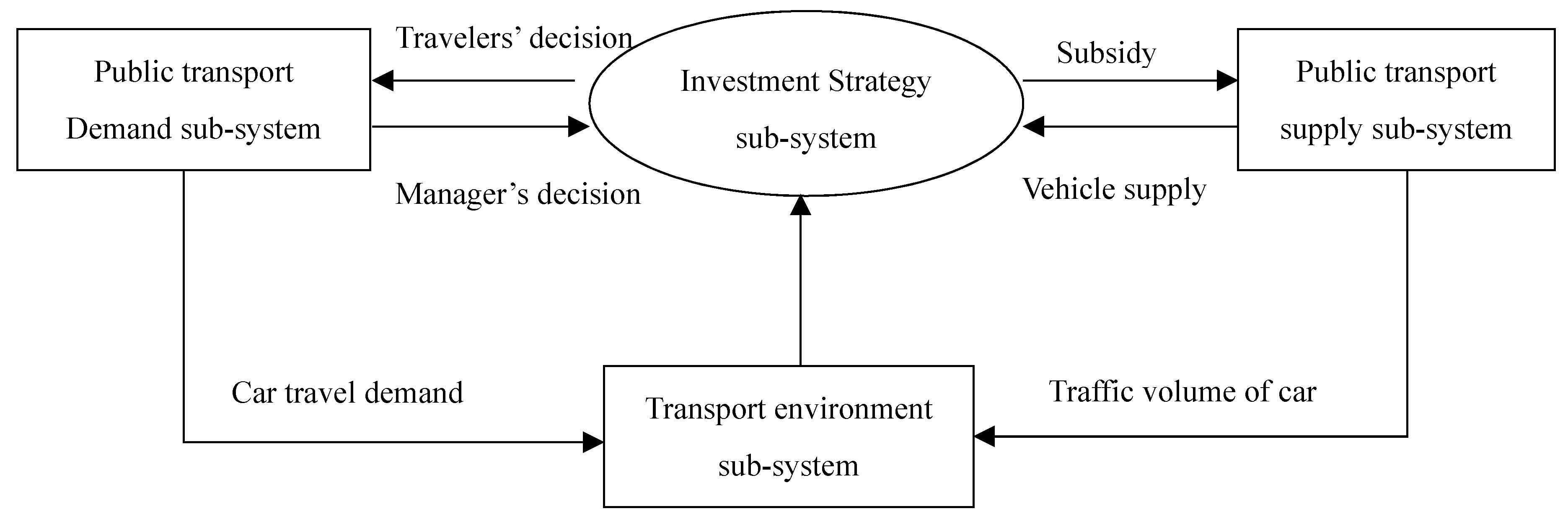
The simulation system structure of private capital investments in public transport means the causalities among variables in the public transport demand and supply sub-systems, strategy sub-system of private capital investment, and the transport environment sub-system. Figure 2 shows the system structure relationships of private capital investment in public transport, and the interactions among the four sub-systems. Private capital investment in public transport will affect travellers’ trip decisions. Compared to public sector, the private sector may make use of cash flows in passengers’ cards and give passengers some profits to attract more travellers to take public transport, passengers’ values can be reflected and more travellers will be enticed to take public transport; managers will adjust strategies for private capital investment according to public transport demand. Vehicle supply is the key variable in the public transport supply sub-system; the more profits and vehicle subsidies the operators have, the more public transport vehicles the operators can buy. The variations of public transport supply and demand can affect car travel demand, which indirectly affects the transport environment due to the different fuel consumption and emissions between public transport and private cars. The travel demands change and the different energy consumption and emissions between public transport and private cars lead to the changes in travel system energy consumption and emissions. The total emissions of public transport and private cars for a transport system in a period of time can be calculated based on system dynamic equations in the energy consumption and emission sub-system. Therefore, the transport environment sub-system has an environmental feedback to investment strategy sub-system. To better describe the environmental impacts of private capital investment, three sub-systems (investment strategy sub-system, public transport demand sub-system, and public transport supply sub-system) are considered to construct the private capital investment SD model in public transport. The environment sub-system is simulated only after the three sub-system SD model satisfies the model validation.
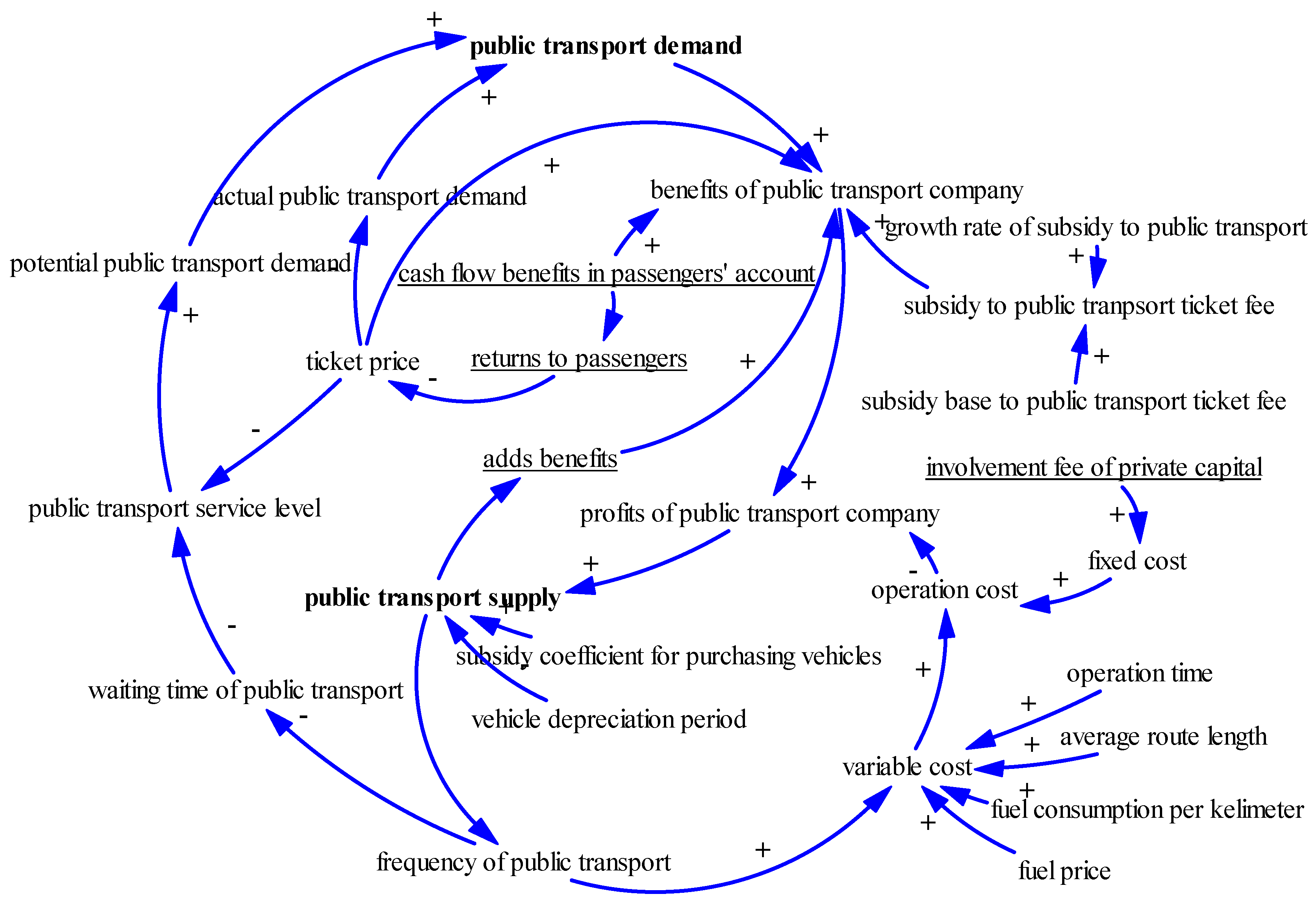
Figure 3 shows the causalities of passenger value private capital investment in public transport. The signs next to the arrows indicate the positive or negative correlations between variables. The underscored variables are the specific variables of private capital invests in public transport. Cash flow benefits in passengers’ account and returns to passengers are specific variables of the passenger value private capital investment model in public transport. The passenger value investment model [2,3] allows private capital to benefit from cash flow in passengers’ account via investment, which has a higher benefit ratio than bank interest. Since, in many developed countries (e.g., USA), there is no current interest and the current bank interest of a bank account is about 0.3–0.35% in China, the profit rate of successful investment is usually higher than 6% which is obviously higher than the rate of bank interest [2,3]. Private sectors return passengers some of the cash flow benefits to attract more travelers to travel by public transport. At the same time, the passenger value investment model increases benefits in the ads through constructing an e-commerce platform and advertising for business. The e-commerce platform and ads are closely related with the number of passengers, since, if the passenger value investment model can attract more travellers to travel by public transport, there will be more benefits in the e-commerce platform and ads business.
4.1.2. System Flow and Dynamic Equations of Private Capital Investments in Public Transport
Figure 4 shows the flow diagram of the passenger value private capital investment model in public transport. The major difference between Figure 3 and Figure 4 is that Figure 4 contains the input and output for level variables “potential public transport demand” and “public transport supply”. The variable values will change with time, and the changes are determined by dynamic equations. Figure 4 presents two flow and stock representations to illustrate the cumulative changes of public transport demand and supply. The links that are associated with each stock variable in Figure 4 are designated as rectangles [22]. Figure 3 just represents the causalities of variables without accumulative change process. However, Figure 4 focuses on the dynamic change process of system variables over time. There are inflows and outflows for key level variables listed in rectangles in Figure 4. Social network activities and personal reference generate different transport modes demand. The different traffic modes demand is also determined partially by switching among these traffic modes [22]. Only if the dynamic equations of variables in Figure 4 are established, the following numerical simulation can be conducted.
According to the variable roles in the system structure of private capital investment model in public transport, variables can be divided into four types as shown in Table 1: level variable, rate variable, auxiliary variable, and constant. Level variables are the variables that accumulate or decrease over time in a simulation system. Rate variables are the change rates of level variables in unit time. Auxiliary variables refer to intermediate process variables, equation parameter values, or input test functions. Constants are parameters that are not affected by changes in other variables.
This research is an extension of previous studies by Xue [2,3]. The previous studies all used the Jinan Public Traffic Company (Jinan city, Shandong Province, China) as an example; this paper also uses the same case for comparability and continuity. Table 2 gives the initial values of some parameters by taking Fleet 4 in No. 2 Company of the Jinan Public Traffic Company as an example. Other parameters are linked to the parameters in Table 2 via dynamic equations and determine the values. According to the existing research results by Sun [29], the public transport service level, which is an auxiliary variable and negatively related to public transport fare and waiting time, can be defined as the function of waiting time and public transport fare in the form of value of money in Equation (1):
where is the public transport ticket price; is the public transport waiting time; is the value of time of public transport passengers; a and b are the coefficients to be calibrated with the bus service data and public transport operation data [29]; and is the departure frequency of bus route i.
The dynamic equations in the SD model are divided into level models, rate models, auxiliary models, table functions, and constants. The capitalized first letter is used to denote the equation type in the following section. The dynamic equations of variable in Table 1 and Figure 4 are given according to the operation data of the Jinan Public Traffic Company [2,3].
L1: Potential public transport demand:
where J and K are time points; DT means time period from time J to time K; and is the attraction rate of the public transport service level.
L2: Public transport supply:
where mean the added vehicles and vehicle depreciation, respectively.
R1: Attraction rate of the public transport service level:
where R1 indicates the corresponding attraction rate of public transport under a certain service level. The lookup table function represents the correspondence relationship between the public transport service level and the public transport demand. The public transport demands under certain service levels are from historical data from the Jinan Public Traffic Company. KL means a period from time K to time L.
R2: Added public transport vehicles:
R3: Depreciation rate:
A1: Benefits of the public transport company:
A2: Subsidy to the public transport company:
A3: Profits of the public transport company:
A4: Departure frequency of public transport:
A5: Variable cost of the public transport company:
A6: Operational cost of the public transport company:
A7: Average waiting time:
A8: Service level of public transport:
A9: Deviation of the public transport service level:
A10: Cash flow benefits in passengers’ accounts:
where is the average amount of cash in passengers’ public transport cards. is the benefit rate of the cash flow in passengers’ public transport cards.
A11: Returns to passengers:
where is the return rate to passengers, meaning the ratio of returns to passengers over cash flow benefits in passengers’ accounts. takes the value 0.5 in the case study, but it can also take other values. We can analyze the effects of under different values and find an optimization value for .
A12: Ad benefits:
A13: Actual public transport demand:
Actual public transport demand is represented through a lookup function. This means the detailed public transport demands under different public transport ticket prices. The specific values can be gained from the Jinan Public Traffic Company and the Public Transport Logit Model of Jinan City [2]. N equations (constant) can be seen in Table 3.
4.2. SD Model Simulation and Validation
Due to different variables or different model structures, the model simulation results may be different. Therefore, SD model validation is needed before model simulation to realize the consistent relationship between established private capital investment SD model in public transport and the Jinan City public transport structure. Based on the commonly-used statistical theory, a 95% confidence level is recognized as an objective criterion. Therefore, if the reliability level is used as a test standard, the prediction error of SD model should be within ±5% to meet the accuracy requirements [29]. Sun [29] chose two level variables (public transport demand and public transport vehicles) to test the SD model of the public transport price linkage strategy. In this paper, two level variables, public transport demand (trip/month) and public transport supply (public transport vehicles), are chosen as test variables. The established SD model above is used to simulate passenger volume and operation vehicles in Fleet 4, No. 2 Company of the Jinan Public Traffic Company in 2011. Then the simulation results will be compared with the statistical data. Table 3 shows that the relative errors of the two test indicators are within ±5%, the established private capital investment SD model in public transport satisfies accuracy requirements. The SD model simulation experience is effective and it can be used to analyze the impacts of private capital investment on the environmental sub-system in public transport system. The SD model simulation and validation just show the constructed SD model in the manuscript is suitable to simulate Fleet 4, No. 2 Company of the Jinan Public Traffic Company. If the model is applied in another context, perhaps the SD model structure and system parameters are similar, but the calibrated coefficients of variables in the system dynamic equations may be different. However, the SD model established in the paper may have the same model structure as the model in another context. From this point of view, the SD model structure can be applied in another context.
5. Case Study
5.1. Case Introduction
Jinan City, which is the capital of Shandong Province, China, was selected as the case study. Based on the author’ previous research [3], the passenger value private capital investment model in public transport is evolutionarily stable, which means all the operators will adopt the passenger value investment model. The previous research [3] also takes Jinan City as an example, the research background and the analysis data are similar with this paper. Therefore, it is reasonable that the research results in [3] are also valid in this case. In the following subsections, three simulation environments will be compared with each other to see whether the passenger value investment model is still superior from the environmental point of view. The three simulation environments are, respectively, the present travel environment, the traditional private capital investment and passenger value investment travel environments. According to the Jinan residents travel survey [2,3] in 2011 (Table 4), the operation date of 100 public transport vehicles in Fleet 4 of the No. 2 company of the Jinan Public Traffic Company is chosen as the simulation data. Since the residents’ travel survey in 2011 is official and is the largest-scale travel survey in Jinan City, it is authoritative and representative. Other parameters can be seen in Table 1. To study the SD evaluation model, Jinan City is taken as an example to collect the basic data, including residents’ travel data, public transport operation data, and financial data. The comprehensive traffic survey, which is carried out regularly and irregularly at home and abroad in large- and medium-sized cities, provides a data source for residents’ travel data. At the same time, more extensive data can be obtained via the information method. It is not a problem for government departments to encourage private capital investment to collect public transport data. The feasibility of data acquisition provides data support for the SD model construction and impacts the evaluation of private capital invests in public transport, and also improves the portability of the quantitative SD model. Therefore, it is possible for public sectors to have all the required data available for the simulation.
Figure 5 describes the variables and their relationships in the public transport environmental sub-system. The travel demands change and the different energy consumption and emissions between public transport and private cars lead to the changes in travel system energy consumption and emissions. The total emissions of public transport and private cars in the cumulative 100 months can be calculated based on Figure 5. Equations (20)–(27) are mathematical expressions of the system dynamic equations in the energy consumption and emission sub-system:
where is initial public transport demand; is the initial public transport supply; is average car carrying capacity, which equals 1.5 persons/car; L is the average mileage; is the emission factor [29] (Table 5); is the emission change of vehicles; is the average fuel consumption unit mileage (see Table 2 and Table 4); and is the fuel consumption change of vehicles in the transport system.
5.2. Simulation Results and Environmental Impact Analyses
Figure 6 shows the cumulative change processes of public transport demand and supply in the case under three comparable conditions [2,3], which are whether or not to give passengers some returns, and without and with private capital investment. Based on the research results in [2,3], investment with returns is superior to traditional investment, and traditional investment is superior to the condition without private capital investment in public transport. The public transport demand and supply curves under the traditional investment condition lie between the curves under the other two conditions (Figure 6). As seen in Figure 6, public transport demand and supply also increase cumulatively under the three conditions. Since the passenger value investment model gains more profits and gives some returns to passengers, its public transport demand and supply increase most rapidly. According to Equations (2)–(9), the changes of travel demands and supplies, as well as the different energy consumption and emissions between public transport and private cars lead to the system changes of energy consumption and emissions. Figure 7 also shows that the cumulative trend of transport system energy consumption and emissions is consistent with the trend of public transport demand and supply.
Figure 7 gives the cumulative emission reductions during 100 months under the traditional investment model and investment with returns compared with no private capital investment. From the perspective of environmental protection, the contract period of private capital investing in public transport should not be short, but long, because the cumulative reduced emissions are exponential. As seen in Figure 7c, it is effective after 50 months for SO2 reduction and the cumulative reduction amount of SO2 is negative before 50 months because private cars have very low SO2 emission factor compared with public transport (as seen in Table 5). It will have a positive effect on SO2 emission reductions if the contact period of private capital investment in public transport is longer than four years in the case. Figure 7 shows that, in a cumulative period of 100 months, the passenger value investment model in the case, respectively, reduces emissions of CO2, CO, SO2, and PM10 by 109 tons, 542 kg, 1.6 kg, and 77.3 kg compared with no private capital investment. Meanwhile the emission reductions of CO2, CO, SO2, and PM10 are, respectively, 69 tons, 339 kg, 1.1 kg, and 48 kg compared with the traditional investment model. It is obvious to calculate other emission reductions based on the corresponding emission factors.
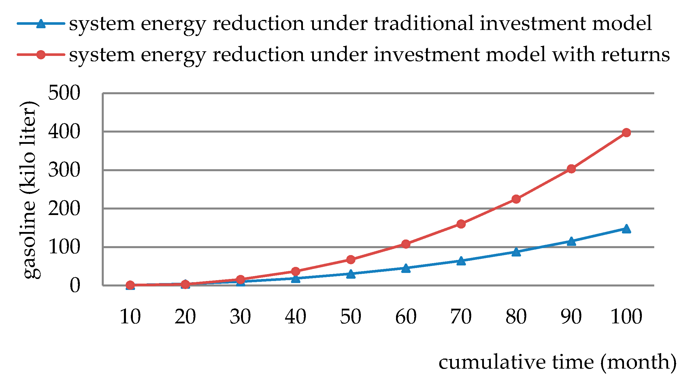
Figure 8 shows the energy-saving effect of the investment model with returns and the traditional investment model compared with no private capital investment. The cumulative trends of system energy reductions in Figure 8 are consistent with the change trends of public transport demand and supply in Figure 6. The cumulative energy reductions of the two investment models compared with no private capital investment are, respectively, 398 kiloliters and 148 kiloliters. There are 250 kiloliters more energy savings for the investment model with returns than the traditional investment model.
To sum up, there are considerable cumulative emission reductions and energy-savings for the investment model with returns and the traditional investment model compared with no private capital investment. Although the relative value of emission reduction for private capital investment model is small (the value is 0.58%, and it equals the emission reduction value under private capital investment divided by the total emission value without private capital investment), the cumulative absolute value of emission reductions is obvious. Since the case is only for one public transport fleet and there are 40 fleets in Jinan City, the cumulative energy-savings and emission reductions are very impressive from the whole city’s point of view. The case results show that, from the environmental point of view, private capital investment in public transport with returns to passengers (passenger value investment model) is superior to the traditional investment model and no private capital investment. Therefore, the investment model considering passenger value should be encouraged from the aspect of environmental protection.
6. Conclusions
The SD method is used in the paper to analyze the cumulative effect of private capital investment in public transport from the perspective of the environment. A private capital investment SD simulation model is constructed and validated based on the Jinan Public Traffic Company. The simulation results show that the passenger value private capital investment model in public transport has a more significant cumulative effect of energy-saving and emission reductions. The passenger value investment model is verified to be superior from the perspective of the environment. The established SD model provides a theoretical tool for the managers to quantitatively evaluate the effects of energy-savings and emission reductions of private capital invests in public transport.
Frankly speaking, there are also shortcomings in the research and deeper study should be developed in the future. (i) Only the local fleet is selected for analysis at present as a result of the simplified processing of the scenario settings; thus, the scope of the study can be expanded in the following study. (ii) The SD model constructed in the paper contains a number of variables that are settled to the effect of energy-savings and emission reductions; thus, the cumulative effect of causal interactions between variables can also be further analyzed. (iii) In the simulation period of 100 months, vehicle upgrading problem and other changeable conditions are not considered. The decline in fuel consumption and the possible increase in emissions standards are more in accordance with the reality. Another problem may be that the private company could do so well that they try to renegotiate the subsidy (or the contract) with the public administration, and this would make the results inefficient (since the cost-efficiency of one dollar invested is now changed due to this circumstance). On the other hand, in that period, some large cities could be experiencing a boom in public transportation demand, which could be useful for the application of the paper. Additionally, the PPP may be profitable only if the contract lasted for a certain number of years, which should be compared to the optimal length of the contract to introduce competition in the market. This fact could affect the incentives of the private companies to be more efficient and competitive. However, this will significantly increase the complexity of the SD model and the simulation solution difficulty, which is worthy of deeper analysis in future research.
Acknowledgments
This research was sponsored by the National Natural Science Foundation of China (grant Nos. 51338008, 51378036, 51308015, 51308016, and 51308018); the Jiangxi Province Natural Science Foundation Management Science Project (grant no. 708258897028); the Key Research and Development Program of Jiangxi Province (grant No. 20161BBG70080); the Doctoral Research Foundation of East China Jiao Tong University (grant No. 2003417029); the Nanning Key Research Project of Qinghai Province of China (grant No. 2015-SF-A5); and the Beijing National Science Foundation (grant No. 8163045). The authors give thanks to Jinan Public Traffic Company for operational data. The authors are also grateful for the editor’s and the anonymous reviewers’ comments and time.
Author Contributions
The individual responsibilities and contribution of the authors are listed as follows: Yunqiang Xue designed the research, collected and analyzed the data, developed the model and conducted the model validation, and wrote the paper; Hongzhi Guan guided the research process; Jonathan Corey revised the manuscript, provided some comments, and helped edit the manuscript; Bing Zhang edited the manuscript and gave some comments on the case study; Hai Yan gave some comments and edited the manuscript; Yan Han gave some comments on the SD model and improved the model; and Huanmei Qin provided some comments on case study and edited the manuscript.
Conflicts of Interest
The authors declare no conflict of interest.
References
- Malandraki, G.; Papamichail, I.; Papageorgiou, M.; Dinopoulou, V. Simulation and Evaluation of a Public Transport Priority Methodology. Transp. Res. Procedia 2015, 6, 402–410. [Google Scholar] [CrossRef]
- Xue, Y.; Guan, H.; Correy, J.; Qin, H.; Han, Y.; Ma, J. Bilevel Programming Model of Private Capital Investment in Urban Public Transportation: Case Study of Jinan City. Math. Probl. Eng. 2015, 2015, 498121. [Google Scholar] [CrossRef]
- Xue, Y.; Guan, H.; Corey, J.; Wei, H.; Yan, H. Quantifying a Financially Sustainable Strategy of Public Transport: Private Capital Investment Considering Passenger Value. Sustainability 2017, 9, 269. [Google Scholar] [CrossRef]
- Chan, A.P.C.; Lam, P.T.I.; Chan, D.W.M.; Cheung, E.; Ke, Y. Privileges and attractions for private sector involvement in PPP projects. In Challenges, Opportunities and Solutions in Structural Engineering and Construction-Ghafooi; Ghafoori, N., Ed.; Taylor & Francis Group: London, UK, 2010; pp. 751–755. [Google Scholar]
- Costa, A.; Fernandes, R. Urban public transport in Europe: Technology diffusion and market organization. Transp. Res. Part A 2012, 46, 269–284. [Google Scholar] [CrossRef]
- Matsunaka, R.; Oba, T.; Nakagawa, D.; Nagao, M.; Nawrocki, J. Internatioal comparison of the relationship between urban structure and the service level of urban public transportation—A comprehensive analysis in local cities in Japan, France and Germany. Transp. Policy 2013, 30, 26–39. [Google Scholar] [CrossRef] [Green Version]
- Medda, F.R.; Carbonaro, G.; Davis, S.L. Public private partnerships in transportation: Some insights from the European experience. IATSS Res. 2013, 36, 83–87. [Google Scholar] [CrossRef]
- Osei-Kyei, R.; Chan, A.P.C. Review of studies on the Critical Success Factors for Public-Private Partnership (PPP) projects from 1990 to 2013. Int. J. Proj. Manag. 2015, 33, 1335–1346. [Google Scholar] [CrossRef]
- English, L.M. Public Private Partnerships in Australia: An Overview of Their Nature, Purpose, Incidence and Oversight. UMSW Law J. 2006, 29, 250–263. [Google Scholar]
- Group, W.B. Public-Private Partnerships Reference Guide-Version 2.0; World Bank: Washington, DC, USA, 2014. [Google Scholar]
- Rouhani, O.M.; Niemeier, D. Resolving the property right of transportation emissions through public-private partnerships. Transp. Res. Part D Transp. Environ. 2014, 31, 48–60. [Google Scholar] [CrossRef]
- De Los Rios-Carmenado, I.; Ortuno, M.; Rivera, M. Private-Public Partnership as a Tool to Promote Entrepreneurship for Sustainable Development: WWP Torrearte Experience. Sustainability 2016, 8, 199. [Google Scholar] [CrossRef]
- Bidne, D.; Kirby, A.; Luvela, L.J.; Shattuck, B.; Standley, S.; Welker, S. The Value for Money Analysis: A Guide for More Effective PSC and PPP Evaluation. Available online: http://www.ncppp.org/wp-content/uploads/2013/03/PS-051012ValueForMoney-paper.pdf (accessed on 26 September 2017).
- Takim, R.; Ismail, K.; Nawawi, A.H.; Jaafar, A. The Malaysian Private Finance Initiative and Value for Money. Asian Soc. Sci. 2009, 5, 103–111. [Google Scholar] [CrossRef]
- Ho, P.H.K. Development of Public Private Partnerships (PPPs) in China. Available online: http://www.icoste.org/Roundup1206/HoPaper.pdf (accessed on 26 September 2017).
- Zhang, S.; Chan A P, C.; Feng, Y.; Duan, H.; Ke, Y. Critical review on PPP Research—A search from the Chinese and International Journals. Int. J. Proj. Manag. 2016, 34, 597–612. [Google Scholar] [CrossRef]
- Mounter, N.; Annema J, A.; van Wee, B. Managing the insolvable limitations of cost-benefit analysis: Results of an interview based study. Transportation 2015, 42, 277–302. [Google Scholar] [CrossRef]
- Soomro, M.A.; Zhang, X. Value for Money Drivers in Transportation Public Private Partnerships. In Proceedings of the 24th International Project Management Association (IMPA) World Congress, Istanbul, Turkey, 1–3 November 2010. [Google Scholar]
- Morallos, D.; Amekudzi, A. A Review of Value-for-Money Analysis for Comparing Public-Private Partnerships with Traditional Procurements. In Proceedings of the Transportation Research Board 87th Annnual Meeting, Washington, DC, USA, 13–17 January 2008. [Google Scholar]
- Peng, W.; Cui, Q.; Lu, Y.; Huang, L. Achieving Value for Money: An Analytic Review of Studies on Public Private Partnerships. In Proceedings of the Construction Research Congress 2014, Atlanta, GA, USA, 19–21 May 2014. [Google Scholar]
- Miller, P.; de Barros, A.G.; Kattan, L.; Wirasinghe, S.C. Public Transportation and Sustainability: A Review. KSCE J. Civ. Eng. 2016, 20, 1076–1083. [Google Scholar] [CrossRef]
- Liu, S.; Triantis, K.P.; Sarangi, S. A framework for evaluating the dynamic impacts of a congestion pricing policy for a transportation socioeconomic system. Transp. Res. Part A Policy Pract. 2010, 44, 596–608. [Google Scholar] [CrossRef]
- Egimez, G.; Tatari, O. A dynamic modelling approach to highway sustainability: Srategies to reduce overall impact. Transp. Res. Part A 2012, 46, 1086–1096. [Google Scholar]
- Sterman, J. System dynamics modeling: Tools for learning in a complex world. Calif. Manag. Rev. 2001, 43, 8–25. [Google Scholar] [CrossRef]
- Forrester, J.W. 479 Industrial Dynamics; Wiley-Interscience: New York, NY, USA, 1961. [Google Scholar]
- Wang, J.; Lu, H.; Peng, H. System dynamics model of urban transportation system and its application. J. Transp. Syst. Eng. Inf. Technol. 2008, 8, 83–89. [Google Scholar] [CrossRef]
- Fong, W.; Matsumoto, H.; Lun, Y. Application of system dynamics model as decision making tool in urban planning process toward stabilizing carbon dioxide emissions from cities. Build. Environ. 2009, 44, 1528–1537. [Google Scholar] [CrossRef]
- Baldoni, F.; Falsini, D.; Taibi, E. A system dynamics energy model for a sustainable transportation system. In Proceedings of the 28th International Conference of the System Dynamics Society, Seoul, Korea, 25–29 July 2010. [Google Scholar]
- Guanglin, S. Research on Price Linkage Strategy of Public Transport of City. Ph.D. Thesis, Harbin Institute of Technology, Harbin, China, 2013. (In Chinese). [Google Scholar]
Figure 1.
Modeling process of system dynamics.

Figure 2.
Private capital investment system structure in public transport.

Figure 3.
System causalities of passenger value private capital investment model in public transport.
Figure 3.
System causalities of passenger value private capital investment model in public transport.

Figure 4.
System flow of passenger value private capital investment model in public transport.

Figure 5.
Relationships of the variables in the environmental sub-system of public transport system.
Figure 5.
Relationships of the variables in the environmental sub-system of public transport system.
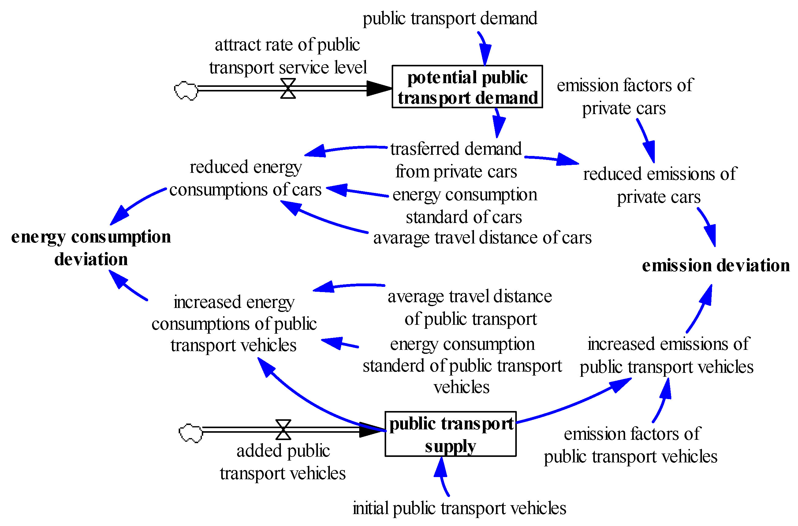
Figure 6.
The variation process of: (a) public transport supply; and (b) demand under different investment models.
Figure 6.
The variation process of: (a) public transport supply; and (b) demand under different investment models.
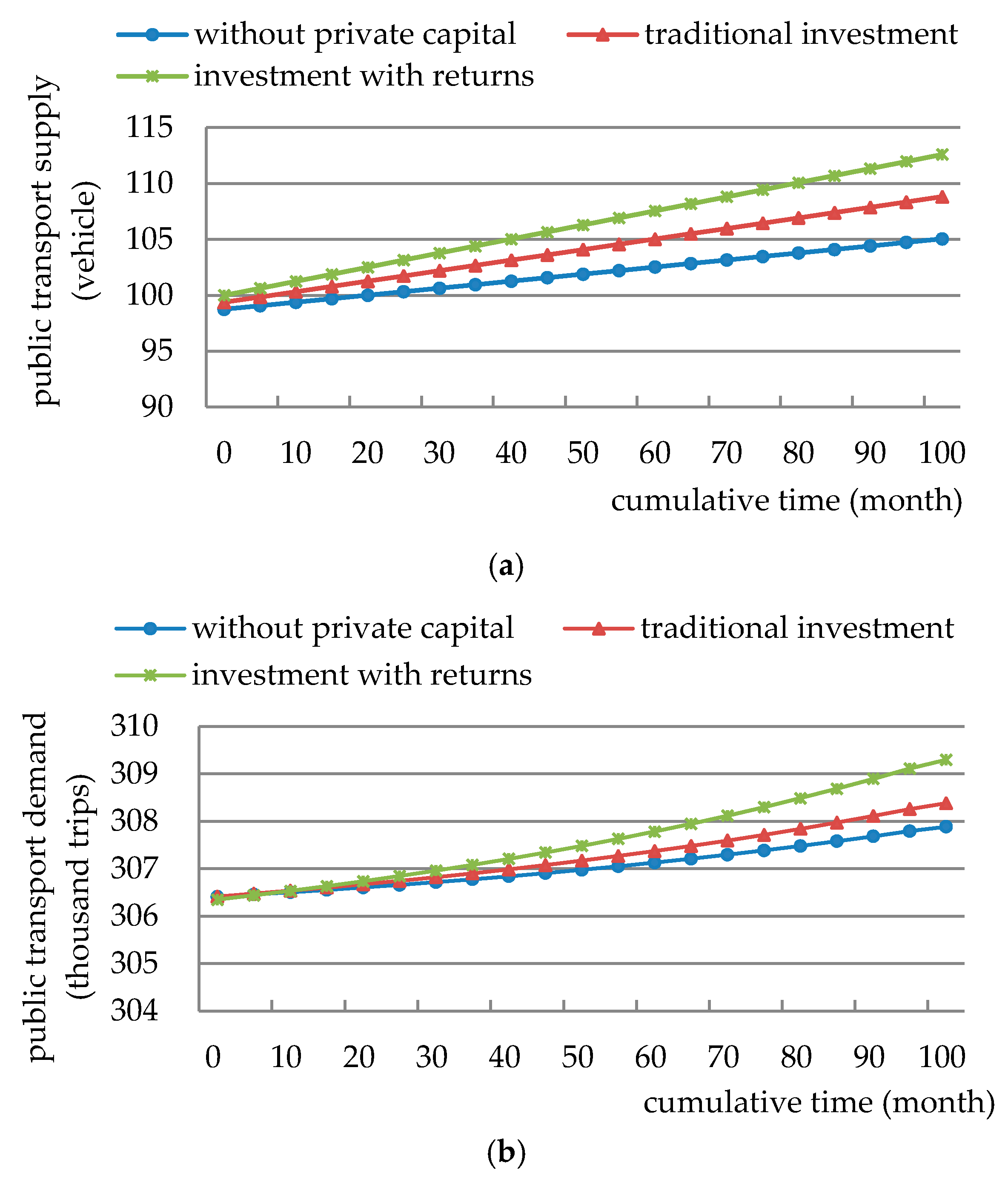
Figure 7.
Reduction emissions of: (a) CO2; (b) CO; (c) SO2; and (d) PM10 under different investment models.
Figure 7.
Reduction emissions of: (a) CO2; (b) CO; (c) SO2; and (d) PM10 under different investment models.
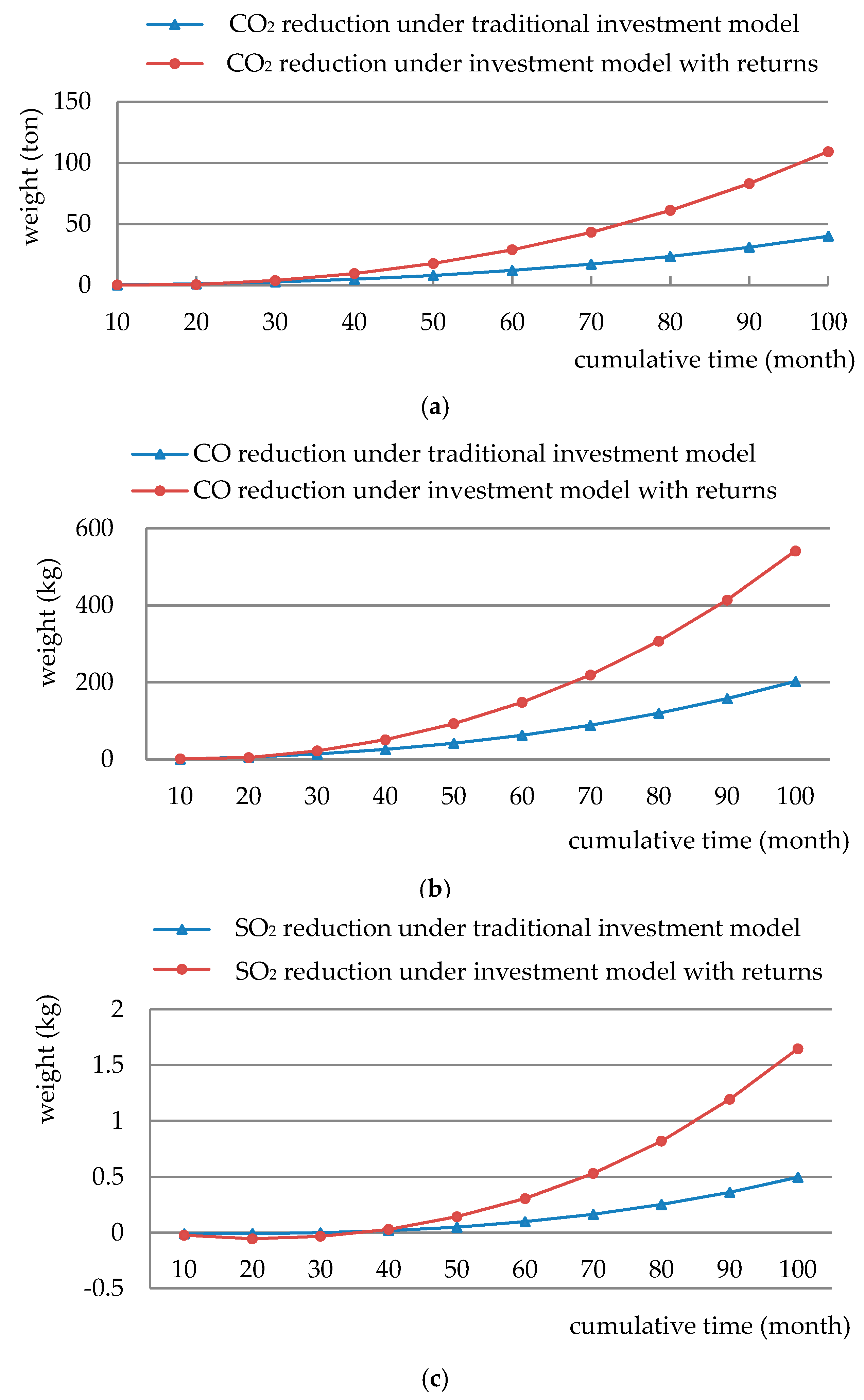
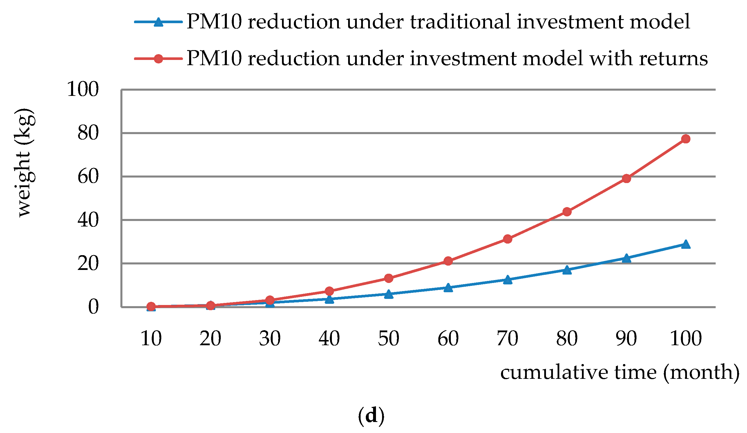
Figure 8.
Reduction of energy consumption under different investment models.


Table 1.
System parameters of private capital investment in public transport.
| Variable Type | Variable | Unit | Symbol | Illustration |
|---|---|---|---|---|
| Level variable | Public transport supply | vehicle | Operation vehicles of public transport | |
| Potential demand | trip | Transfer amount from other travel mode | ||
| Public transport demand | trip | Actual and potential public transport demand | ||
| Rate variable | Attract rate of public transport service level | Public transport demand at different service levels; it presents the fitting slope between public transport demand and service levels | ||
| Vehicle depreciation rate | The ratio of depreciation value to total vehicle value | |||
| Added vehicles | vehicle | The added public transport vehicles per year | ||
| Auxiliary variable | Benefits of public transport company | Yuan | Sum of fare income, ad income, subsidies, and cash flow benefits in passengers’ accounts | |
| subsidy | Yuan | Government subsidy to public transport | ||
| Profits of public transport company | Yuan | Benefits of public transport company minus cost | ||
| Departure frequency | Bus/hour | Departure frequency of public transport | ||
| Variable cost | Yuan | Related to operation time, route length, fuel consumption and fuel price | ||
| Operation cost | Yuan | Variable cost plus fixed cost | ||
| Waiting time | hour | Average waiting time of public transport | ||
| Service level | A function of ticket price and travel time of public transport [29] | |||
| Difference of service levels | Difference between actual and respected public transport service levels | |||
| Benefits of cash flow in passengers’ accounts | Yuan | Benefits of cash flow in passengers’ account through investment in other fields | ||
| Returns to passengers | Yuan | Some of cash flow benefits returned to passengers | ||
| Adds benefits | Yuan | Adds benefits of public transport | ||
| Actual public transport demand | trip | Actual travel demand of public transport | ||
| constant | Subsidy base | Yuan | Original subsidy amount to public transport | |
| Subsidy growth rate | Growth rate of subsidy to public transport ticket fee | |||
| Subsidy coefficient of vehicle purchase | Ratio of subsidy to total vehicle price | |||
| Involvement fee | Yuan/day | Involvement fee of private capital | ||
| Time value of passengers | Yuan/hour | Related to passengers’ average income per hour | ||
| Fixed operation cost | Yuan | Fixed operation cost of public transport | ||
| Respected service level | The service level passengers respect | |||
| Public transport route length | km | Average route length of public transport | ||
| Fuel consumption of public transport | Liter/Km | Average fuel consumption of public transport | ||
| Fuel price 1 () | Yuan/liter | Market price minus fuel subsidy |
1 To simplify the calculation process, fuel price is treated as a constant. In fact, it is reasonable, since the government will subsidize public transport operators so that operators can pay less on fuel. Although the market fuel price is fluctuating, the government can maintain the final fuel price for public transport operators at a stable level via fluctuating the fuel subsidy.
Table 2.
Initial values of parameters in SD model.
| Variable | Initial Value |
|---|---|
| Potential public transport demand | 0 |
| Public transport supply | 100 vehicles |
| Subsidy base to public transport ticket fee | 10,000 Yuan |
| Growth rate of subsidy to public transport | 1% |
| Time value of public transport passengers | 30 Yuan/h |
| Fixed operation cost | 20,000 Yuan/month |
| Subsidy coefficient for purchasing vehicles | 0.6% |
| Fuel price | 6 Yuan/L |
| Average route length | 15 km |
| Fuel consumption per kilometer for public transport vehicles | 0.3 L/km |
| Respected public transport service level | 4 |
| Average operation time of public transport | 360 h/month/vehicle |
Table 3.
SD model validation.
| Validation Parameter (Level Variable) | Simulation Results | Statistic Results | Relative Error |
|---|---|---|---|
| Public transport demand (trip/month) | 306,450 | 322,000 | –4.83% |
| Public transport supply (vehicles amount) | 97 | 100 | –3% |
Table 4.
Travel indicators of public transport and private car of Jinan City.
| Parameter | Survey Value | Parameter | Survey Value |
|---|---|---|---|
| Car travel demand | 1.80 million trips/day | Public transport demand | 2.40 million trips/day |
| Average car carrying capacity | 1.5 persons/vehicle | Average passenger capacity | 70 persons/vehicle |
| Average travel mileage of car | 10.6 km | Average travel mileage of public transport | 11 km |
| Average speed of private car | 21 km/h | Average speed of public transport | 17 km/h |
| Average fuel consumption of private car | 0.07 L/km |
Table 5.
Major emission factors of car and public transport [29].
Table 5.
Major emission factors of car and public transport [29].
| Vehicle Type | Fuel Type | Emission Standards | Emission Factor (g/km) | |||
|---|---|---|---|---|---|---|
| CO2 | CO | SO2 | PM10 | |||
| Car | Gasoline | Euro IV | 322.3 | 1.4 | 0.01 | 0.2 |
| Euro V | 322.3 | 1.4 | 0.01 | 0.2 | ||
| Bus | Gasoline | Euro IV | 1072.8 | 0.3 | 0.30 | 0.1 |
| Euro V | 1072.8 | 0.3 | 0.30 | 0.1 | ||
| CNG | Euro III | 1254.8 | 1.0 | 0.00 | 0.1 | |
© 2017 by the authors. Licensee MDPI, Basel, Switzerland. This article is an open access article distributed under the terms and conditions of the Creative Commons Attribution (CC BY) license (http://creativecommons.org/licenses/by/4.0/).
Share and Cite
MDPI and ACS Style
Xue, Y.; Guan, H.; Corey, J.; Zhang, B.; Yan, H.; Han, Y.; Qin, H. Transport Emissions and Energy Consumption Impacts of Private Capital Investment in Public Transport. Sustainability 2017, 9, 1760. https://doi.org/10.3390/su9101760
AMA Style
Xue Y, Guan H, Corey J, Zhang B, Yan H, Han Y, Qin H. Transport Emissions and Energy Consumption Impacts of Private Capital Investment in Public Transport. Sustainability. 2017; 9(10):1760. https://doi.org/10.3390/su9101760
Chicago/Turabian StyleXue, Yunqiang, Hongzhi Guan, Jonathan Corey, Bing Zhang, Hai Yan, Yan Han, and Huanmei Qin. 2017. "Transport Emissions and Energy Consumption Impacts of Private Capital Investment in Public Transport" Sustainability 9, no. 10: 1760. https://doi.org/10.3390/su9101760
Note that from the first issue of 2016, this journal uses article numbers instead of page numbers. See further details here.