Risk Measurement and Risk Modelling Using Applications of Vine Copulas


1
School of Mathenatics and Statistics, Sydney University, Sydney, NSW 2006, Australia
2
School of Business and Law, Edith Cowan University, Joondalup, WA 6027, Australia
3
Department of Quantitative Finance, National Tsing Hua University, 30013 Hsinchu City, Taiwan
4
Discipline of Business Analytics, University of Sydney Business School, Sydney, NSW 2006, Australia
5
Econometric Institute, Erasmus School of Economics, Erasmus University Rotterdam, 3062 PA Rotterdam, The Netherlands
6
Department of Quantitative Economics, Complutense University of Madrid, 28040 Madrid, Spain
7
Institute of Advanced Sciences, Yokohama National University, 240-8501 Yokohama, Japan
*
Author to whom correspondence should be addressed.
Sustainability 2017, 9(10), 1762; https://doi.org/10.3390/su9101762
Submission received: 8 August 2017
/
Revised: 10 September 2017
/
Accepted: 13 September 2017
/
Published: 29 September 2017
(This article belongs to the Special Issue Risk Measures with Applications in Finance and Economics)
Abstract
:This paper features an application of Regular Vine copulas which are a novel and recently developed statistical and mathematical tool which can be applied in the assessment of composite financial risk. Copula-based dependence modelling is a popular tool in financial applications, but is usually applied to pairs of securities. By contrast, Vine copulas provide greater flexibility and permit the modelling of complex dependency patterns using the rich variety of bivariate copulas which may be arranged and analysed in a tree structure to explore multiple dependencies. The paper features the use of Regular Vine copulas in an analysis of the co-dependencies of 10 major European Stock Markets, as represented by individual market indices and the composite STOXX 50 index. The sample runs from 2005 to the end of 2013 to permit an exploration of how correlations change indifferent economic circumstances using three different sample periods: pre-GFC (January 2005–July 2007), GFC (July 2007– September 2009), and post-GFC periods (September 2009–December 2013). The empirical results suggest that the dependencies change in a complex manner, and are subject to change in different economic circumstances. One of the attractions of this approach to risk modelling is the flexibility in the choice of distributions used to model co-dependencies. The practical application of Regular Vine metrics is demonstrated via an example of the calculation of the VaR of a portfolio made up of the indices.
1. Introduction
In the last decade copula modelling has become a frequently used tool in financial economics. Accounts of copula theory are available in [1,2]. Hierarchical, copula-based structures have recently been used in some new developments in multivariate modelling; notable among these structures is the pair-copula construction (PCC). Joe (1996) [3] originally proposed the PCC and further exploration of its properties has been undertaken by Bedford and Cooke [4,5] and Kurowicka and Cooke (2006) [6]. Aas et al., (2009) [7] provided key inferential insights which have stimulated the use of the PCC in various applications, (see, for example, Schirmacher and Schirmacher (2008) [8], Chollete et al. [9], Heinen and Valdesogo [10], Berg and Aas [11], Min and Czado [12] and Smith et al. [13]. Allen et al., (2013) [14] provide an illustration of the use of R-Vine copulas in the modelling of the dependences amongst Dow Jones Industrial Average component stocks, and this study is a companion piece.
There have also been some recent applications of copulas in the context of time series models (see the survey by Patton (2009) [15], and the recently developed COPAR model of Breckmann and Czado [16], which provides a vector autoregressive VAR model for analysing the non-linear and asymmetric co-dependencies between two series). Nevertheless, in this paper we focus on static modelling of dependencies based on R Vines in the context of modelling the co-dependencies of ten major European markets as captured by ten major indices and one composite European index. We use the British market represented by the FTSE100, the German market as captured by the DAX, the French market via the CAC40, the Netherlands, via the AEX index, the Spanish market represented by the IBEX35, the Danish market by means of the OMX Copenhagen 20, the Swedish market represented by the OMX Stockholm PI Index, the Finnish market using the OMXHPI, the Portuguese market using the PSI General Index (BVLG) and the Belgian market via the Belgian market via the Bell 20 Index (BFX). We also use the EURO STOXX 50 Index, Europe’s leading Blue-chip index for the Eurozone, which consists of 50 major stocks from 12 Eurozone countries: Austria, Belgium, Finland, France, Germany, Greece, Ireland, Italy, Luxembourg, The Netherlands, Portugal and Spain. We undertake our analysis in three different sample periods which include the GFC; pre-GFC (Jan 2005–July 2007), GFC (July 2007–September 2009), and post-GFC periods (September 2009–December 2013). To further show the capabilities of this flexible modelling technique, we also use R-Vine Copulas to quantify Value at Risk for an equally weighted portfolio of our eleven European indices, as an empirical example. The main aim of the paper is to demonstrate the useful application of both C-Vine and R-Vine measures of co-dependency at at time of extreme financial stress and its effectiveness in teasing out changes in co-dependency.
The paper is divided into five sections: the next section provides a review of the background theory and models applied, Section 3 introduces the sample, Section 4 and Section 5 present the results for our analyses featuring C-Vine and R-Vines, Section 6 provides an example of the use of R-Vines to forecast the Value-at-Risk (VaR) and a brief conclusion follows in Section 7.
2. Background and Models
Sklar (1959) [17] provides the basic theorem describing the role of copulas for describing dependence in statistics, providing the link between multivariate distribution functions and their univariate margins. We can speak generally of the copula of continuous random variables . The problem in practical applications is the identification of the appropriate copula.
Standard multivariate copulas, such as the multivariate Gaussian or Student-t, as well as exchangeable Archimedean copulas, lack the exibility of accurately modelling the dependence among larger numbers of variables. Generalizations of these offer some improvement, but typically become rather intricate in their structure, and hence exhibit other limitations such as parameter restrictions. Vine copulas do not suffer from any of these problems.
Initially proposed by Joe [3] and developed in greater detail in Bedford and Cooke [4,5] and in Kurowicka and Cooke [6], vines are a flexible graphical model for describing multivariate copulas built up using a cascade of bivariate copulas, so-called pair-copulas. Their statistical breakthrough was due to Aas, Czado, Frigessi, and Bakken [7] who described statistical inference techniques for the two classes of canonical C-vines and D-vines. These belong to a general class of Regular Vines, or R-vines which can be depicted in a graphical theoretic model to determine which pairs are included in a pair-copula decomposition. Therefore a vine is a graphical tool for labelling constraints in high-dimensional distributions.
This area of the literature has expanded rapidly. Joe et al., (2010) [18] explore the tail dependence and conditional tail dependence functions of vine copulas of lower-dimensional margins. In addition, the effect of tail dependence of bivariate linking copulas on that of a vine copula is investigated. Geidosch and Fisher (2016) [19] show the superiority of vine copulas over conventional copulas when modeling the dependence structure of a credit portfolio. Fischer et al. [20] use vine copula based quantile regression to stress testing German industry sectors.
One drawback in the application of vine copulas is that even for a moderate number of variables, the number of alternative vine decompositions is very large and there is also a large set of candidate bivariate copula families that can be used as building blocks in any given decomposition. Pangiotelis et al. [21] address this issue via the consideration of two greedy algorithms which automatically select vine structures and component pair-copula building blocks, so as to reduce computional demands, and report positive results from simulations and applications to data drawn from the retail sector. In a similar vein, Bedford et al. [22] demonstrate how the application of vines can approximate any density as closely as required. They operationalize their result by showing that minimum information copulas can be used to provide parametric classes of copulas that have required levels of approximation. Scheffer and Weiÿ [23] use nonparametric Bernstein vine copulas as bivariate pair-copulas to model VaR in a GARCH context. Aas (2016) [24] provides a review of both inference methods and goodness-of-fit tests for pair-copula constructions for financial applications, plus empirical applications of these models in finance and economics, whilst Fermanian [25] similarly reviews recent developments in copula models.
A regular vine is a special case for which all constraints are two-dimensional or conditional two-dimensional. Regular vines generalize trees, and are themselves specializations of Cantor trees. Combined with copulas, regular vines have proven to be a flexible tool in high-dimensional dependence modelling. Copulas are multivariate distributions with uniform univariate margins. Representing a joint distribution as univariate margins plus copulas allows the separation of the problems of estimating univariate distributions from problems of estimating dependence.
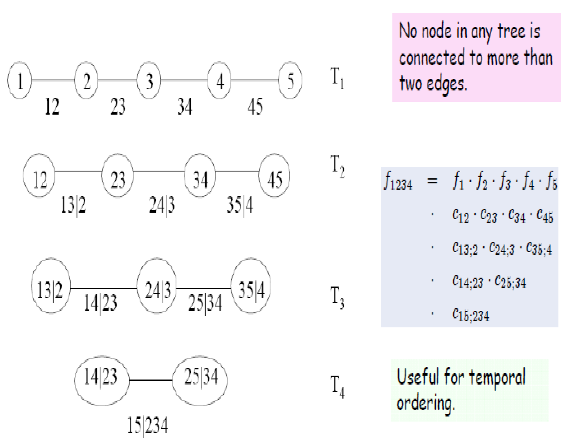
Figure 1 provides an example of two different vine structures, with a regular vine on the left and a non-regular vine on the right, both for four variables.
A vine V on n variables is a nested set of connected trees where the edges of tree j are the nodes of tree . A regular vine on n variables is a vine in which two edges in tree j are joined by an edge in tree only if these edges share a common node, . Kurowicka and Cook [26] provide the following definition of a Regular vine.
Definition 1.
(Regular vine)
V is a regular vine on n elements with denoting the set of edges of V if
- is a connected tree with nodes , plus edges ; for is a tree with nodes ,
- (proximity) for , where ∩ denotes the symmetric difference operator and # denotes the cardinality of a set.
An edge in a tree is an unordered pair of nodes of or equivalently, an unordered pair of edges of . By definition, the order of an edge in tree is . The degree of a node is determined by the number of edges attached to that node. A regular vine is called a , or C-vine, if each tree has a unique node of degree and therefore, has the maximum degree. A regular vine is termed a D-vine if all the nodes in have degrees no higher than 2.
Definition 2.
(The following definition is taken from Cook et al., (2011) [27]). For the constraint set associated with e is the complete union of of e, which is the subset of reachable from e by the membership relation.
For if , then the conditioning set associated with e is
and the conditioned set associated with e is
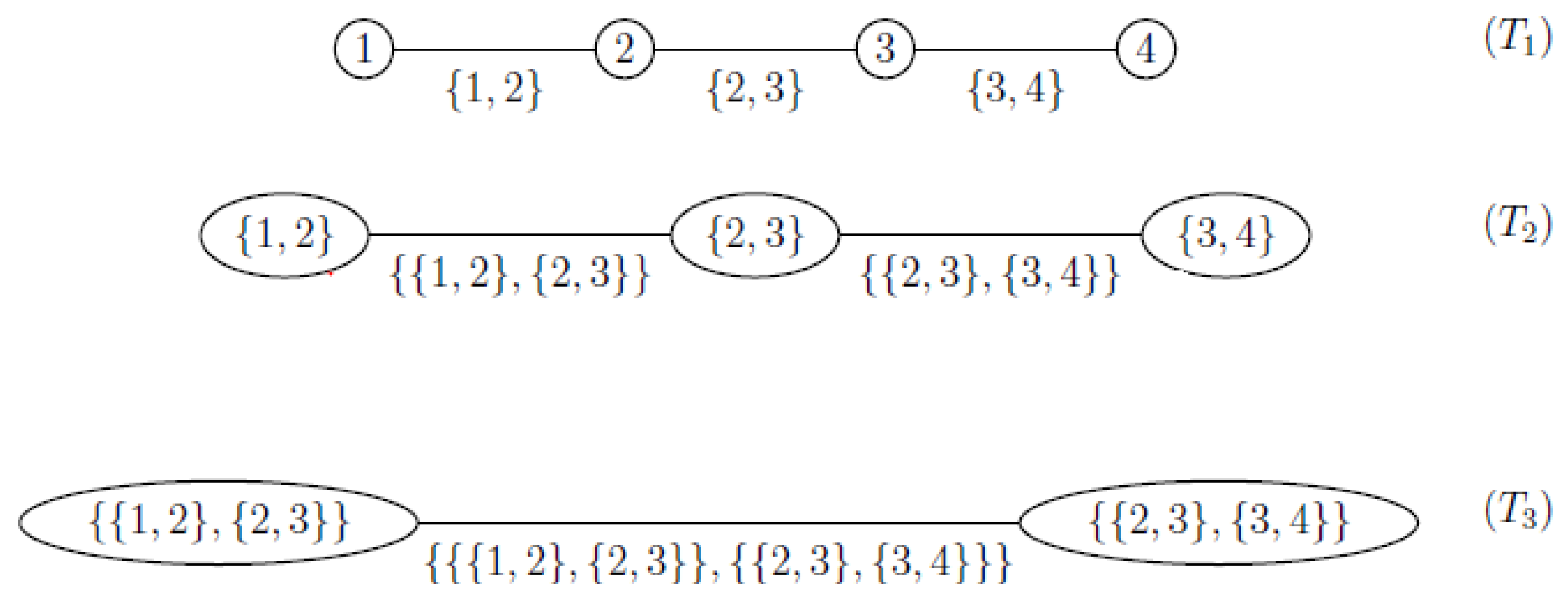
Figure 2 below shows a D-Vine with 5 dimensions.
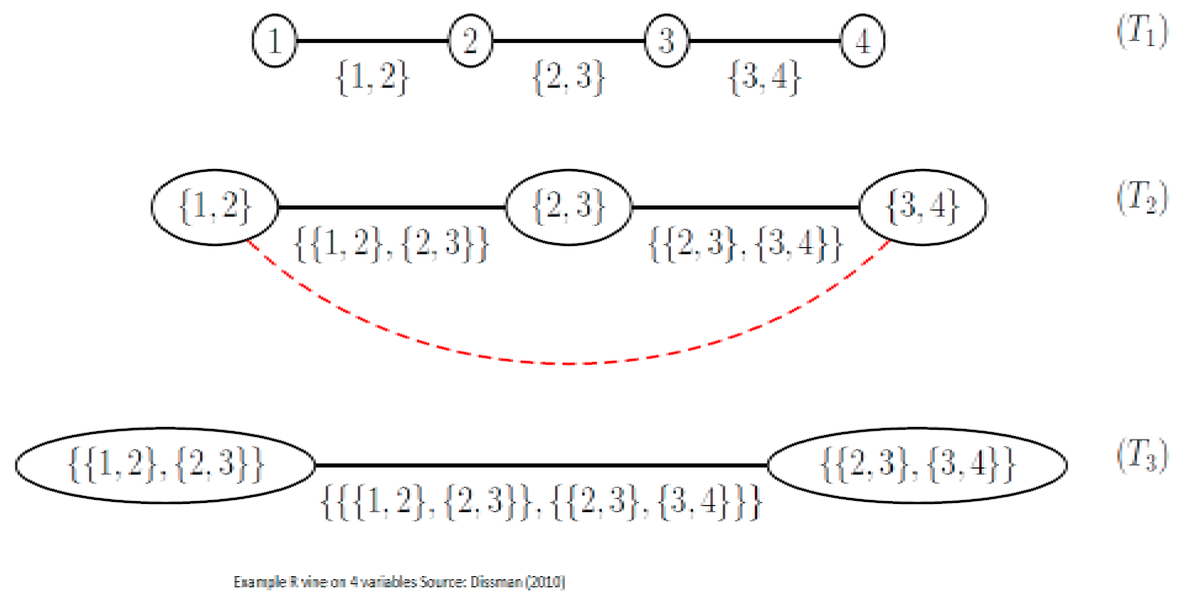
Figure 3 shows an R-Vine on 4 variables, and is sourced from Dissman (2010) [28]. The node names appear in the circles in the trees and the edge names appear below the edges in the trees. Given that an edge is a set of two nodes, an edge in the third tree is a set of a set. The proximity condition can be seen in tree , where the first edge connects the nodes and , and both share node 2 in tree .
2.1. Modelling Vines
Vine structures are developed from pair-copula constructions, in which pair-copulas are arranged in trees (in the form of connected acyclic graphs with nodes and edges). At the start of the first C-vine tree, the first root node models the dependence with respect to one particular variable, using bivariate copulas for each pair. Conditioned on this variable, pairwise dependencies with respect to a second variable are modelled, the second root node. The tree is thus expanded in this manner; a root node is chosen for each tree and all pairwise dependencies with respect to this node are modelled conditioned on all previous root nodes. It follows that C-vine trees have a star structure. Brechmann and Schepsmeier (2012) [29] use the following decomposition in their account of the routines incorporated in the R Library CDVine, which was used for the empirical work in this paper. The multivariate density, the C Vine density w.l.o.g. root nodes 1, ..., d,
where denote the marginal densities and bivariate copula densities with parameter(s) (in general, ). The outer product runs over the trees and root nodes i, while the inner product refers to the pair copulas in each tree .
D-Vines follow a similar process of construction by choosing a specific order for the variables. The first tree models the dependence of the first and second variables, of the second and third, and so on, ... using pair copulas. If we assume the order is then first the pairs (1, 2), (2, 3), (3, 4) are modelled. In the second tree, the co-dependence analysis can proceed by modelling the conditional dependence of the first and the third variables, given the second variable; the pair , and so forth. This process can then be continued in the next tree, in which variables can be conditioned on those lying between entries in the first tree, for example, the pair . The D-Vine tree has a path structure which leads to the construction of the D-vine density, which can be constructed as follows:
The outer product runs over trees, while the pairs in each tree are determined according to the inner product. The conditional distribution functions can be obtained for an vector . This can be done in a pair copula term in tree by using the pair-copulas of the previous trees and by sequentially applying the following relationship:
where is an arbitrary component of , and denotes the - dimensional vector excluding . The bivariate copula function is specified by with parameters specified in tree m.
The model of dependency can be constructed in a very flexible way because a variety of pair copula terms can be fitted between the various pairs of variables. In this manner, asymmetric dependence or strong tail behaviour can be accommodated. Figure 3 shows the various copulae available in the CDVine library in R.
2.2. Regular Vines
Until recently, the focus had been on modelling using C and D vines. However, Dissmann [28] has pointed the direction for constructing regular vines using graph theoretical algorithms. This interest in pair-copula constructions/regular vines is doubtlessly linked to their high flexibility as they can model a wide range of complex dependencies.
Figure 4 shows an R-Vine on 4 variables, and is sourced from Dissman [28]. The node names appear in the circles in the trees and the edge names appear below the edges in the trees. Given that an edge is a set of two nodes, an edge in the third tree is a set of a set. The proximity condition can be seen in tree , where the first edge connects the nodes and , plus both share the node 2 in tree .
The drawback is the curse of dimensionality: the computational effort required to estimate all parameters grows exponentially with the dimension. Morales-N poles et al. [30] demonstrate that there are possible R-Vines on n nodes. The key to the problem is whether the regular vine can be either truncated or simplified. Brechmann et al. [28] (p. 2) discuss such simplification methods. They explain that: “by a pairwisely truncated regular vine at level K, we mean a regular vine where all pair-copulas with conditioning set equal to or larger than K are replaced by independence copulas”. They pairwise simplify a regular vine at level K by replacing the same pair-copulas with Gaussian copulas. Gaussian copulas mean a simplification since they are easier to specify than other copulas, easy to interpret in terms of the correlation parameter, and quicker to estimate.
They identify the most appropriate truncation/simplification level by means of statistical model selection methods; specifically, the AIC, BIC and the likelihood-ratio based test proposed by Vuong (1989) [31]. For R-vines, in general, there are no expressions like Equations (2) and (3). This means that an efficient method for storing the indices of the pair copulas required in the joint density function, as depicted in Equation (4), is required; (4) is a more general case of (2) and (3).
Kurowicka [32] and Dissman [28] have suggested a method of proceeding which involves specifying a lower triangular matrix , with This means that the diagonal entries of M are the numbers in descending order. In this matrix, each row proceeding from the bottom represents a tree, the diagonal entry represents the conditioned set and by the corresponding column entry of the row under consideration. The conditioning set is given by the column entries below this row. The corresponding parameters and types of copula can be stored in matrices relating to M. The following example in Figure 5 is taken from Dissman [28].
The first section of Figure 5 provides a key to indicate the 5 different types of copulas used in this example, ranging from Gaussian (1) to Frank (5). The second lower triangular matrix shows the application of particular types of copulas in the trees, shows the parameters estimated, and provides the extra parameters needed when we apply the t copula.
In Figure 6 the bottom row of corresponds to , the second row to , and so on. In order to determine the edges in , we combine the numbers in the bottom row with the diagonal elements in the corresponding columns, for example the edges are (4, 3), (5, 2), (1, 2) and so on. In order to determine the edges in , we combine the numbers in the second row from the bottom with the diagonal elements in the corresponding columns and condition on the elements in the bottom row. This would give edges , and so on The final entry is given by the upper entries to the left of the matrix
2.3. Prior Work with R-Vines
The literature was initially mainly concerned with illustrative examples, (see, for example, Aas et al. [7], Berg and Aas [11], Min and Czado [12] and Czado et al. [33]). Mendes et al., (2010) [34] use a D-Vine copula model to a six-dimensional data set and consider its use for portfolio management. Dissman [28] uses R-Vines to analyse dependencies between 16 financial indices covering different European regions and different asset classes, including five equity, nine fixed income (bonds), and two commodity indices. He assesses the relative effectiveness of the use of copulas, based on mixed distributions, t distributions and Gaussian distributions, and explores the loss of information from truncating the R-Vine at earlier stages of the analysis and the substitution of independence copula. He also analyses exchange rates and windspeed data sets with fewer variables.
The research in this paper extends the work of Dissman [28] applying R-Vines to a European financial data set using a set of eleven European stock indices and features an exploration of how their dependency structures change through periods of extreme stress as represented by the GFC. The paper also features an example of how the dependencies captured by the R-Vine analysis can be used to assess portfolio Value at Risk (VaR) in a manner that closely parallels Breckmann and Czado [35] who adopted a factor model approach discussed below.
There have been other studies on European stock return series: Heinen and Valdesogo [10] constructed a CAPM extension using their Canonical Vine Autoregressive (CAVA) model using marginal GARCH models and a canonical vine copula structure. Breckmann and Czado [35] develop a regular vine market sector factor model for asset returns that uses GARCH models for margins, and which is similarly developed in a CAPM framework. They explore systematic and unsystematic risk for individual stocks, and consider how vine copula models can be used for active and passive portfolio management and VaR forecasting.
3. Sample
We use a data set of daily returns, which runs from 1 January 2005 to 31 January 2013 for ten European indices and the composite blue chip STOXX50 European index. We use the British FTSE 100 Index, the German DAX Index, the French CAC 40 Index, the Netherlands AEX Amsterdam Index, the Spanish Ibex 35 Index, the Danish OMX Copenhagen 20 Index, the Swedish OMX Stockholm All Share Index, the Finnish OMX Helsinki All Share Index, the Portuguese PSI General Index, and the Belgian Bell 20 Index. As a composite European market index we use the STOXX 50. This index covers 50 stocks from 12 Eurozone countries: Austria, Belgium, Finland, France, Germany, Greece, Ireland, Italy, Luxembourg, the Netherlands, Portugal and Spain. We divide our sample into returns for the pre-GFC (January 2005–July 2007), GFC (July 2007–September 2009) and post-GFC (September 2009–December 2013) periods. The sample is shown in Table 1.
Table 2 and Table 3 provide descriptive statistics for the ten European market indices and the composite European STOXX50 index broken down into our three periods; pre-GFC (January 2005–July 2007), GFC (July 2007–September 2009) and post-GFC (September 2009–December 2013). It is apparent that the mean and median returns are uniformly positive in the pre-GFC period, and uniformly negative in the GFC period, whilst the median return is either zero or positive for all but two of the indices during this period. In the post-GFC the mean and median returns for most markets are positive or zero except in the cases of the Spanish and Portuguese markets where there are negative mean returns. The standard deviation is higher in all markets in the GFC period. The Bera-Jarque test significantly rejects normality of the daily return distributions for all indices in all periods. The returns are skewed but in many cases change the direction of the skew from positive to negative in different periods. Only three markets display negative skewness in the GFC period; the Danish, the Portuguese and the Belgian markets. All markets except the Swedish one show greater excess-kurtosis during the GFC period. The GFC period is also characterised by a higher value of the Hurst exponent in all markets, with a value greater than 0.57 in all markets, suggesting the markets display long memory in times of crisis.
The descriptive statistics provided in Table 2 and Table 3 suggest that the European index return series in our sample are non-Gaussian and are subject to changes in skewness and kurtosis in the different sample sub-periods. This suggests they should be amenable to analysis by copulas which may capture the effects of fat tails and changes in distributional characteristics.
4. Results
The results are presented here in two parts. In the first subsection below we model the dependence structure of the European set of indices, in three subperiods covering GFC. The second subsection gives results from an empirical exercise modelling VaR using R-Vine Copulas for a 10 asset portfolio and contrasts it with the results of a more traditional Gaussian approach undertaken in a GARCH framework.
4.1. Dependence Modelling Using Vine Copula
We divide the data into three time periods covering the pre-GFC (January 2005–July 2007), GFC (July 2007–September 2009), and post-GFC periods (September 2009–December 2011) to run the C-Vine and R-Vine dependence analysis for the stocks comprising Dow Jones Index. Before we can do this we require appropriately standardised marginal distributions for the basic company return series. These appropriate marginal time series models for the Dow Jones data have to be found in the first step of our two step estimation approach. The following time series models are selected in a stepwise procedure: GARCH (1, 1), ARMA (1, 1), AR(1), GARCH(1, 1), MA(1)-GARCH(1, 1). These are applied to the return data series and we select the model with the highest p-value, so that the residuals can be taken to be i.i.d. The residuals are standardized and the marginals are obtained from the standardized residuals using the Ranks method. These marginals are then used as inputs to the Copula selection routine. The copula are selected using the AIC criterion. We first discuss the results obtained from the pre-GFC period data followed by the GFC and post-GFC periods.
4.2. Pre-GFC
The following Figure 7 presents the structure of the C-Vines.
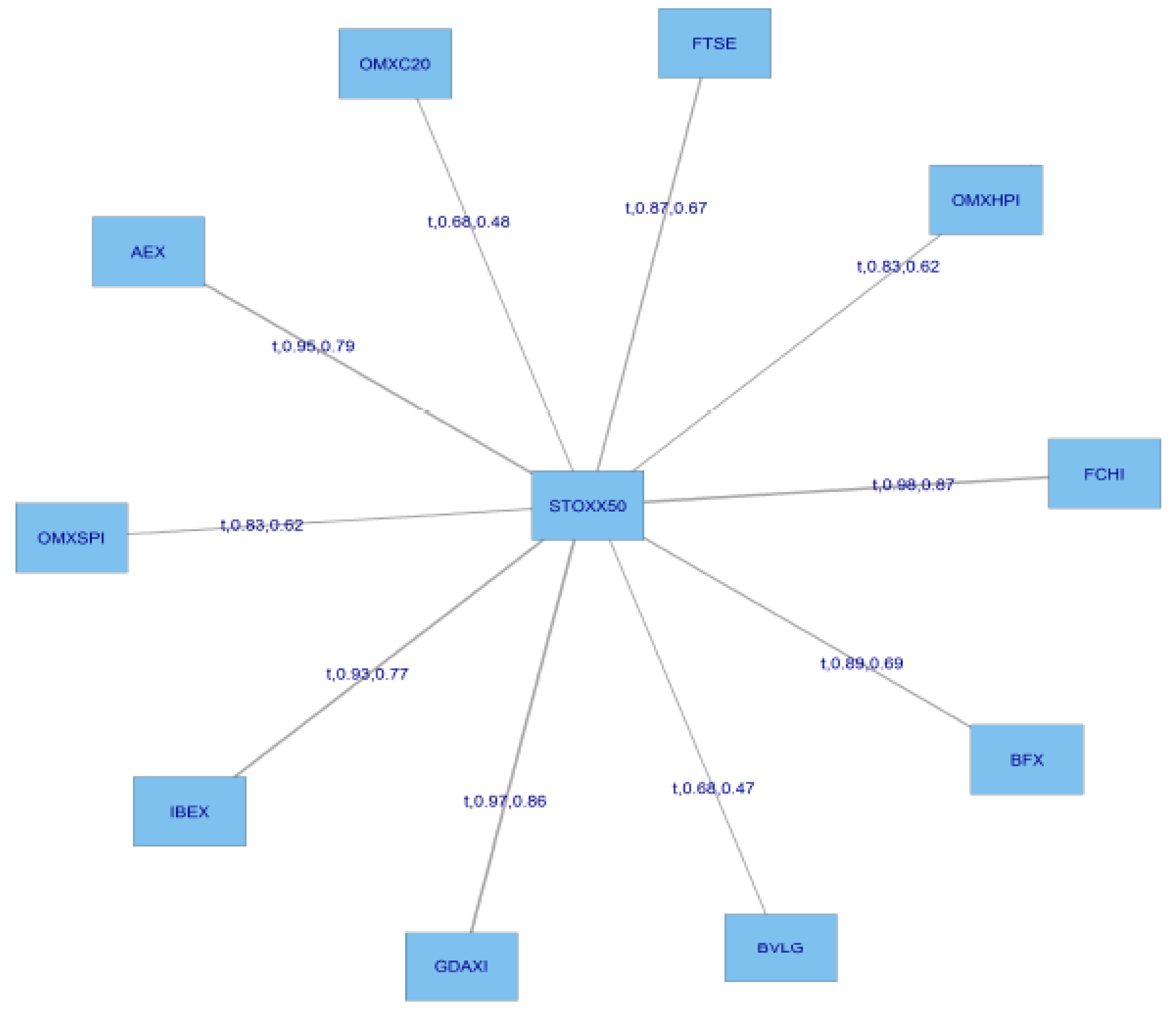
For this C Vine selection, we choose as root node the node that maximizes the sum of pairwise dependencies to this node.We commence by linking all the stocks to the STOXX50 index which is at the centre of this diagram. We use a range of Copulas from for selection purposes; the range being (1:6). We apply AIC as the selection criterion to select from the following menu of copulae: 1 = Gaussian copula, 2 = Student t copula (t-copula), 3 = Clayton copula, 4 = Gumbel copula, 5 = Frank copula, 6 = Joe copula.
We then compute transformed observations from the estimated pair copulas and these are used as input parameters for the next trees, which are obtained similarly by constructing a graph according to the above C-Vine construction principles (proximity conditions), and finding a maximum dependence tree. The C-Vine tree for period 2 is shown Figure 8.
The pre-GFC C-Vine copula specification matrix is displayed in Table 4 below. It can be seen from the top and bottom of the first column in Table 4 that in the pre-GFC period the strongest correlations are between the FTSE and Belgian Index BFX. The BFX remains at the bottom across all columns in the last row of Table 4.
From Table 4, it can be seen that the strongest individual correlations in the pre-GFC period, are between the FTSE at the top of the first column, BFX in the final row, and the individual diagonal entries starting with the FTSE at the top of the first column, which define the edges. The FTSE is correlated with BVLG (security 11), then conditioned by its relationship with OMXHPI (security 8), the Helsinki exchange index, then OMXSPI (security 5), the Stockholm index, then OMXC20 (security 3), the Copenhagen index, and so on. It can also be seen in Table 2 that C Vines are less flexible in that the same security number can usually be seen to appear across the rows. This means that it is always appearing in the nodes at that level in the tree. R Vines are more flexible and do not have this requirement. Later in the paper, we will concentrate on the results of the R Vine analysis.
Table 5 shows which copula are fitted to capture dependencies between the various pairs of indices. At the bottom of column 1 in Table 5 we can see that number 2 copula, the Student t copula is applied, to capture the dependency between FTSE and BFX, and then it is conditioned by the relationship with BVLG but this relationship uses a Frank copula (5), and so forth. All 6 categories of copula are used in Table 5 but the Student t copula appears most frequently in the table, followed by the Frank copula, the Gaussian copula, the Clayton copula and finally the Joe copula and the Gumbel copula appear once each.
It can be seen in Table 6 in the entries in the bottom row that there are strong positive dependencies between subsets of the markets concerned. The entry in the bottom of the first column shows the strong positive dependency between the FTSE and BFX. All the entries in the bottom row of Table 6 are strongly positive. We can see in the first column, that once we have conditioned the FTSE on its relationships with the markets in the bottom half of the column it is strongly positively related to the STOXX50. Not all the dependencies indicated in Table 6 are positive though, and there are 11 cases of negative co-dependency, once the relationship across other nodes has been taken into account.
Table 7 shows the second set of parameters, in cases where one is needed, for example the Student t copula.
Table 8 shows the tau matrix for the C Vine copulas in the pre-GFC period.
The bottom row of Table 8 captures the strongest dependencies between the pairs of markets, as represented by their respective indices.
A key concern in this paper is the issue of how dependencies have changed as a result of the GFC?
4.3. GFC Period
Figure 9 shows tree 1 for C-Vine copula estimates in the GFC period, and Figure 10 shows tree 2 for the same period.
We are interesting in examing whether the major financial shock which constituted the GFC caused a noticeable change in dependencies?
Table 9 and Table 10 depicts the copulas chosen to capture dependency relationships during the GFC period.
A comparison of the entries in Table 10, the copula specification matrix for the GFC, with those in Table 5, the pre-GFC copula specification matrix, reveals that there is much less us of Gaussian copulas, 3 in Table 10, compared with 11 in Table 5. There is now a much greater use made of the Student T copula, on 36 occasions in Table 10, compared with 18 in Table 5. The use of the Gumbel copulas has increased from 1 to 4 occasions and the Clayton copula is only used on 2 occasions compared with 5 pre-GFC. The use of the Frank copula has declined from 15 to 6, whilst the Joe copula, now makes 2 appearances compared to 1 pre-GFC. The massive expansion of the use of the Student t copula, together with the other changes mentioned, is consistent with greater weight being placed on the tails of the distribution durng the GFC period.
The dependencies are captured in the Tau matrix shown in Table 11. A comparison of the values in Table 11, the tau matrix for the GFC, with those in Table 8, the tau matrix for the GFC period, reveals that the relationships have become more pronounced. If we look at the dependencies in the bottom row of Table 11, in 7 from the total of 10 cases the dependencies have increased. It is also true that there has also been a marginal increase in negative dependencies, from 10 pre-GFC to 12 during the GFC, but the values of these are of a low order. The picture that emerges from Table 11 is one of an increase in dependencies between these major European stock markets during an economic down-turn.
4.4. Post-GFC Period
We will now turn our attention to the post-GFC period. In the case of the European markets, this is likely to be less-clear cut, given that it was characterised by economic turmoil related to the subsequent post-GFC European Sovereign debt crisis. Figure 11 displays the first tree post-GFC, and Figure 12 the second tree.
Table 12 shows the post-GFC C-Vine copula structure, and Table 13 the post-GFC C-Vine Copula Specification Matrix.
It can be seen in Table 13 that there is a marked change in the type of copula used to capture dependencies in the post-GFC period. The use of the Gaussian copula has risen from 3 during the GFC period to 10 in the post-GFC period, and the application of the Student t copula has dropped from 36 during the GFC to 24 in the post GFC period, whilst the use of the Clayton copula in the post-GFC period rises to 8 from 2 in the GFC period. The Gumbel copula is used on 6 occasions, whilst the Frank copula appears only 5 times, compared with 15 in the pre-GFC period. Finally, the Joe copula, is made use of on 1 occasion. The increase in the use of the Gaussian copula and the reduction in the use of the Student t copula suggests there is much less emphasis on the tails of the distributions in the post-GFC period.
The post-GFC tau matrix is shown in Table 14. The structure of dependencies that emerges in Table 14 is quite complex when compared to those of the GFC period. In the bottom row the positive dependencies captured in the tau statistics have increased in 7 of the total of 10 cases. In the GFC period there were 12 negative tau coefficients in the matrix, where as in the post-GFC period this number has reduced to 10. Thus, the broad picture that emerges in the post-GFC period, based on the use of C-Vine copulas, is that overall dependencies increased in the post-GFC period across the major European markets, in association with their experience of the European Sovereign debt crisis. The greater use of Gaussian copulas and the reduction in the use of Student t copulas in this period, suggests that tail behaviour was less important.
We now switch to the more flexible R-Vine framework to compare the two approaches.
5. R Vine Copulas
5.1. The Pre-GFC Period
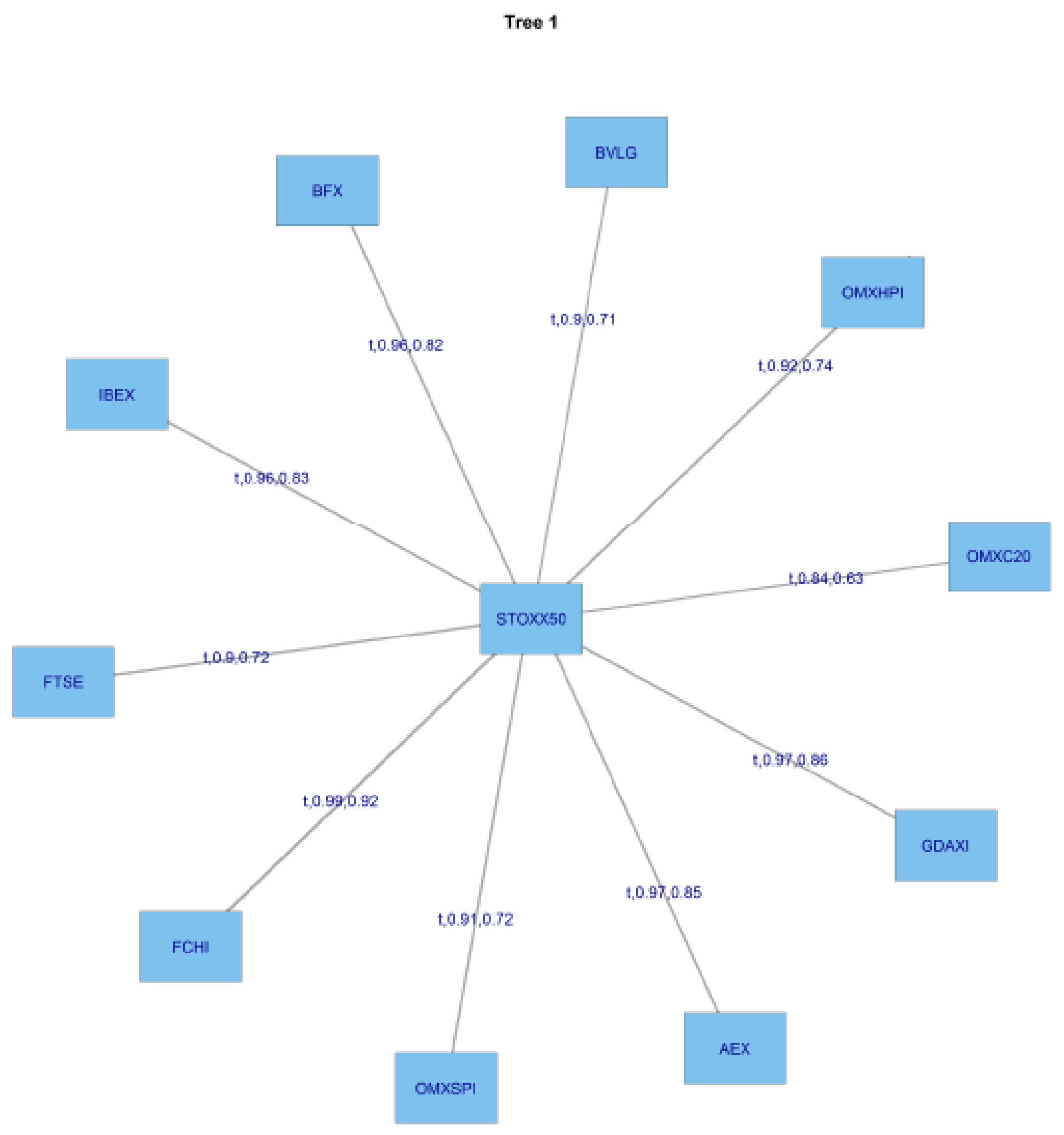
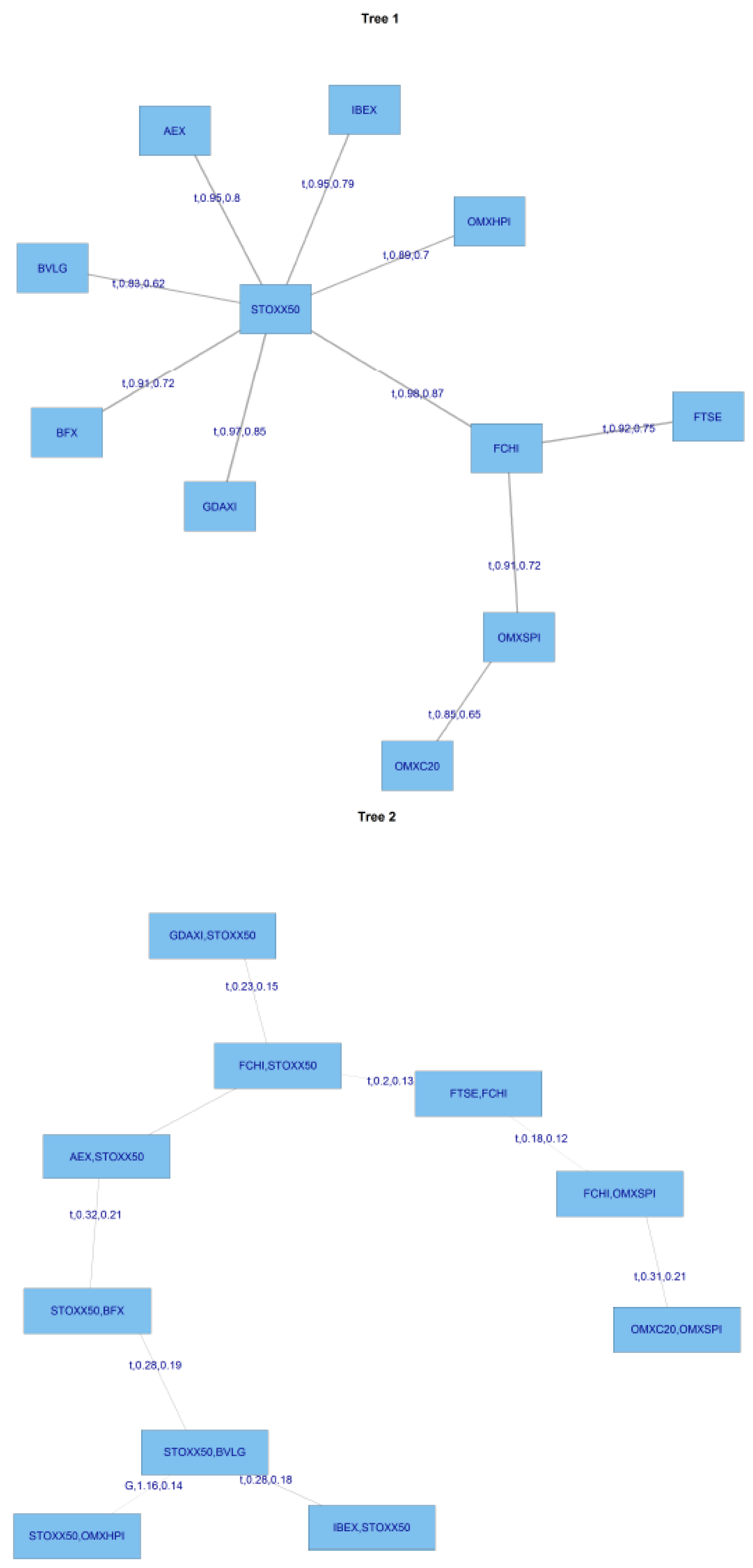
It can be seen in Figure 13 and Figure 14 above that the R Vine structure is more flexible. Tree 1 shows that a sub-group of the European markets are linked together; namely the Portuguese (BVLG), Brussels (BFY), the French (FCHI) and the Danish (OMXC20), they are then linked to the European Index (STOXX50). The other markets; Amsterdam (AEX), Germany (GDAXI), Stockholm (OMXSPI), Spain (IBEX), the UK (FTSE), and Helsinki (OMXHPI), have the strongest co-dependency with the European Index (STOXX50). This is also apparent in Table 15 and Table 16 which show.
Table 15 shows the types of copulas fitted in the empirical analysis.
The advantage of the use of R Vines is apparent in Table 15. Complex patterns of dependency can be readily captured. It can be seen that at different dependencies conditioned across the same node six different copulas are used. For example, in column 1 the first copula used is the Clayton copula (no 3), followed by the Frank copula (no 5) for a couple of levels, then the Joe Copula (no 6), the Frank copula (no 5), two cases of the Gaussian (no 1), then the Gumbel (no 4), then the Frank copula again, and finally, the Student t (no 2). This variety of usage is apparent across Table 15 at various levels in the tree structures used to capture dependencies. The bottom row consists entirely of Student t copulas.
The copulas used to capture co-dependencies are different from the pre-GFC period C-Vine analysis. In that case, illustrated in Table 4; 11 Gaussian, 18 Student t copulas, 5 Clayton copulas, I Gumbel, 15 Frank copulas, and 1 Joe Copula were used. By contrast, in Table 15, 11 Gaussian, 18 Student t, 9 Clayton, 3 Gumbel, 12 Frank and 1 Joe copula are used. This follows, given that different co-dependencies are captured in the tree because there are not constraints on the pairings in R Vine copulas.
In the interests of brevity the details of the parameters estimated are not tabulated but the tau matrix, is shown in Table 16. The entries in Table 16 for R-Vines can be contrasted with those in Table 8 for C-Vines. Once again, given the nature of the analysis, the strongest dependencies between the various indices are captured by the entries in the bottom row of the table. Overall, the picture of dependencies is similar to those captured by the C-Vine analysis. The biggest change is in the first column of Table 16 in that the relationships between the FTSE and STOXX50, OMXC20 and OMXSPI have now become negative, but it has to be born in mind that the relationship is now conditioned on the much stronger relationship between the FTSE and BFX.
5.2. R-Vines GFC
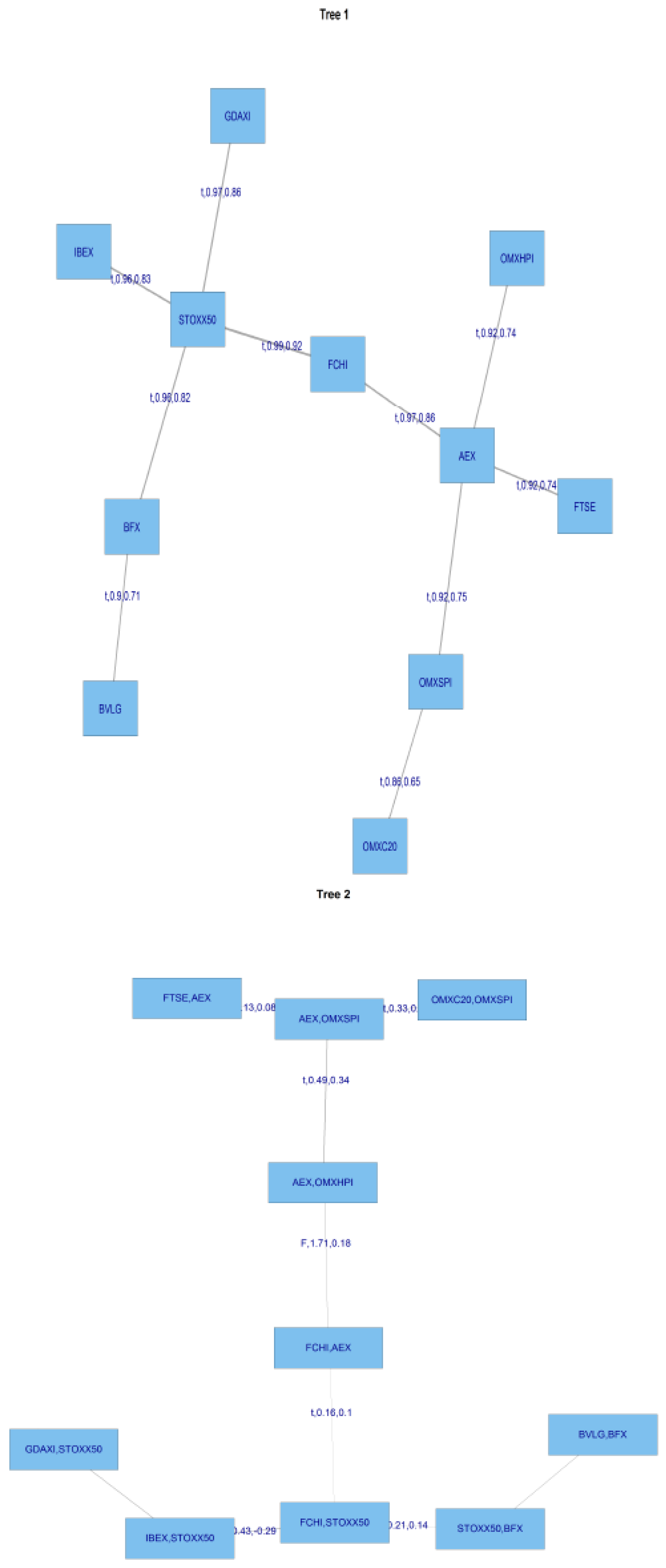
Figure 15 provides the trees for the R-Vine analysis in the GFC period.
The trees shown in Figure 16 indicate that dependencies have changed because of the influence of the GFC and the FTSE is now linked via the French FCHI to the STOXX50, whilst the OMXC20 and OMXSPI are now linked via the FCHI to the STOXX50. Previously, in the pre-GFC period the BVLG and the BFX were linked by the FCHI, but this is no longer the case.
Table 17 once again suggests the importance of capturing tail risk in financial and economic downturns plus the importance of fat-tailed distributions. Only 4 Gaussian copulas are applied in Table 17, where as the Student t copula dominates, being used on 38 occasions. There are 2 applications of the Clayton copula, 5 of the Gumbel and 4 of the Frank, whilst the Joe copula is used on 1 occasion.
Table 18 provides details of the tau matrix for the GFC period. The change in dependencies in the R-Vine analysis following the GFC is complex and difficult to interpret in a clear-cut fashion. In terms of the dependencies captured in the bottom row of Table 18, 5 show and increase in their values, compared with the pre-GFC entries in Table 1, 6 but 5 also show a decrease. In terms of the whole matrix, the number of negative entries in Table 18 is 10, the same as the number in Table 16, but because of complex changes in patterns of dependencies, they now occur at predominantly different positions in the matrix.
We will therefore move on to the post-GFC R-Vine analysis.
5.3. Post-GFC R-Vines
Figure 17 shows the R-Vine trees in the post-GFC period. Figure 17 reveals that the relationships between the markets have changed in a complex manner in the post GFC period. It can be seen in tree 1 that the FTSE is now linked to the STOXX50 via the Dutch and French Indices. The Finnish, Danish and Swedish markets are also linked via the Durch and French markets to the STOXX50. The German and Spanish markets have individual links to the STOXX50, whilst the Portuguese market is linked via the Belgian index to the STOXX50. Table 19 shows the types of copulas used to map dependencies in the post-GFC period.
The Gaussian copula is used on 9 occasions whilst the Student t copula again dominates with 25 entries in Table 19, a considerable reduction on the 38 times it was applied during the GFC period. The Clayton copula appears 4 times, the Gumbel on 2 occasions. Greater use is made of the Frank copula, which appears 8 times and finally the Joe copula is used on 4 occasions.
The tau dependency matrix is shown in Table 20.
The tau matrix in Table 20 shows that dependencies have again changed in a complex manner in the post-GFC period which coincides with the European Sovereign debt crisis. The large dependencies in the bottom row have increased in 6 of the 10 cases in the post-GFC period. However, there are 12 cases of negative relationships in Table 20 as opposed to 8 in Table 18 representing the GFC period. These changes are interesting but do not give a direct indication of the usefulness of R-Vine modelling. We undertake an empirical application in the next section, which features a Value at Risk, (VaR) analysis, and this provides an illustration of its use in risk-assessment.
Fink et al., (2017) [36] use a Markov-switching R-vine model to explore the existence of different global dependence regimes. They explore the relationships between stock and volatility indices in Asia, Europe and the USA. They confirm the presence of normal and abnormal regimes. Our analysis is different in that we choose a particular time period to represent the GFC, whereas they use smoothed rolling windows, in an attempt to tease out changes in parameters in a Markov-switching analysis. They mention greater reliance on the Gumbel copula in the GFC period which we similarly note becomes more prominent in this period.
There are some further limited parallels between our work and that of Beil (2013) [37], who applies vine copula analysis to global indices and includes the DAX and STOXX in a broader global analysis which includes a separate period for 2007–2008, which is designated as the GFC period. However, Beil [37] makes relatively less use of the Gumbel copula in the truncated crisis period of this analysis. Furthermore, the overall sample of indices used is very different, and includes both US and Asian stock indices, and their corresponding volatility indices.
6. An Empirical Application
Empirical Example
We have used C-Vine and R-Vine Copulas to map dependence structures between some of the major European markets. These, in turn, can be used for portfolio evaluation and risk modelling. The R-Vine approach potentially gives better results than usual bivariate copula approach given that the copulas selected via Vine copulas are more sensitive to the asset’s return distributions.
The co-dependencies calculated by R-Vine copulas can be used for portfolio Value at Risk quantification. We construct an equally weighted portfolio of the eleven market indices to explore the use of Vine copulas in modelling VaR using a portfolio example. The data used for this part of the analysis is from 3 January 2010 to 31 December 2011 with total 504 returns per asset, the eleven selected assets in the portfolio are our eleven European market indices. We use a 250 days moving window dynamic approach to forecast the VaR for this equally weighted portfolio which results in 254 forecasts. The main steps of the approach are as outlined below:
- Convert the data sample to log returns.
- Select a moving window of 250 returns.
- Fit GARCH(1,1) with Student-t innovations to convert the log returns into an i.i.d. series. We fit the same GARCH(1,1) with student-t in all the iterations to maintain uniformity in the method, and this approach also makes the method a little less computationally intensive.
- Extract the residuals from Step-3 and standardize them with the Standard deviations obtained from Step-3.
- Convert the standardized residuals to student-t marginals for Copula estimation. The steps above are repeated for all the 10 stocks to obtain a multivariate matrix of uniform marginals.
- Fit an R-Vine to the multivariate data with the same copulas as used in Section 1.
- Generate simulations using the fitted R-Vine model. We generate 1000 simulations per stock for forecasting a day ahead VaR.
- Convert the simulated uniform marginals to standardized residuals.
- Simulate returns from the simulated standardized residuals using GARCH simulations.
- Generate a series of simulated daily portfolio returns to forecast 1% and 5% VaR.
- Repeat step 1 to 10 for a moving window.
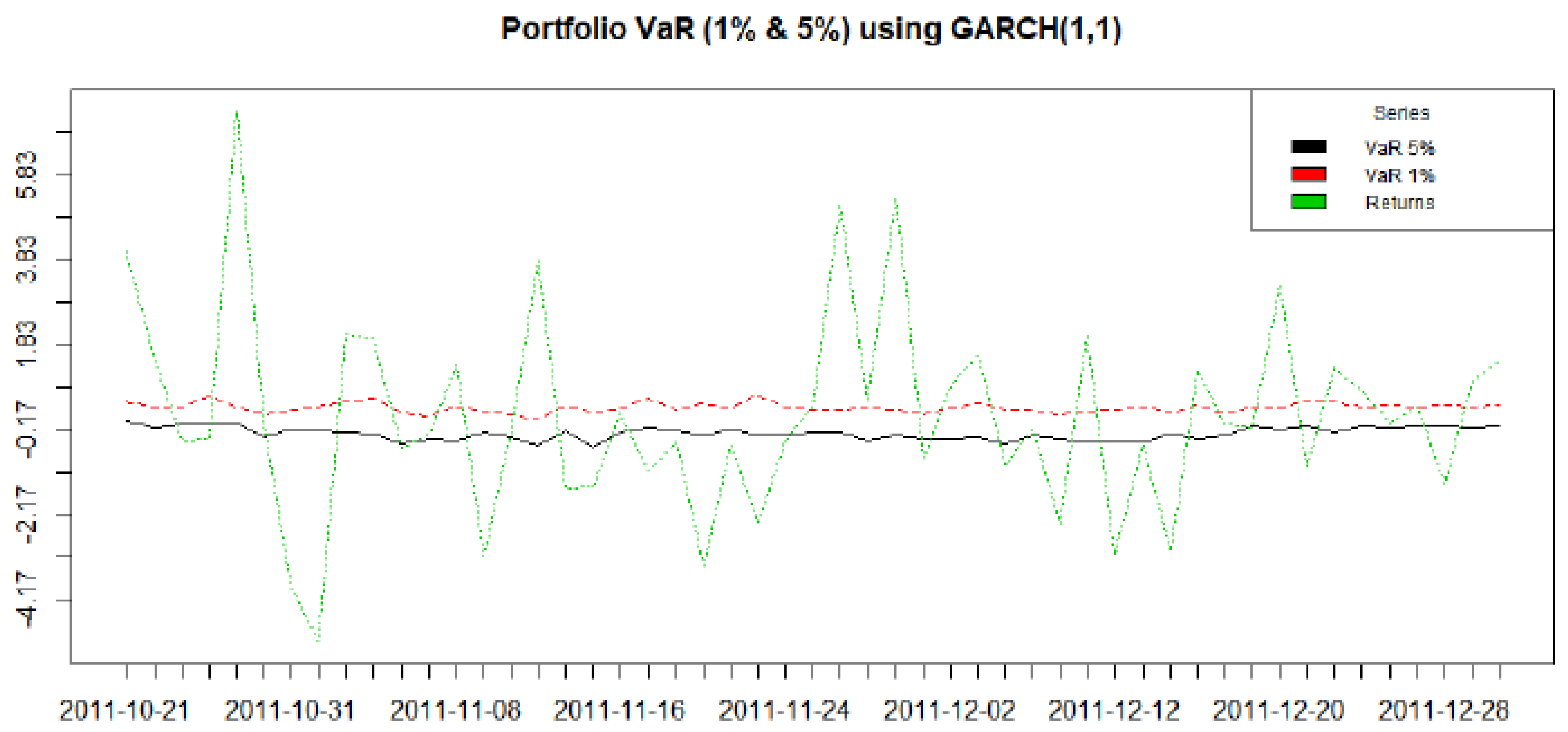
The approach above results in VaR forecasts which whilst not dependent in time have the advantage of being co-dependent on the stocks in the portfolio. We use this approach as a demonstration of a practical application of the information about co-dependencies captured by the flexible Vine Copula approach applied to construct VaR forecasts. Figure 18 and Table 21 plots the 1% and 5% VaR forecasts along with original portfolio return series obtained from the method. The plot shows that the VaR forecasts closely follow the daily returns with few violations.
Table 13 below gives the results from Unconditional Coverage (Kupiec) and Conditional Coverage (Christoffersen) (Christoffersen [38] and Christoffersen, Hahn & Inoue, 2001 [39]) which are based on the number of VaR violations compared to the actual portfolio returns. According to the results in the table both the tests accept both 1% and 5% VaR models for the forecasting period.
As a direct contrast we also use our series of index returns combined into an equally weighted portfolio to construct a simulation of a VaR analysis based on the use of a GARCH(1, 1) model. The relative number of violations of the VaR set at 1% and 5% should indicate whether our vine copula approach better captures the complex structure of dependencies and is better suited to VaR analysis.
We proceed as follows:
- Convert the data sample to log returns.
- Select a moving window of 250 returns.
- Fit GARCH(1,1) with Normal innovations to convert the log returns into an i.i.d. series.
- Extract the fit from step-3 and simulate 1000 returns per asset.
- Repeat step-3 and 4 for all the stocks and then calculate the portfolio return from the simulated series.
- Generate a series of simulated daily portfolio returns to forecast 1% and 5% VaR.
- Repeat step 1 to 10 for a moving window.
A plot of the results of this exercise is shown in Figure 19 and Table 22. A brief glance at this shows that the application of a GARCH(1,1) model and the Gaussian distribution leads to multiple violations of the VaR 5 per cent (black line) and the VaR 1 percent (red line), whereas the VaR calculated on the basis of vine copulas, as shown in Figure 18, lead at most, to two breaches of the VaR.
7. Conclusions
In this paper we used the recently developed R Vine copula methods (see Aas et al. [7], Berg and Aas [11], Min and Czado [12] and Czado et al. [33]) to analyse the changes in the co-dependencies of ten European stock market indices and the composite STOXX50 index for three periods spanning the GFC: pre-GFC (January 2005–July 2007), GFC (July 2007–September 2009) and post-GFC periods (September 2009–December 2013). The results suggest that the dependencies change in a complex manner and there is evidence of greater reliance on the Student t copula in the copula choice within the tree structures for the GFC period which is consistent with the existence of larger tails to the distributions of returns. One of the attractions of this approach to risk-modelling is the flexibility available in the choice of distributions used to model co-dependencies. We demonstrated the calculation of portfolio VaR on the basis of these dependency measures and the method appears to work well on the basis of coverage ratio tests, which do not reject the null hypthesis in back-tests. This contrasts with the results on simulations to the same data set based on a GARCH(1, 1) model and the Gaussian distribution.
The main limitation is the static nature of the approach and dynamic applications are in the process of development. Breckmann and Czado [16] have proposed a COPAR model which provides a vector autoregressive VAR model for analysing the non-linear and asymmetric co-dependencies between two series. A more dynamic approach will be the subject of future work.
Acknowledgments
For financial support, the authors wish to thank the Australian Research Council. The third author would also like to acknowledge the National Science Council, Ministry of Science and Technology, Taiwan, and the Japan Society for the Promotion of Science. The authors appreciate the very helpful comments and suggestions of the two reviewers.
Author Contributions
Allen, McAleer and Singh, conceived the paper, Singh under took the analysis. Allen, McAleer and Singh wrote up the paper.
Conflicts of Interest
The authors declare no conflicts of interest.
References
- Joe, H. Multivariate Models and Dependence Concepts; Chapman & Hall: London, UK, 1997. [Google Scholar]
- Nelsen, R. An Introduction to Copulas, 2nd ed.; Springer: New York, NY, USA, 2006. [Google Scholar]
- Joe, H. Families of m-variate distributions with given margins and m(m-1)/2 bivariate dependence parameters. Lect. Notes-Monogr. Ser. 1996, 28, 120–141. [Google Scholar]
- Bedford, T.; Cooke, R.M. Probability density decomposition for conditionally dependent random variables modeled by vines. Ann. Math. Artic. Intell. 2001, 32, 245–268. [Google Scholar]
- Bedford, T.; Cooke, R.M. Vines—A new graphical model for dependent random variables. Ann. Stat. 2002, 30, 1031–1068. [Google Scholar]
- Kurowicka, D.; Cooke, R.M. Uncertainty Analysis with High Dimensional Dependence Modelling; John Wiley: Chichester, UK, 2006. [Google Scholar]
- Aas, K.; Czado, C.; Frigessi, A.; Bakken, H. Pair-copula constructions of multiple dependence. Insurance Math. Econ. 2009, 44, 182–198. [Google Scholar] [Green Version]
- Schirmacher, D.; Schirmacher, E. Multivariate dependence modeling using pair-copulas. In Proceedings of the Society of Actuaries: 2008 Enterprise Risk Management Symposium, Chicago, IL, USA, 14–16 April 2008; Available online: http://www.soa.org/library/monographs/other-monographs/2008/april/2008-erm-toc.aspx (accessed on 1 September 2017).
- Chollete, L.; Heinen, A.; Valdesogo, A. Modeling international financial returns with a multivariate regime switching copula. J. Financ. Econ. 2009, 7, 437–480. [Google Scholar]
- Heinen, A.; Valdesogo, A. Asymmetric CAPM dependence for large dimensions: The canonical vine autoregressive model. In CORE Discussion Papers 2009069; Universite catholique de Louvain: Louvain-la-Neuve, Belgium, 2009. [Google Scholar]
- Berg, D. Copula goodness-of-fit testing: An overview and power comparison. Eur. J. Financ. 2009, 15, 675–701. [Google Scholar]
- Min, A.; Czado, C. Bayesian inference for multivariate copulas using pair-copula constructions. Accept. Publ. J. Financ. Econom. 2010, 8, 511. [Google Scholar]
- Smith, M.; Min, A.; Czado, C.; Almeida, C. Modeling longitudinal data using a pair-copula decomposition of serial dependence. J. Am. Stat. Assoc. 2010, 492, 1467–1479. [Google Scholar] [CrossRef]
- Allen, D.E.; Ashraf, A.; McAleer, M.; Powell, R.J.; Singh, A.K. Financial dependence analysis: Applications of vine copulas. Stat. Neerlandica 2013, 67, 403–435. [Google Scholar]
- Patton, A.J. Copula based models for financial time series. In Handbook of Financial Time Series; Springer: Berlin/Heidelberg, Germany, 2009; pp. 767–785. [Google Scholar]
- Brechmann, E.C.; Czado, C. COPAR—Multivariate time-series model. In Working Paper; Technical University of München: München, Germany, 2012. [Google Scholar]
- Sklar, A. Fonctions de Repartition a n Dimensions et Leurs Marges; Publications de l’Institut de Statistique de L’Universite de Paris: Paris, France, 1959; Volume 8, pp. 229–231. [Google Scholar]
- Joe, H.; Li, H.; Nikoloulopoulos, A. Tail dependence functions and vine copulas. J. Multivar. Anal. 2010, 101, 252–270. [Google Scholar] [CrossRef]
- Geidosch, M.; Fischer, M. Application of vine copulas to credit portfolio risk modeling. J. Risk Financ. Manag. 2016, 9, 4. [Google Scholar] [CrossRef]
- Fischer, M.; Kraus, D.; Pfeuffer, M.; Czado, C. Stress testing German industry sectors: Results from a vine copula based quantile regression. Risks 2017, 5, 38. [Google Scholar] [CrossRef]
- Panagiotelis, A.; Czado, C.; Joe, H.; Stöber, J. Model selection for discrete regular vine copulas. Comput. Stat. Data Anal. 2017, 106, 138–152. [Google Scholar] [CrossRef]
- Bedford, T.; Daneshkhah, A.; Wilson, K.J. Approximate uncertainty modeling in risk analysis with vine copulas. Risk Anal. 2016, 36, 792–815. [Google Scholar] [CrossRef] [PubMed] [Green Version]
- Scheffer, M.; Weiss, G.N.F. Smooth nonparametric Bernstein vine copulas. Quant. Financ. 2017, 17, 139–156. [Google Scholar] [CrossRef]
- Aas, K. Pair-copula constructions for financial applications: A review. Econometrics 2016, 4, 43. [Google Scholar] [CrossRef]
- Fermanian, J.D. Recent developments in copula models. Econometrics 2017, 5, 34. [Google Scholar] [CrossRef]
- Kurowicka, D.; Cooke, R.M. A parametrization of positive definite matrices in terms of partial correlation vines. Linear Algebra Its Appl. 2003, 372, 225–251. [Google Scholar] [CrossRef]
- Cooke, R.M.; Joe, H.; Aas, K. Vines Arise Chapter 3. In DEPENDENCE MODELING Vine Copula Handbook; Kurowicka, D., Joe, H., Eds.; World Scientific Publishing Co.: Singapore, 2011. [Google Scholar]
- Dissman, J.F. Statistical Inference for Regular Vines and Application. Master’s Thesis, Technische Universitat München, München, Germany, 2010. [Google Scholar]
- Brechmann, E.C.; Schepsmeier, U. Modeling Dependence with C- and D-vine Copulas: The R-package CDVine. Available online: http://cran.r-project.org/web/packages/CDVine/vignettes/CDVine-package.pdf (accessed on 1 September 2012).
- Morales-N’apoles, O.; Cooke, R.; Kurowicka, D. About the Number of Vines and Regular Vines on n Nodes. Available online: https://repository.tudelft.nl/islandora/object/uuid:912abf55-8112-48d2-9cca-323f7f6aecc7?collection=research (accessed on 10 September 2017).
- Vuong, Q.H. Likelihood ratio tests for model selection and non-nested hypotheses. Econometrica 1989, 57, 307–333. [Google Scholar] [CrossRef]
- Kurowicka, D. Optimal truncation of vines. In Dependence Modeling: Handbook on Vine Copulae; Kurowicka, D., Joe, H., Eds.; World Scientific Publishing Co.: Singapore, 2011. [Google Scholar]
- Czado, C.; Schepsmeier, U.; Min, A. Maximum likelihood estimation of mixed C-vines with application to exchange rates. Stat. Model. 2011, 12, 229–255. [Google Scholar] [CrossRef]
- Mendes, B.V.D.M.; Semeraro, M.M.; Leal, R.P.C. Pair-copulas modeling in finance. Financ. Mark. Portf. Manag. 2010, 24, 193–213. [Google Scholar] [CrossRef]
- Brechmann, E.C.; Czado, C. Risk Management with High-Dimensional Vine Copulas: An Analysis of the Euro Stoxx 50. Stat. Risk Model. 2013, 30, 307–342. [Google Scholar] [CrossRef]
- Fink, H.; Klimova, Y.; Czado, C.; Stober, J. Regime switching vine copula models for global equity and volatility indices. Econometrics 2017, 5, 3. [Google Scholar] [CrossRef]
- Beil, M. Modeling Dependencies among Financial Asset Returns Using Copulas. Master’s Thesis, Technische Universitt München, München, Germany, 2013. [Google Scholar]
- Christoffersen, P. Evaluating Interval Forecasts. Int. Econ. Rev. 1998, 39, 841–862. [Google Scholar] [CrossRef]
- Christoffersen, P.; Hahn, J.; Inoue, A. Testing and Comparing Value-at-Risk Measures. J. Empir. Financ. 2001, 8, 325–342. [Google Scholar] [CrossRef]
Figure 1.
Vines.

Figure 2.
D-Vine 5 Dimensions.

Figure 3.
Notation and Properties of Bivariate Elliptical and Archimedean Copula Families included in CDVine.
Figure 3.
Notation and Properties of Bivariate Elliptical and Archimedean Copula Families included in CDVine.
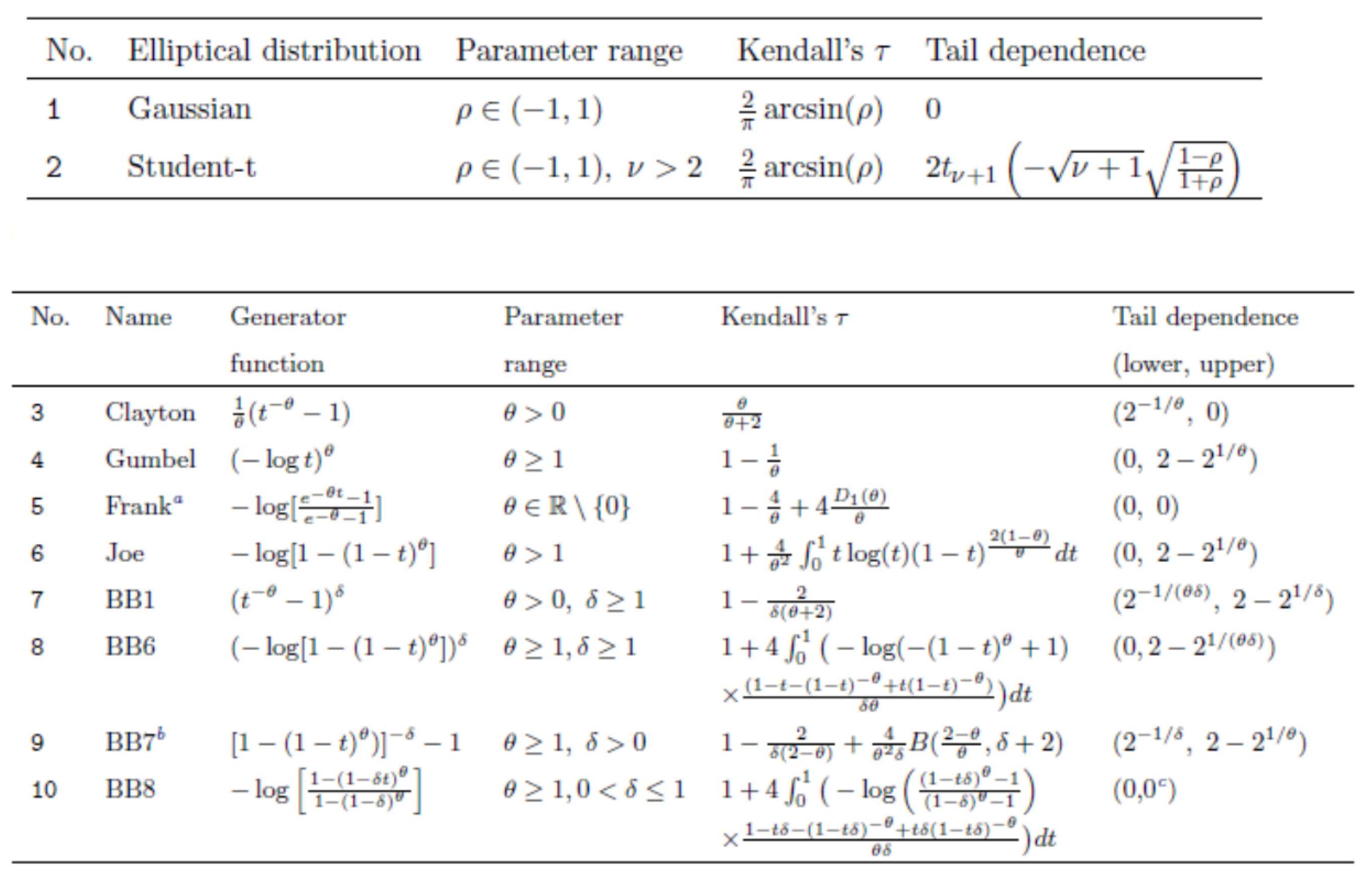
Figure 4.
Example of R-Vine on 4 Variables. (Source Dissman (2010)).

Figure 5.
Matrix Mapping of vine copulas (source Dissman (2010)).

Figure 6.
Use of Matrices to Store R-vine Information (source: Dissman (2010)).
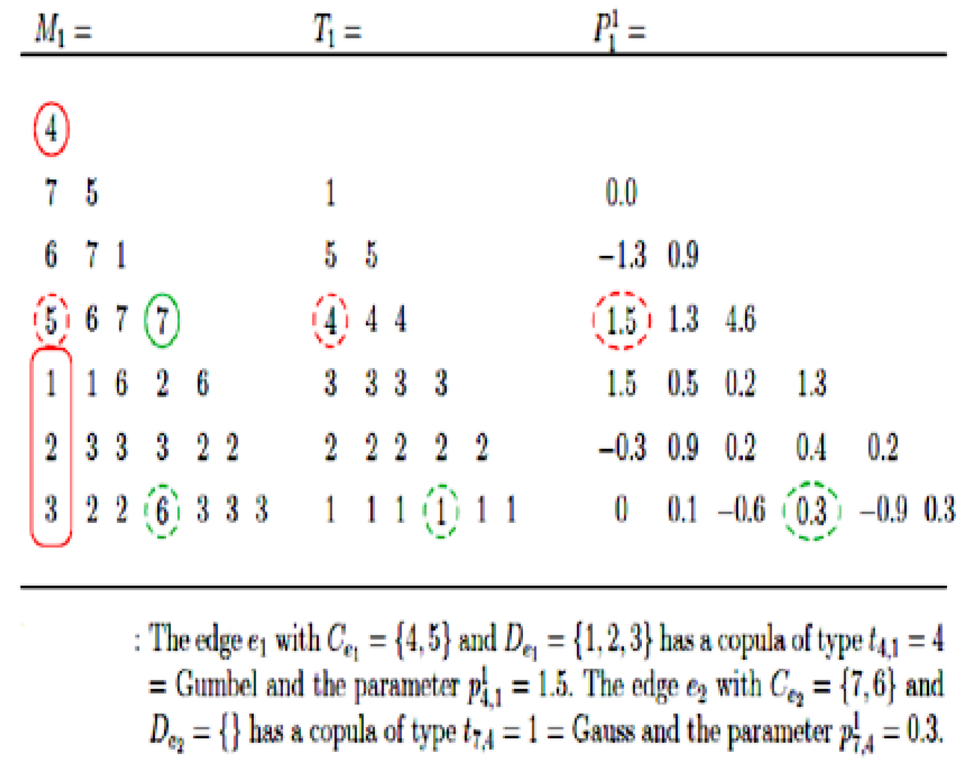
Figure 7.
Results-C-Vine Tree-1 Pre-GFC.

Figure 8.
C-Vine Tree 2 Pre-GFC.

Figure 9.
Results-C-Vine Tree-1 GFC.
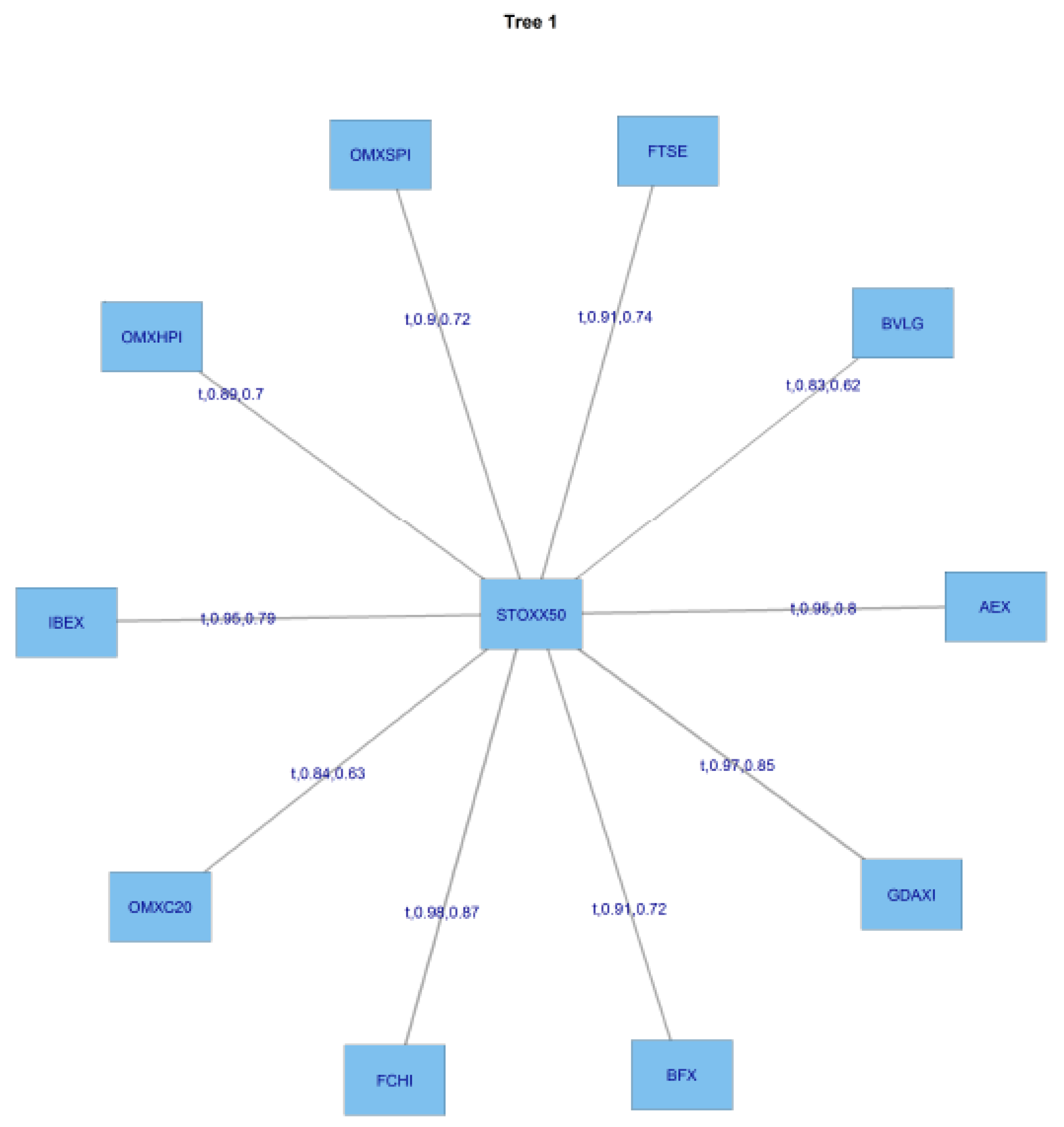
Figure 10.
C-Vine Tree 2 GFC.
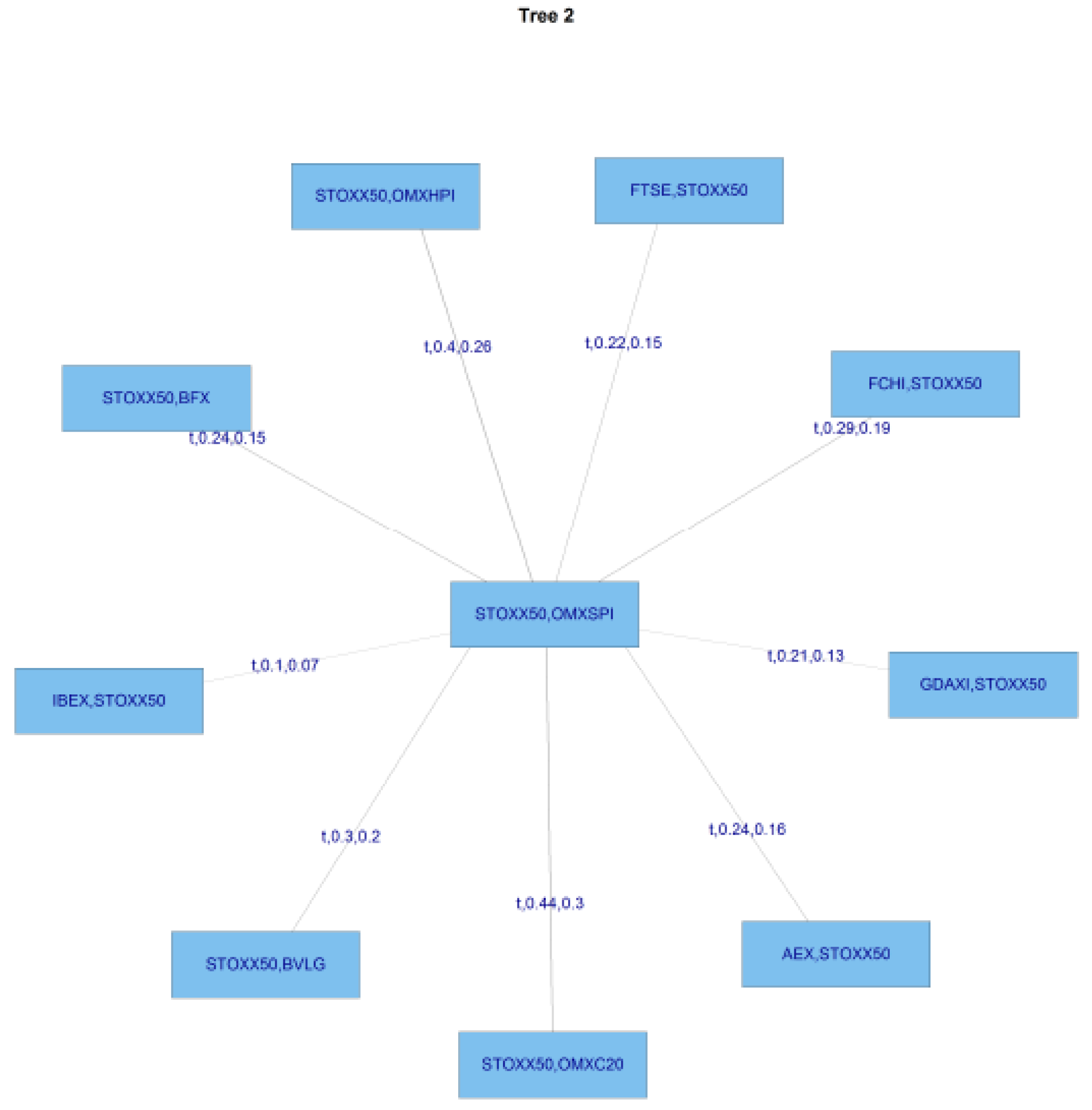
Figure 11.
Results-C-Vine Tree-1 post-GFC.

Figure 12.
Results-C-Vine Tree-2 post-GFC.

Figure 13.
Results-R-Vine Trees-1 and 2 pre-GFC.

Figure 14.
Results-R-Vine Tree-3 pre-GFC.
Figure 15.
Pre-GFC R-Vine Copula Specification Matrix.
Figure 16.
Results-R-Vine Trees-1 and 2 GFC.

Figure 17.
Results-R-Vine Trees-1 and 2 post-GFC.

Figure 18.
Portfolio Value-at-Risk analysis based on application of vine copulas.
Figure 19.
Portfolio Value-at-Risk analysis based on application of a GARCH(1,1) model.


Table 1.
Index Data.
| Reuters RIC Code | Index |
|---|---|
| .FTSE | British FTSE Index |
| .GDAXI | German DAX Index |
| .FCHI | French CAC 40 Index |
| .AEX | AEX Amsterdam Index |
| .IBEX | Spanish Ibex 35 Index |
| .OMXC20 | OMX Copenhagen 20 Index |
| .OMXSPI | OMX Stockholm All Share Index |
| .OMXHPI | OMX Helsinki All Share Index |
| .BVLG | Portuguese PSI General |
| .BFX | Belgian Bell 20 Index |
| .STOXX50 | European STOXX 50 |
Table 2.
Descriptive statistics for indices by sub-period: Pre-GFC, GFC, and Post-GFC.
| Index | PRE-GFC January 2005–June 2007 | GFC July 2007–August 2009 | Post GFC September 2009–December 2013 |
|---|---|---|---|
| .FTSE | |||
| Mean | 0.000555640 | −0.000895714 | 0.000295718 |
| Median | 0.000738054 | 0.000203498 | 0.000584525 |
| St. Deviation | 0.00813613 | 0.0238888 | 0.0129783 |
| Skewness | −0.149519 | 0.0528700 | −0.224389 |
| Ex-Kurtosis | 1.19971 | 4.78545 | 2.23948 |
| Bera-Jarque test | 41.467 (0.00) | 539.38 0.000 | 245.837 (0.00) |
| Hurst Exponent | 41.467 | 0.57554 | 0.453993 |
| .GDAXI | |||
| Mean | 0.000965496 | −0.000573968 | 0.000457927 |
| Median | 0.00117051 | 0.000537208 | 0.000326914 |
| St. Deviation | 0.00984275 | 0.0235477 | 0.0166782 |
| Skewness | −0.198918 | 0.188195 | −0.189233 |
| Ex-Kurtosis | 1.06819 | 4.83638 | 2.14630 |
| Bera-Jarque test | 35.2434 (0.00) | 553.989 (0.00) | 223.835 |
| Hurst exponent | 0.513785 | 0.577037 | 0.503562 |
| .FCHI | |||
| Mean | 0.000704096 | −0.000794553 | 0.000107354 |
| Median | 0.000603012 | 0.000142254 | 0.000167647 |
| St. Deviation | 0.00919530 | 0.0244639 | 0.0178098 |
| Skewness | −0.225337 | 0.187499 | −0.0293812 |
| Ex-Kurtosis | 1.29375 | 4.94817 | 2.75582 |
| Bera-Jarque test | 50.9105 (0.00) | 579.714 (0.00) | 2.75582 |
| Hurst exponent | 0.480051 | 0.570031 | 0.4944 |
| .AEX | |||
| Mean | 0.000706398 | −0.00100306 | 0.000233513 |
| Median | 0.000689552 | 0.000104563 | 0.000746154 |
| St. Deviation | 0.00866571 | 0.0252091 | 0.0151689 |
| Skewness | −0.168285 | 0.0194178 | −0.106574 |
| Ex-Kurtosis | 1.79428 | 4.93931 | 2.18174 |
| Bera-Jarque test | 90.3996 (0.00) | 574.377 (0.00) | 226.455 (0.00) |
| Hurst exponent | 0.510652 | 0.606603 | 0.503613 |
| .IBEX | |||
| Mean | 0.000754932 | −0.000376594 | −0.000156397 |
| Median | 0.000457241 | 0.00000 | 0.000000 |
| St. Deviation | 0.00896277 | 0.0237746 | 0.0199591 |
| Skewness | −0.179712 | 0.0160456 | 0.176078 |
| Ex-Kurtosis | 1.19903 | 4.57761 | 3.89965 |
| Bera-Jarque test | 42.5008 | 493.327 (0.00) | 722.488 (0.00) |
| Hurst exponent | 0.51974 | 0.602261 | 0.552881 |
| .OMXC20 | |||
| Mean | 0.000812167 | −0.000564910 | 0.000499859 |
| Median | 0.00132764 | 0.00000 | 0.000802048 |
| St. Deviation | 0.00993412 | 0.0239638 | 0.0144641 |
| Skewness | −0.765524 | −0.187144 | −0.116423 |
| Ex-Kurtosis | 2.80674 | 4.22380 | 2.12358 |
| Bera-Jarque test | 277.268 (0.00) | 423.095 (0.00) | 215.069 |
| Hurst exponent | 0.498681 | 0.59553 | 0.520375 |
Table 3.
Descriptive statistics for indices by sub-period: Pre-GFC, GFC, and Post-GFC (Contd).
| Index | PRE-GFC January 2005–June 2007 | GFC July 2007–August 2009 | Post GFC September 2009–December 2013 |
|---|---|---|---|
| .OMXSPI | |||
| Mean | 0.000865551 | −0.000760510 | 0.000458071 |
| Median | 0.000980873 | 0.00000 | 0.000724200 |
| St. Deviation | 0.0111512 | 0.0276237 | 0.0177400 |
| Skewness | −0.295747 | 0.230350 | −0.208441 |
| Ex-Kurtosis | 3.58218 | 2.34544 | 2.67172 |
| Bera-Jarque test | 357.559 | 134.501 (0.00) | 344.573 (0.00) |
| Hurst exponent | 0.522449 | 0.574409 | 0.497336 |
| .OMXHPI | |||
| Mean | 0.000938877 | −0.000984965 | 0.000108658 |
| Median | 0.000484177 | −0.000943853 | 0.000373821 |
| St. Deviation | 0.0103049 | 0.0242644 | 0.0167601 |
| Skewness | −0.115052 | 0.139482 | −0.115636 |
| Ex-Kurtosis | 2.36500 | 2.40933 | 2.21433 |
| Bera-Jarque test | 153.152 | 138.489 | 233.587 (0.00) |
| Hurst exponent | 0.49008 | 0.61372 | 0.538587 |
| .BVLG | |||
| Mean | 0.000891032 | −0.000884323 | −0.000169933 |
| Median | 0.000892271 | −8.71710e-005 | 5.77024e-005 |
| St. Deviation | 0.00703327 | 0.0199733 | 0.0159551 |
| Skewness | 0.0898224 | −0.160906 | −0.00138346 |
| Ex-Kurtosis | 1.05671 | 6.43503 | 3.74001 |
| Bera-Jarque test | 31.64 (0.01) | 977.29 (0.00) | 659.168 (0.00) |
| Hurst exponent | 0.6217 | 0.614598 | 0.556314 |
| .BFX | |||
| Mean | 0.000692830 | −0.00108296 | 0.000151703 |
| Median | 0.000817080 | 0.00000 | 0.000179149 |
| St. Deviation | 0.00877648 | 0.0222434 | 0.0158848 |
| Skewness | −0.225903 | −0.131889 | 0.00987544 |
| Ex-Kurtosis | 1.59909 | 3.23142 | 2.90360 |
| Bera-Jarque test | 74.898 | 247.462 (0.00) | 397.323 (0.00) |
| Hurst exponent | 0.54556 | 0.641453 | 0.497547 |
| .STOXX50 | |||
| Mean | 0.000642054 | −0.000752410 | 6.45717e-005 |
| Median | 0.000635064 | 0.000153018 | 0.00000 |
| St. Deviation | 0.00922232 | 0.0241936 | 0.0179815 |
| Skewness | −0.154465 | 0.0851528 | 0.00350895 |
| Ex-Kurtosis | 1.33626 | 4.29802 | 2.88743 |
| Bera-Jarque test | 51.0231 (0.00) | 435.568 (0.00) | 392.895 (0.00) |
| Hurst exponent | 0.474577 | 0.587196 | 0.504895 |
Table 4.
Pre-GFC C-Vine Copula Structure.
| FTSE | GDAXI | FCHI | AEX | IBEX | STOXX50 | OMXC20 | OMXSPI | OMXHPI | BVLG | BFX | |
|---|---|---|---|---|---|---|---|---|---|---|---|
| FTSE | 1 | 0 | 0 | 0 | 0 | 0 | 0 | 0 | 0 | 0 | 0 |
| GDAXI | 9 | 3 | 0 | 0 | 0 | 0 | 0 | 0 | 0 | 0 | 0 |
| FCHI | 3 | 9 | 9 | 0 | 0 | 0 | 0 | 0 | 0 | 0 | 0 |
| AEX | 10 | 10 | 10 | 2 | 0 | 0 | 0 | 0 | 0 | 0 | 0 |
| IBEX | 2 | 2 | 2 | 10 | 4 | 0 | 0 | 0 | 0 | 0 | 0 |
| STOXX50 | 4 | 4 | 4 | 4 | 10 | 5 | 0 | 0 | 0 | 0 | 0 |
| OMXC20 | 5 | 5 | 5 | 5 | 5 | 10 | 7 | 0 | 0 | 0 | 0 |
| OMXSPI | 7 | 7 | 7 | 7 | 7 | 7 | 10 | 8 | 0 | 0 | 0 |
| OMXHPI | 8 | 8 | 8 | 8 | 8 | 8 | 8 | 10 | 10 | 0 | 0 |
| BVLG | 11 | 11 | 11 | 11 | 11 | 11 | 11 | 11 | 11 | 11 | 0 |
| BFX | 6 | 6 | 6 | 6 | 6 | 6 | 6 | 6 | 6 | 6 | 6 |
Table 5.
Pre-GFC C-Vine Copula Specification Matrix.
| FTSE | GDAXI | FCHI | AEX | IBEX | STOXX50 | OMXC20 | OMXSPI | OMXHPI | BVLG | BFX | |
|---|---|---|---|---|---|---|---|---|---|---|---|
| FTSE | 0 | 0 | 0 | 0 | 0 | 0 | 0 | 0 | 0 | 0 | 0 |
| GDAXI | 2 | 0 | 0 | 0 | 0 | 0 | 0 | 0 | 0 | 0 | 0 |
| FCHI | 2 | 2 | 0 | 0 | 0 | 0 | 0 | 0 | 0 | 0 | 0 |
| AEX | 2 | 3 | 5 | 0 | 0 | 0 | 0 | 0 | 0 | 0 | 0 |
| IBEX | 5 | 2 | 2 | 1 | 0 | 0 | 0 | 0 | 0 | 0 | 0 |
| STOXX50 | 5 | 2 | 1 | 5 | 5 | 0 | 0 | 0 | 0 | 0 | 0 |
| OMXC20 | 3 | 2 | 3 | 1 | 1 | 1 | 0 | 0 | 0 | 0 | 0 |
| OMXSPI | 5 | 1 | 5 | 5 | 3 | 4 | 5 | 0 | 0 | 0 | 0 |
| OMXHPI | 1 | 3 | 2 | 3 | 6 | 5 | 1 | 5 | 0 | 0 | 0 |
| BVLG | 5 | 1 | 5 | 5 | 5 | 2 | 1 | 3 | 1 | 0 | 0 |
| BFX | 2 | 2 | 2 | 2 | 2 | 2 | 2 | 2 | 2 | 2 | 0 |
Table 6.
Pre-GFC C-Vine Copula Parameter Estimates.
| FTSE | GDAXI | FCHI | AEX | IBEX | STOXX50 | OMXC20 | OMXSPI | OMXHPI | BVLG | BFX | |
|---|---|---|---|---|---|---|---|---|---|---|---|
| FTSE | 0 | 0 | 0 | 0 | 0 | 0 | 0 | 0 | 0 | 0 | 0 |
| GDAXI | 0.152236 | 0 | 0 | 0 | 0 | 0 | 0 | 0 | 0 | 0 | 0 |
| FCHI | 0.786802 | 0.437083 | 0 | 0 | 0 | 0 | 0 | 0 | 0 | 0 | 0 |
| AEX | 1.418514 | 0.053894 | 1.036334 | 0 | 0 | 0 | 0 | 0 | 0 | 0 | 0 |
| IBEX | 1.033914 | 0.672986 | 0.162141 | 0.137522 | 0 | 0 | 0 | 0 | 0 | 0 | 0 |
| STOXX50 | −0.18660 | 1.068144 | 0.155770 | 0.076751 | 0.205075 | 0 | 0 | 0 | 0 | 0 | 0 |
| OMXC20 | −0.06799 | −0.011583 | −0.092367 | 0.201391 | 0.973316 | 0.083272 | 0 | 0 | 0 | 0 | 0 |
| OMXSPI | −0.16274 | 0.016648 | −0.261361 | 0.182827 | 0.714802 | 0.047323 | −0.025852 | 0 | 0 | 0 | 0 |
| OMXHPI | 1.05367 | 0.087220 | 0.0779183 | 0.126660 | 0.071290 | −0.004308 | 0.031866 | 1.223109 | 0 | 0 | 0 |
| BVLG | 1.56654 | 0.164849 | 1.2442506 | 0.408728 | −0.130783 | −0.129392 | 0.148569 | 0.226344 | 0.196334 | 0 | 0 |
| BFX | 0.94972 | 0.871079 | 0.9334080 | 0.8309762 | 0.827286 | 0.973728 | 0.978593 | 0.693275 | 0.890633 | 0.718538 | 0 |
Table 7.
Pre-GFC C-Vine Copula Second Parameter Estimates.
| FTSE | GDAXI | FCHI | AEX | IBEX | STOXX50 | OMXC20 | OMXSPI | OMXHPI | BVLG | BFX | |
|---|---|---|---|---|---|---|---|---|---|---|---|
| FTSE | 0 | 0 | 0 | 0 | 0 | 0 | 0 | 0 | 0 | 0 | 0 |
| GDAXI | 15.375671 | 0 | 0 | 0 | 0 | 0 | 0 | 0 | 0 | 0 | 0 |
| FCHI | 9.544367 | 12.310803 | 0 | 0 | 0 | 0 | 0 | 0 | 0 | 0 | 0 |
| AEX | 9.401744 | 0 | 0 | 0 | 0 | 0 | 0 | 0 | 0 | 0 | 0 |
| IBEX | 0 | 10.267206 | 10.233424 | 0 | 0 | 0 | 0 | 0 | 0 | 0 | 0 |
| STOXX50 | 0 | 10.124756 | 0 | 0 | 0 | 0 | 0 | 0 | 0 | 0 | 0 |
| OMXC20 | 0 | 8.646548 | 0 | 0 | 0 | 0 | 0 | 0 | 0 | 0 | 0 |
| OMXSPI | 0 | 0 | 0 | 0 | 0 | 0 | 0 | 0 | 0 | 0 | 0 |
| OMXHPI | 0 | 0 | 8.390870 | 0 | 0 | 0 | 0 | 0 | 0 | 0 | 0 |
| BVLG | 0 | 0 | 0 | 0 | 0 | 12.429237 | 0 | 0 | 0 | 0 | 0 |
| BFX | 8.686229 | 5.378347 | 3.377834 | 8.575454 | 11.885624 | 7.882211 | 6.454538 | 9.626281 | 13.482133 | 8.332783 | 0 |
Table 8.
Pre-GFC C-Vine Copula Tau matrix.
| FTSE | GDAXI | FCHI | AEX | IBEX | STOXX50 | OMXC20 | OMXSPI | OMXHPI | BVLG | BFX | |
|---|---|---|---|---|---|---|---|---|---|---|---|
| FTSE | 0.000000 | 0.000000 | 0.000000 | 0.000000 | 0.000000 | 0.000000 | 0.000000 | 0.000000 | 0.000000 | 0.000000 | 0.000000 |
| GDAXI | 0.004067 | 0.000000 | 0.000000 | 0.000000 | 0.000000 | 0.000000 | 0.000000 | 0.000000 | 0.000000 | 0.000000 | 0.000000 |
| FCHI | 0.036096 | −0.029548 | 0.000000 | 0.000000 | 0.000000 | 0.000000 | 0.000000 | 0.000000 | 0.000000 | 0.000000 | 0.000000 |
| AEX | 0.014419 | 0.030447 | 0.068843 | 0.000000 | 0.000000 | 0.000000 | 0.000000 | 0.000000 | 0.000000 | 0.000000 | 0.000000 |
| IBEX | 0.005771 | −0.091656 | −0.099620 | 0.025585 | 0.000000 | 0.000000 | 0.000000 | 0.000000 | 0.000000 | 0.000000 | 0.000000 |
| STOXX50 | 0.155059 | −0.031242 | −0.053529 | −0.007041 | 0.075579 | 0.000000 | 0.000000 | 0.000000 | 0.000000 | 0.000000 | 0.000000 |
| OMXC20 | 0.036919 | −0.085254 | 0.030712 | −0.029132 | −0.109944 | 0.101804 | 0.000000 | 0.000000 | 0.000000 | 0.000000 | 0.000000 |
| OMXSPI | 0.062762 | 0.067815 | 0.106788 | −0.007854 | 0.069387 | 0.037842 | 0.118612 | 0.000000 | 0.000000 | 0.000000 | 0.000000 |
| OMXHPI | 0.084060 | 0.056764 | 0.258504 | 0.035254 | 0.039828 | 0.116247 | 0.152900 | 0.096636 | 0.000000 | 0.000000 | 0.000000 |
| BVLG | 0.121015 | 0.168311 | 0.082120 | −0.024858 | 0.162175 | 0.101571 | 0.173707 | 0.120451 | 0.224388 | 0.000000 | 0.000000 |
| BFX | 0.673160 | 0.868040 | 0.620234 | 0.853751 | 0.797280 | 0.766361 | 0.478690 | 0.624435 | 0.472402 | 0.692177 | 0.000000 |
Table 9.
GFC C-Vine Copula Structure.
| FTSE | GDAXI | FCHI | AEX | IBEX | STOXX50 | OMXC20 | OMXSPI | OMXHPI | BVLG | BFX | |
|---|---|---|---|---|---|---|---|---|---|---|---|
| FTSE | 1 | 0 | 0 | 0 | 0 | 0 | 0 | 0 | 0 | 0 | 0 |
| GDAXI | 9 | 9 | 0 | 0 | 0 | 0 | 0 | 0 | 0 | 0 | 0 |
| FCHI | 11 | 11 | 5 | 0 | 0 | 0 | 0 | 0 | 0 | 0 | 0 |
| AEX | 5 | 5 | 11 | 2 | 0 | 0 | 0 | 0 | 0 | 0 | 0 |
| IBEX | 2 | 2 | 2 | 11 | 10 | 0 | 0 | 0 | 0 | 0 | 0 |
| STOXX50 | 10 | 10 | 10 | 10 | 11 | 3 | 0 | 0 | 0 | 0 | 0 |
| OMXC20 | 3 | 3 | 3 | 3 | 3 | 11 | 4 | 0 | 0 | 0 | 0 |
| OMXSPI | 4 | 4 | 4 | 4 | 4 | 4 | 11 | 7 | 0 | 0 | 0 |
| OMXHPI | 7 | 7 | 7 | 7 | 7 | 7 | 7 | 11 | 8 | 0 | 0 |
| BVLG | 8 | 8 | 8 | 8 | 8 | 8 | 8 | 8 | 11 | 11 | 0 |
| BFX | 6 | 6 | 6 | 6 | 6 | 6 | 6 | 6 | 6 | 6 | 6 |
Table 10.
GFC C-Vine Copula Specification Matrix.
| FTSE | GDAXI | FCHI | AEX | IBEX | STOXX50 | OMXC20 | OMXSPI | OMXHPI | BVLG | BFX | |
|---|---|---|---|---|---|---|---|---|---|---|---|
| FTSE | 0 | 0 | 0 | 0 | 0 | 0 | 0 | 0 | 0 | 0 | 0 |
| GDAXI | 6 | 0 | 0 | 0 | 0 | 0 | 0 | 0 | 0 | 0 | 0 |
| FCHI | 2 | 2 | 0 | 0 | 0 | 0 | 0 | 0 | 0 | 0 | 0 |
| AEX | 3 | 1 | 5 | 0 | 0 | 0 | 0 | 0 | 0 | 0 | 0 |
| IBEX | 1 | 2 | 2 | 2 | 0 | 0 | 0 | 0 | 0 | 0 | 0 |
| STOXX50 | 5 | 3 | 4 | 5 | 2 | 0 | 0 | 0 | 0 | 0 | 0 |
| OMXC20 | 5 | 2 | 6 | 4 | 2 | 4 | 0 | 0 | 0 | 0 | 0 |
| OMXSPI | 2 | 2 | 2 | 2 | 2 | 2 | 2 | 0 | 0 | 0 | 0 |
| OMXHPI | 1 | 4 | 2 | 2 | 5 | 2 | 2 | 5 | 0 | 0 | 0 |
| BVLG | 2 | 2 | 2 | 2 | 2 | 2 | 2 | 2 | 2 | 0 | 0 |
| BFX | 2 | 2 | 2 | 2 | 2 | 2 | 2 | 2 | 2 | 2 | 0 |
Table 11.
GFC C-Vine Copula Tau matrix.
| FTSE | GDAXI | FCHI | AEX | IBEX | STOXX50 | OMXC20 | OMXSPI | OMXHPI | BVLG | BFX | |
|---|---|---|---|---|---|---|---|---|---|---|---|
| FTSE | 0.000000 | 0.000000 | 0.000000 | 0.000000 | 0.000000 | 0.000000 | 0.000000 | 0.000000 | 0.000000 | 0.000000 | 0.000000 |
| GDAXI | 0.015375 | 0.000000 | 0.000000 | 0.000000 | 0.000000 | 0.000000 | 0.000000 | 0.000000 | 0.000000 | 0.000000 | 0.000000 |
| FCHI | −0.014081 | −0.039582 | 0.000000 | 0.000000 | 0.000000 | 0.000000 | 0.000000 | 0.000000 | 0.000000 | 0.000000 | 0.000000 |
| AEX | 0.056810 | −0.066848 | −0.006416 | 0.000000 | 0.000000 | 0.000000 | 0.000000 | 0.000000 | 0.000000 | 0.000000 | 0.000000 |
| IBEX | −0.025651 | −0.042298 | −0.058784 | −0.083306 | 0.000000 | 0.000000 | 0.000000 | 0.000000 | 0.000000 | 0.000000 | 0.000000 |
| STOXX50 | 0.036874 | 0.051407 | 0.139010 | −0.030941 | 0.108496 | 0.000000 | 0.000000 | 0.000000 | 0.000000 | 0.000000 | 0.000000 |
| OMXC20 | 0.153082 | 0.015462 | 0.035938 | 0.124012 | −0.006829 | 0.041608 | 0.000000 | 0.000000 | 0.000000 | 0.000000 | 0.000000 |
| OMXSPI | 0.131300 | 0.032328 | −0.067132 | −0.064857 | 0.029947 | 0.132041 | 0.162546 | 0.000000 | 0.000000 | 0.000000 | 0.000000 |
| OMXHPI | 0.124725 | 0.124603 | 0.080170 | 0.011683 | 0.194322 | 0.106381 | 0.103593 | 0.126699 | 0.000000 | 0.000000 | 0.000000 |
| BVLG | 0.143013 | 0.264481 | 0.064391 | 0.133197 | 0.195961 | 0.189751 | 0.154686 | 0.292464 | 0.153108 | 0.000000 | 0.000000 |
| BFX | 0.735492 | 0.702116 | 0.790637 | 0.844666 | 0.625231 | 0.867456 | 0.801941 | 0.630802 | 0.718425 | 0.720695 | 0.000000 |
Table 12.
Post-GFC C-Vine Copula Structure.
| FTSE | GDAXI | FCHI | AEX | IBEX | STOXX50 | OMXC20 | OMXSPI | OMXHPI | BVLG | BFX | |
|---|---|---|---|---|---|---|---|---|---|---|---|
| FTSE | 2 | 0 | 0 | 0 | 0 | 0 | 0 | 0 | 0 | 0 | 0 |
| GDAXI | 11 | 7 | 0 | 0 | 0 | 0 | 0 | 0 | 0 | 0 | 0 |
| FCHI | 7 | 11 | 1 | 0 | 0 | 0 | 0 | 0 | 0 | 0 | 0 |
| AEX | 1 | 1 | 11 | 3 | 0 | 0 | 0 | 0 | 0 | 0 | 0 |
| IBEX | 3 | 3 | 3 | 11 | 9 | 0 | 0 | 0 | 0 | 0 | 0 |
| STOXX50 | 9 | 9 | 9 | 9 | 11 | 10 | 0 | 0 | 0 | 0 | 0 |
| OMXC20 | 10 | 10 | 10 | 10 | 10 | 11 | 5 | 0 | 0 | 0 | 0 |
| OMXSPI | 5 | 5 | 5 | 5 | 5 | 5 | 11 | 8 | 0 | 0 | 0 |
| OMXHPI | 8 | 8 | 8 | 8 | 8 | 8 | 8 | 11 | 4 | 0 | 0 |
| BVLG | 4 | 4 | 4 | 4 | 4 | 4 | 4 | 4 | 11 | 11 | 0 |
| BFX | 6 | 6 | 6 | 6 | 6 | 6 | 6 | 6 | 6 | 6 | 6 |
Table 13.
Post-GFC C-Vine Copula Specification Matrix.
| FTSE | GDAXI | FCHI | AEX | IBEX | STOXX50 | OMXC20 | OMXSPI | OMXHPI | BVLG | BFX | |
|---|---|---|---|---|---|---|---|---|---|---|---|
| FTSE | 0 | 0 | 0 | 0 | 0 | 0 | 0 | 0 | 0 | 0 | 0 |
| GDAXI | 3 | 0 | 0 | 0 | 0 | 0 | 0 | 0 | 0 | 0 | 0 |
| FCHI | 1 | 3 | 0 | 0 | 0 | 0 | 0 | 0 | 0 | 0 | 0 |
| AEX | 3 | 1 | 4 | 0 | 0 | 0 | 0 | 0 | 0 | 0 | 0 |
| IBEX | 2 | 4 | 2 | 3 | 0 | 0 | 0 | 0 | 0 | 0 | 0 |
| STOXX50 | 3 | 5 | 1 | 5 | 4 | 0 | 0 | 0 | 0 | 0 | 0 |
| OMXC20 | 3 | 4 | 1 | 1 | 4 | 2 | 0 | 0 | 0 | 0 | 0 |
| OMXSPI | 2 | 2 | 5 | 2 | 1 | 1 | 3 | 0 | 0 | 0 | 0 |
| OMXHPI | 4 | 2 | 2 | 1 | 2 | 5 | 5 | 1 | 0 | 0 | 0 |
| BVLG | 3 | 2 | 2 | 2 | 2 | 6 | 1 | 1 | 2 | 0 | 0 |
| BFX | 2 | 2 | 2 | 2 | 2 | 2 | 2 | 2 | 2 | 2 | 0 |
Table 14.
Post-GFC C-Vine Copula Tau matrix.
| FTSE | GDAXI | FCHI | AEX | IBEX | STOXX50 | OMXC20 | OMXSPI | OMXHPI | BVLG | BFX | |
|---|---|---|---|---|---|---|---|---|---|---|---|
| FTSE | 0.000000 | 0.000000 | 0.000000 | 0.000000 | 0.000000 | 0.000000 | 0.000000 | 0.000000 | 0.000000 | 0.000000 | 0.000000 |
| GDAXI | 0.016107 | 0.000000 | 0.000000 | 0.000000 | 0.000000 | 0.000000 | 0.000000 | 0.000000 | 0.000000 | 0.000000 | 0.000000 |
| FCHI | 0.036144 | 0.035753 | 0.000000 | 0.000000 | 0.000000 | 0.000000 | 0.000000 | 0.000000 | 0.000000 | 0.000000 | 0.000000 |
| AEX | 0.052784 | 0.024838 | 0.031775 | 0.000000 | 0.000000 | 0.000000 | 0.000000 | 0.000000 | 0.000000 | 0.000000 | 0.000000 |
| IBEX | −0.130688 | 0.044635 | 0.051311 | 0.046822 | 0.000000 | 0.000000 | 0.000000 | 0.000000 | 0.000000 | 0.000000 | 0.000000 |
| STOXX50 | 0.047183 | 0.135747 | −0.023586 | −0.027756 | 0.086703 | 0.000000 | 0.000000 | 0.000000 | 0.000000 | 0.000000 | 0.000000 |
| OMXC20 | 0.017433 | 0.131760 | −0.035346 | 0.042679 | 0.088264 | 0.198073 | 0.000000 | 0.000000 | 0.000000 | 0.000000 | 0.000000 |
| OMXSPI | −0.264456 | −0.021457 | −0.078220 | −0.228646 | 0.003425 | 0.202873 | 0.059906 | 0.000000 | 0.000000 | 0.000000 | 0.000000 |
| OMXHPI | 0.118687 | 0.228880 | 0.072495 | 0.108799 | 0.324425 | 0.072847 | −0.019366 | 0.131302 | 0.000000 | 0.000000 | 0.000000 |
| BVLG | 0.142026 | 0.226714 | 0.302870 | 0.255696 | 0.209531 | 0.019685 | −0.207497 | 0.284246 | 0.239010 | 0.000000 | 0.000000 |
| BFX | 0.856993 | 0.629740 | 0.718863 | 0.912498 | 0.736706 | 0.707156 | 0.819042 | 0.721526 | 0.847664 | 0.818948 | 0.000000 |
Table 15.
Pre-GFC R-Vine Copula Structure.
| FTSE | GDAXI | FCHI | AEX | IBEX | STOXX50 | OMXC20 | OMXSPI | OMXHPI | BVLG | BFX | |
|---|---|---|---|---|---|---|---|---|---|---|---|
| FTSE | 4 | 0 | 0 | 0 | 0 | 0 | 0 | 0 | 0 | 0 | 0 |
| GDAXI | 7 | 1 | 0 | 0 | 0 | 0 | 0 | 0 | 0 | 0 | 0 |
| FCHI | 10 | 7 | 5 | 0 | 0 | 0 | 0 | 0 | 0 | 0 | 0 |
| AEX | 11 | 10 | 7 | 8 | 0 | 0 | 0 | 0 | 0 | 0 | 0 |
| IBEX | 3 | 11 | 10 | 7 | 9 | 0 | 0 | 0 | 0 | 0 | 0 |
| STOXX50 | 2 | 3 | 11 | 10 | 7 | 2 | 0 | 0 | 0 | 0 | 0 |
| OMXC20 | 9 | 2 | 3 | 11 | 10 | 7 | 6 | 0 | 0 | 0 | 0 |
| OMXSPI | 5 | 9 | 2 | 3 | 11 | 10 | 7 | 7 | 0 | 0 | 0 |
| OMXHPI | 8 | 5 | 9 | 2 | 3 | 11 | 10 | 10 | 3 | 0 | 0 |
| BVLG | 1 | 8 | 8 | 9 | 2 | 3 | 11 | 11 | 10 | 11 | 0 |
| BFX | 6 | 6 | 6 | 6 | 6 | 6 | 3 | 3 | 11 | 10 | 10 |
Table 16.
Pre-GFC R-Vine Copula Tau matrix.
| FTSE | GDAXI | FCHI | AEX | IBEX | STOXX50 | OMXC20 | OMXSPI | OMXHPI | BVLG | BFX | |
|---|---|---|---|---|---|---|---|---|---|---|---|
| FTSE | 0.000000 | 0.000000 | 0.000000 | 0.000000 | 0.000000 | 0.000000 | 0.000000 | 0.000000 | 0.000000 | 0.000000 | 0.000000 |
| GDAXI | 0.070734 | 0.000000 | 0.000000 | 0.000000 | 0.000000 | 0.000000 | 0.000000 | 0.000000 | 0.000000 | 0.000000 | 0.000000 |
| FCHI | 0.086887 | 0.048472 | 0.000000 | 0.000000 | 0.000000 | 0.000000 | 0.000000 | 0.000000 | 0.000000 | 0.000000 | 0.000000 |
| AEX | 0.154546 | 0.034327 | 0.035060 | 0.000000 | 0.000000 | 0.000000 | 0.000000 | 0.000000 | 0.000000 | 0.000000 | 0.000000 |
| IBEX | 0.019231 | 0.074440 | 0.103680 | 0.087828 | 0.000000 | 0.000000 | 0.000000 | 0.000000 | 0.000000 | 0.000000 | 0.000000 |
| STOXX50 | −0.020726 | 0.063797 | 0.099572 | 0.036958 | 0.131488 | 0.000000 | 0.000000 | 0.000000 | 0.000000 | 0.000000 | 0.000000 |
| OMXC20 | −0.043319 | −0.007375 | −0.058887 | 0.091484 | 0.107138 | 0.009252 | 0.000000 | 0.000000 | 0.000000 | 0.000000 | 0.000000 |
| OMXSPI | −0.104071 | 0.010599 | −0.029020 | 0.083757 | 0.079020 | 0.030138 | −0.016460 | 0.000000 | 0.000000 | 0.000000 | 0.000000 |
| OMXHPI | 0.050943 | 0.055597 | 0.037498 | 0.059558 | 0.034418 | −0.002743 | 0.015683 | 0.133918 | 0.000000 | 0.000000 | 0.000000 |
| BVLG | 0.169959 | 0.105428 | 0.136164 | 0.268055 | −0.083498 | −0.082605 | 0.094934 | 0.145355 | 0.089392 | 0.000000 | 0.000000 |
| BFX | 0.797280 | 0.673160 | 0.766361 | 0.624435 | 0.620234 | 0.853751 | 0.868040 | 0.487667 | 0.699477 | 0.510377 | 0.000000 |
Table 17.
GFC R-Vine Copula Specification Matrix.
| FTSE | GDAXI | FCHI | AEX | IBEX | STOXX50 | OMXC20 | OMXSPI | OMXHPI | BVLG | BFX | |
|---|---|---|---|---|---|---|---|---|---|---|---|
| FTSE | 0 | 0 | 0 | 0 | 0 | 0 | 0 | 0 | 0 | 0 | 0 |
| GDAXI | 3 | 0 | 0 | 0 | 0 | 0 | 0 | 0 | 0 | 0 | 0 |
| FCHI | 2 | 2 | 0 | 0 | 0 | 0 | 0 | 0 | 0 | 0 | 0 |
| AEX | 4 | 1 | 2 | 0 | 0 | 0 | 0 | 0 | 0 | 0 | 0 |
| IBEX | 5 | 5 | 2 | 2 | 0 | 0 | 0 | 0 | 0 | 0 | 0 |
| STOXX50 | 3 | 2 | 1 | 6 | 4 | 0 | 0 | 0 | 0 | 0 | 0 |
| OMXC20 | 2 | 1 | 2 | 5 | 2 | 2 | 0 | 0 | 0 | 0 | 0 |
| OMXSPI | 1 | 2 | 4 | 2 | 4 | 2 | 2 | 0 | 0 | 0 | 0 |
| OMXHPI | 5 | 2 | 2 | 2 | 2 | 2 | 2 | 2 | 0 | 0 | 0 |
| BVLG | 2 | 2 | 2 | 2 | 2 | 2 | 2 | 4 | 2 | 0 | 0 |
| BFX | 2 | 2 | 2 | 2 | 2 | 2 | 2 | 2 | 2 | 2 | 0 |
Table 18.
GFC R-Vine Copula Tau matrix.
| FTSE | GDAXI | FCHI | AEX | IBEX | STOXX50 | OMXC20 | OMXSPI | OMXHPI | BVLG | BFX | |
|---|---|---|---|---|---|---|---|---|---|---|---|
| FTSE | 0.000000 | 0.000000 | 0.000000 | 0.000000 | 0.000000 | 0.000000 | 0.000000 | 0.000000 | 0.000000 | 0.000000 | 0.000000 |
| GDAXI | 0.020428 | 0.000000 | 0.000000 | 0.000000 | 0.000000 | 0.000000 | 0.000000 | 0.000000 | 0.000000 | 0.000000 | 0.000000 |
| FCHI | 0.040243 | −0.050241 | 0.000000 | 0.000000 | 0.000000 | 0.000000 | 0.000000 | 0.000000 | 0.000000 | 0.000000 | 0.000000 |
| AEX | 0.090111 | −0.051601 | 0.034037 | 0.000000 | 0.000000 | 0.000000 | 0.000000 | 0.000000 | 0.000000 | 0.000000 | 0.000000 |
| IBEX | 0.174882 | −0.023305 | 0.201117 | 0.060031 | 0.000000 | 0.000000 | 0.000000 | 0.000000 | 0.000000 | 0.000000 | 0.000000 |
| STOXX50 | 0.085350 | 0.133903 | 0.134654 | 0.037200 | 0.047610 | 0.000000 | 0.000000 | 0.000000 | 0.000000 | 0.000000 | 0.000000 |
| OMXC20 | 0.074012 | −0.026941 | 0.088942 | 0.067369 | 0.074824 | −0.048008 | 0.000000 | 0.000000 | 0.000000 | 0.000000 | 0.000000 |
| OMXSPI | −0.020369 | -0.069500 | 0.087310 | 0.014613 | 0.038448 | 0.063628 | −0.004543 | 0.000000 | 0.000000 | 0.000000 | 0.000000 |
| OMXHPI | 0.106049 | −0.070206 | 0.093532 | 0.133080 | 0.076088 | 0.052608 | −0.033877 | 0.031725 | 0.000000 | 0.000000 | 0.000000 |
| BVLG | 0.203436 | 0.147673 | 0.112357 | 0.125506 | 0.176601 | 0.208258 | 0.177847 | 0.135507 | 0.183817 | 0.000000 | 0.000000 |
| BFX | 0.651592 | 0.844666 | 0.725372 | 0.749098 | 0.867456 | 0.801941 | 0.790637 | 0.702116 | 0.625231 | 0.720695 | 0.000000 |
Table 19.
Post-GFC R-Vine Copula Specification Matrix.
| FTSE | GDAXI | FCHI | AEX | IBEX | STOXX50 | OMXC20 | OMXSPI | OMXHPI | BVLG | BFX | |
|---|---|---|---|---|---|---|---|---|---|---|---|
| FTSE | 0 | 0 | 0 | 0 | 0 | 0 | 0 | 0 | 0 | 0 | 0 |
| GDAXI | 6 | 0 | 0 | 0 | 0 | 0 | 0 | 0 | 0 | 0 | 0 |
| FCHI | 2 | 3 | 0 | 0 | 0 | 0 | 0 | 0 | 0 | 0 | 0 |
| AEX | 5 | 5 | 4 | 0 | 0 | 0 | 0 | 0 | 0 | 0 | 0 |
| IBEX | 1 | 5 | 5 | 2 | 0 | 0 | 0 | 0 | 0 | 0 | 0 |
| STOXX50 | 1 | 6 | 5 | 1 | 1 | 0 | 0 | 0 | 0 | 0 | 0 |
| OMXC20 | 3 | 5 | 3 | 6 | 3 | 1 | 0 | 0 | 0 | 0 | 0 |
| OMXSPI | 6 | 2 | 1 | 4 | 5 | 3 | 1 | 0 | 0 | 0 | 0 |
| OMXHPI | 5 | 1 | 5 | 2 | 2 | 1 | 2 | 2 | 0 | 0 | 0 |
| BVLG | 2 | 2 | 2 | 5 | 2 | 2 | 2 | 2 | 2 | 0 | 0 |
| BFX | 2 | 2 | 2 | 2 | 2 | 2 | 2 | 2 | 2 | 2 | 0 |
Table 20.
Post-GFC R-Vine Copula Tau matrix.
| FTSE | GDAXI | FCHI | AEX | IBEX | STOXX50 | OMXC20 | OMXSPI | OMXHPI | BVLG | BFX | |
|---|---|---|---|---|---|---|---|---|---|---|---|
| FTSE | 0.000000 | 0.000000 | 0.000000 | 0.000000 | 0.000000 | 0.000000 | 0.000000 | 0.000000 | 0.000000 | 0.000000 | 0.000000 |
| GDAXI | 0.021969 | 0.000000 | 0.000000 | 0.000000 | 0.000000 | 0.000000 | 0.000000 | 0.000000 | 0.000000 | 0.000000 | 0.000000 |
| FCHI | −0.025819 | 0.051738 | 0.000000 | 0.000000 | 0.000000 | 0.000000 | 0.000000 | 0.000000 | 0.000000 | 0.000000 | 0.000000 |
| AEX | 0.109136 | −0.042114 | 0.091242 | 0.000000 | 0.000000 | 0.000000 | 0.000000 | 0.000000 | 0.000000 | 0.000000 | 0.000000 |
| IBEX | 0.068208 | −0.055661 | 0.014128 | 0.092498 | 0.000000 | 0.000000 | 0.000000 | 0.000000 | 0.000000 | 0.000000 | 0.000000 |
| STOXX50 | −0.073813 | 0.023514 | 0.001263 | −0.036656 | 0.017084 | 0.000000 | 0.000000 | 0.000000 | 0.000000 | 0.000000 | 0.000000 |
| OMXC20 | 0.015055 | −0.035009 | 0.063244 | 0.067810 | 0.060644 | 0.183691 | 0.000000 | 0.000000 | 0.000000 | 0.000000 | 0.000000 |
| OMXSPI | 0.013031 | 0.069506 | −0.091398 | 0.144184 | 0.117396 | 0.071469 | −0.043601 | 0.000000 | 0.000000 | 0.000000 | 0.000000 |
| OMXHPI | 0.140392 | −0.019256 | 0.053089 | 0.065557 | −0.070606 | −0.119362 | 0.192945 | −0.047774 | 0.000000 | 0.000000 | 0.000000 |
| BVLG | 0.211872 | 0.082607 | 0.329059 | 0.184564 | −0.294979 | −0.283996 | 0.101914 | 0.135948 | 0.179939 | 0.000000 | 0.000000 |
| BFX | 0.657377 | 0.748438 | 0.750231 | 0.744893 | 0.856993 | 0.819042 | 0.855328 | 0.912498 | 0.818948 | 0.711242 | 0.000000 |
Table 21.
VaR Back-Test Results Vines.
| Expected Exceed | Actual Exceed | uc. H0 | uc LRstat | uc. Critical | u LRp | uc Decision | cc H0 | cc LRstat | cc Critical | cc LRp | cc Decision | |
|---|---|---|---|---|---|---|---|---|---|---|---|---|
| 1 | 2 | 1 | Correct Exceedances | 1.276879991 | 3.841458821 | 0.258479955 | Fail to Reject H0 | Correct Exceedances & Independent | 1.317699151 | 5.991464547 | 0.517446275 | Fail to Reject H0 |
| 2 | 0 | 0 | Correct Exceedances | 1.025134257 | 3.841458821 | 0.311304237 | Fail to Reject H0 | Correct Exceedances & Independent | 1.025134257 | 5.991464547 | 0.598956006 | Fail to Reject H0 |
p-Value > 0.05 (95% confidence) results in the acceptance of the null hypothesis.
Table 22.
VaR Back-Test Results GARCH.
| Expected Exceed | Actual Exceed | uc. H0 | uc LRstat | uc. Critical | uc LRp | uc Decision | cc H0 | cc. LRstar | cc. Critical | cc. LRp | cc. Decision | |
|---|---|---|---|---|---|---|---|---|---|---|---|---|
| 1 | 2 | 29 | Correct Exceedances | 106.272188368284 | 3.84145882069412 | 0 | Reject H0 | Correct Exceedances & Independent | 106.283103143687 | 5.99146454710798 | 0 | Reject H0 |
| 2 | 0 | 21 | Correct Exceedances | 124.915738708942 | 3.84145882069412 | 0 | Reject H0 | Correct Exceedances & Independent | 124.926653484345 | 5.99146454710798 | 0 | Reject H0 |
p-Value < 0.05 (95% confidence) results in the rejection of the null hypothesis.
© 2017 by the authors. Licensee MDPI, Basel, Switzerland. This article is an open access article distributed under the terms and conditions of the Creative Commons Attribution (CC BY) license (http://creativecommons.org/licenses/by/4.0/).
Share and Cite
MDPI and ACS Style
Allen, D.E.; McAleer, M.; Singh, A.K. Risk Measurement and Risk Modelling Using Applications of Vine Copulas. Sustainability 2017, 9, 1762. https://doi.org/10.3390/su9101762
AMA Style
Allen DE, McAleer M, Singh AK. Risk Measurement and Risk Modelling Using Applications of Vine Copulas. Sustainability. 2017; 9(10):1762. https://doi.org/10.3390/su9101762
Chicago/Turabian StyleAllen, David E., Michael McAleer, and Abhay K. Singh. 2017. "Risk Measurement and Risk Modelling Using Applications of Vine Copulas" Sustainability 9, no. 10: 1762. https://doi.org/10.3390/su9101762
Note that from the first issue of 2016, this journal uses article numbers instead of page numbers. See further details here.