Probabilistic Price Forecasting for Day-Ahead and Intraday Markets: Beyond the Statistical Model


1
INESC Technology and Science (INESC TEC), Campus da FEUP, Rua Dr. Roberto Frias, 4200-465 Porto, Portugal
2
Faculty of Engineering, University of Porto, Rua Dr. Roberto Frias, 4200-465 Porto, Portugal
*
Author to whom correspondence should be addressed.
Sustainability 2017, 9(11), 1990; https://doi.org/10.3390/su9111990
Submission received: 27 September 2017
/
Revised: 26 October 2017
/
Accepted: 28 October 2017
/
Published: 31 October 2017
(This article belongs to the Special Issue Wind Energy, Load and Price Forecasting towards Sustainability)
Abstract
:Forecasting the hourly spot price of day-ahead and intraday markets is particularly challenging in electric power systems characterized by high installed capacity of renewable energy technologies. In particular, periods with low and high price levels are difficult to predict due to a limited number of representative cases in the historical dataset, which leads to forecast bias problems and wide forecast intervals. Moreover, these markets also require the inclusion of multiple explanatory variables, which increases the complexity of the model without guaranteeing a forecasting skill improvement. This paper explores information from daily futures contract trading and forecast of the daily average spot price to correct point and probabilistic forecasting bias. It also shows that an adequate choice of explanatory variables and use of simple models like linear quantile regression can lead to highly accurate spot price point and probabilistic forecasts. In terms of point forecast, the mean absolute error was 3.03 €/MWh for day-ahead market and a maximum value of 2.53 €/MWh was obtained for intraday session 6. The probabilistic forecast results show sharp forecast intervals and deviations from perfect calibration below 7% for all market sessions.
1. Introduction
Probabilistic information about the future values of the spot electricity price is very valuable for the operational planning and trading of conventional and renewable energy generation companies, as well as to implement demand response products [1] or foster the participation of large electrical energy consumers in the wholesale electricity market [2]. Moreover, advanced short-term risk hedging strategies (see [3] for the mathematical formulations) require probabilistic forecasts for day-ahead and intraday market sessions.
Probabilistic forecasting is defined as a conditional estimation (i.e., conditioned by a set of explanatory variables) of a probability distribution that is likely to contain the real value of the electricity price. In this paper, the uncertainty forecast is represented by a set of conditional quantiles. The time horizon is short-term forecasting, i.e., day-ahead and intraday markets. For the mid-term time horizon, recent advances with an hourly time resolution and probabilistic forecasts can be found in [4,5].
Early works in price forecasting were mainly focused on producing accurate point (or deterministic) forecasts represented by the conditional expectation of the future price value. A comprehensive literature review can be found in [6]. Szkuta et al. applied artificial neural networks (ANN) for day-ahead price forecasting using as inputs lagged variables of power reserves, potential demand, marginal price and calendar variables [7]. Conejo et al. decomposed the historical price series, using the wavelet transform in a set of four constitutive series and, in a second phase, ARIMA models were fitted to each constitutive time series in order to produce day-ahead price forecasts [8]. A similar approach was followed by Shafie-khah et al. that combines wavelet transform, ARIMA and radial basis function ANN [9]. Nogales and Conejo proposed transfer function models that outperformed ARIMA and ANN [10]. Lora et al. proposed a weighted nearest neighbors methodology that outperforms ANN, neuro-fuzzy system and GARCH models [11].
For markets with locational marginal prices (LMP), like the U.S.A., Kekatos et al. formulate the day-ahead price forecasting problem as a low-rank kernel learning problem and account for the congestion mechanisms causing the LMP variations [12]. Li et al. proposed a forecasting system that integrates fuzzy inference, linear regressive model and market power metrics [13]. These models used the following inputs: calendar variables, past LMP and zonal loads of previous intervals.
Current research is focused in probabilistic forecasting of market prices. Zhao et al. introduced a heteroscedastic variance equation for the support vector machine algorithm in order to generate forecast intervals for the price variable [14]. The probabilistic forecasts from this method consisted of mean and variance, which is only suitable for parametric representations like the Gaussian distribution. The Gaussian assumption is also followed by Wan et al., which proposed extreme learning machines (ELM) combined with a maximum likelihood estimation of the noise variance [15]. Dudek applied ANN to day-ahead point forecasting and probabilistic forecasts were generated by assuming: (i) Gaussian distribution for forecast errors and that (ii) forecast errors on the training and test sets have the same distribution [16].
It was shown in [17] that the conditional price distribution is non-Gaussian. For instance, renewable energy sources (RES) generation level has an impact in the shape of the conditional probability distribution [17,18]. Therefore, methods that avoid the Gaussian assumption for the conditional probability distribution are required. Chen et al. also explored ELM, but combined with bootstrapping to construct forecast intervals represented by non-parametric percentiles [19]. Juban et al. combine an L2 regularized linear quantile regression with radial basis functions for non-linear feature transformations [20]. The input data were zonal and system loads, lagged prices, standard deviation of the price during the previous day, maximum price variation from the previous day and calendar variables. Nowotarski and Weron proposed the method Quantile Regression Averaging (QRA) that applies linear quantile regression to a pool of individual point forecasts and showed that it outperformed the best individual model [21]. QRA was extended by Maciejowsk et al. by using principal component analysis for selecting a subset of individual forecasts [22]. Gaillard et al. won the price forecast track of the Global Energy Forecasting Competition 2014 (GEFCom2014) [23] by combining linear quantile regression and linear additive models to generate probabilistic price forecasts [24]. Moreover, the QRA method was modified to have time varying weights and combined 13 different individual models. Maciejowska and Nowotarski applied three data filtering methods to historical price data [25]: day-type filtering; similar load profile filtering; expected bias filtering. Then, an autoregressive model with exogenous variables (ARX) was used to generate point forecasts and probabilistic forecasts were produced with linear quantile regression that combines expected price levels generated by multiple models.
A common characteristic of all these works is that only lagged values of price and load, together with calendar variables, are used as explanatory variables. However, other variables might influence the price level and uncertainty. For instance, statistical analysis showed that RES generation level has a significant impact in the spot price of countries with high RES integration levels like Germany [26], Denmark [27] and Portugal [18]. Other variables like natural gas prices volatility [28] or the share of hydropower in each market session (or neighboring country) [29] also exhibit a strong influence in the spot price. A point forecasting method that included the impact of forecasted system load and wind power generation was proposed by Jónsson et al., which combined local linear models to capture time varying and non-linear relations with time series models (i.e., ARMA and Holt–Winters) to account for autocorrelation of the model’s residuals [30]. This method was generalized in [31] for probabilistic forecasting by proposing a time-adaptive quantile regression, which outperformed parametric Gaussian models. Monteiro et al. conducted an exploratory analysis of a set of explanatory variables in the Iberian Electricity Market (MIBEL), using ANN for the day-ahead point forecast [32]. The analysis showed that forecasted wind speed and the price in the previous day are the most relevant variables, although other variables like hydropower and nuclear generation levels from past days give explanatory information for price forecasting. A similar analysis was conducted for the six intraday markets in MIBEL and the results showed that the best variables were the hourly prices of the daily session and previous intraday sessions, as well as calendar variables [33]. Automatic selection algorithms can be applied to select the best set of variables [34].
In this context, the present paper provides the following original contributions:
- Explores price information from the futures market to improve the point and probabilistic forecasting skill of day-ahead and intraday wholesale prices. With this publicly available information, an accurate forecast for the daily average price is generated and used to rescale the point forecast generated by a gradient boosting tree model, which is later used to feed a linear quantile regression that produces conditional quantile forecasts;
In summary, this work goes beyond the choice of the statistical model since the main focus is the selection of explanatory variables and post-processing of forecasts by exploiting the forecasted daily average price and settlement price of futures contract.
The case study is the MIBEL (Portugal and Spain) market, characterized by high shares of renewable energy (solar, wind, hydropower), and all the market and forecast data (wind, solar, load, etc.) is publicly available. The forecast results were obtained by mimicking the operation of a real forecast system, i.e., only the data available up to the market session horizon was used to generate point and probabilistic forecasts.
The remainder of the paper is organized as follows: the Iberian electricity market structure and publicly available data is described in Section 2; Section 3 presents the point and probabilistic price forecasting methodology applied to the day-ahead and intraday market sessions; numerical results, analysis of the different variables and methods are presented in Section 4; finally, the main conclusions of the work are given in Section 5.
2. Data Description and Market Structure
2.1. Iberian Electricity Market—MIBEL
The electricity market can be divided into two different categories: the spot market, where the electrical energy is traded for immediate physical delivery, and the futures market, where the delivery is at a later date and normally does not involve physical delivery. The futures market is normally used for risk hedging. In general, European wholesale markets are divided in day-ahead and intraday (or hour-ahead) sessions [35].
The day-ahead (DA) market, as it is designated, receives offers from the demand and generation sides until gate closure (i.e., time instant when participants cannot modify their bids any-more). Each offer (bid) is composed by a tuple of price and volume of energy for a specific hour. When the session closes, the price and volume for each hour is set according to the point of equilibrium between supply and demand curves. Intraday markets are conceptually analogous to day-ahead energy markets and the main difference is the gate closure.
For the particular case of the MIBEL market, buying and selling agents may trade on the market regardless of whether they are physically located in Spain or Portugal. Their purchase and sale offers are accepted according to the merit order until the physical interconnection limit (i.e., net transfer capacity—NTC) between both countries is reached. If in a specific hour the NTC limit is not reached, both countries will have the same wholesale market price. If the NTC limit is reached, it is necessary to divide the market in two, one for each country. By performing market splitting, Portugal will have a wholesale price different from Spain.
After the day-ahead market, six adjustments markets are held, which allow the agents to use this intraday market (ID) to perform adjustments to their generation and consumption schedules in order to accommodate new information (forecasts) or unforeseen events closer to the physical delivery. Each one of the six sessions of the ID market is operated with the same procedure as the day-ahead market.
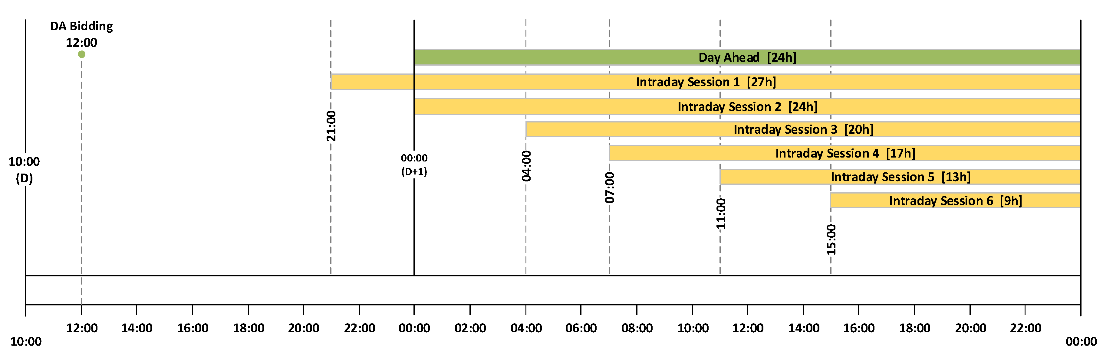
Figure 1 depicts the time horizon of both DA and ID sessions. The DA session receives bids until noon to be delivered later for the period between 00 h to 23 h of the following day. For the ID market, each of the sessions closes two hours and fifteen minutes before delivery, for the following delivery periods:
- ID1: from 21 h (day D) to 23 h (day D + 1) (27 h)
- ID2: from 00 h to 23 h (24 h)
- ID3: from 04 h to 23 h (20 h)
- ID4: from 07 h to 23 h (17 h)
- ID5: from 11 h to 23 h (13 h)
- ID6: from 15 h to 23 h (9 h)
The standardized futures contracts (e.g., quality, volume, quantity, period) traded in Portugal and Spain are responsibility of the OMIP derivatives exchange market and have daily mark-to-market [36]. OMIP major objective is to provide clients with tools to cover and manage market risks, such as price variation and volatility [37]. The market model allows institutions with know-how in the risk management realm to take on this important role for its own account or on behalf of third parties. The activity and prices generated on OMIP are extremely useful indicators of the economic activity regarding electrical energy, which was the main reason to include the information about the settlement price of the daily future contracts in the spot price forecasting model.
2.2. Data Description
Despite the availability of historical price data since mid 2008, the majority of the system (or exogenous) variables (see Section 2.2.2) have a smaller historical period available. Therefore, the period considered for the fitting and evaluation of the proposed forecasting models was confined to two years, from June 2015 to June 2017.
2.2.1. Day-Ahead and Intraday Price Data
Market data, for both DA and ID sessions, was collected from the public repositories of both Iberian transmission system operators, REN [38] and REE [39]. For the aforementioned period, the dataset characteristics are summarized in Table 1. Although the price forecasts studied on this work were produced for the Portuguese side, there were only 6.6% hours with market splitting between both Iberian countries, with an overall difference of just 0.29 €/MWh.
Regarding the number of records, the ID1 has the highest number since it comprises 27 h. As we progress through the delivery day, the length of each ID session decreases from 24 h to 9 h and so it does the number of records. Looking at the average price for each session, it is possible to observe an increase from the first to the last ID session, with the exception of ID2. As for the standard deviation, its values are almost constant throughout the DA and ID sessions. When evaluating the min/max values, the zero price was reached in all sessions, while the maximum value allowed in the MIBEL (i.e., 180.3 €/MWh) was reached in ID1, 2, 3 and 6.
Figure 2 depicts the hourly price time series of the DA market, considering the period under study. The blue shaded area emphasizes the period between 1 January 2017 and 10 February 2017, which exhibited the highest prices during this two years period. When applying statistical learning methods heavily dependent on the availability of sufficient historical data with high (or low) price regimes, it is expected that periods like this one will pose a challenge due to the non-existence of historical similarity.
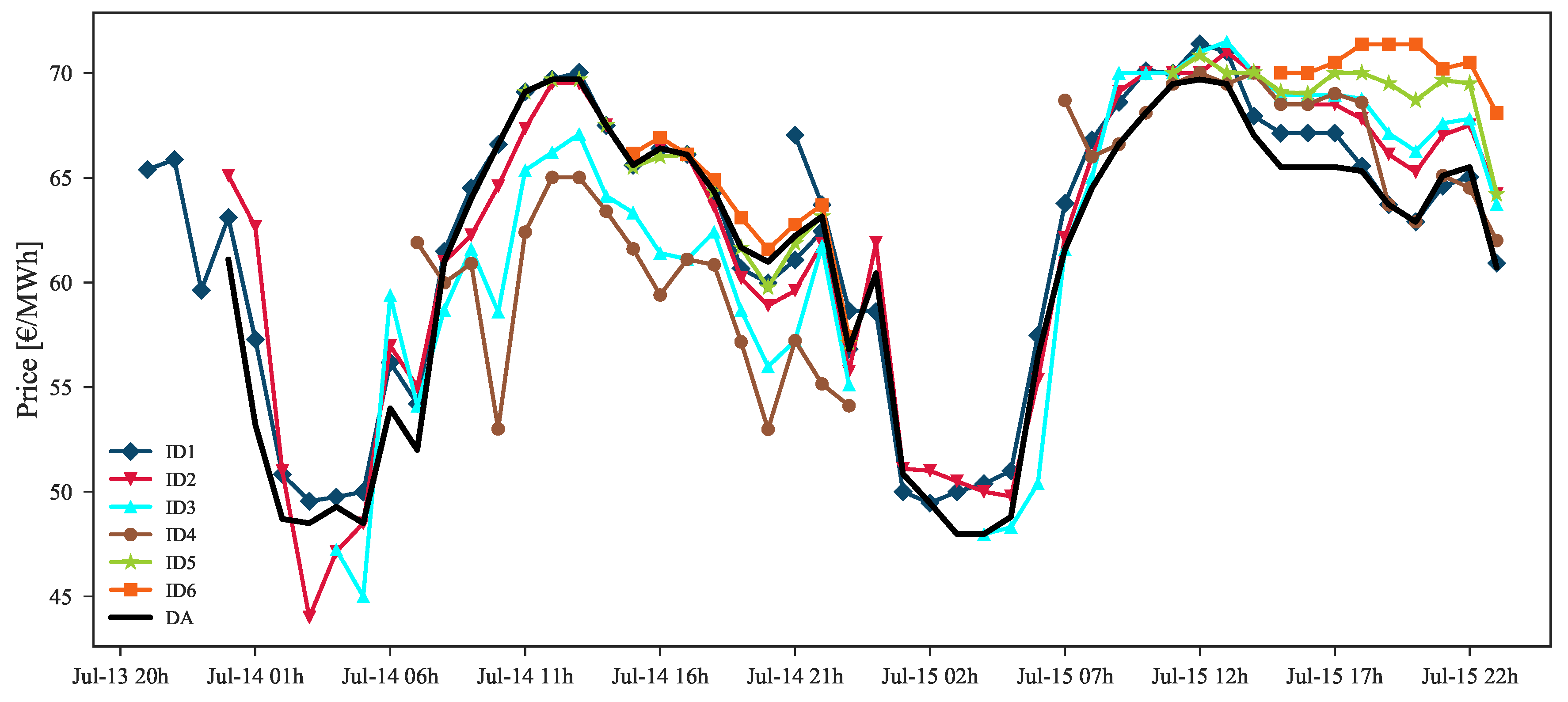
Analyzing Figure 3, which depicts an example of DA and ID hourly prices, it is noticeable that all the ID sessions are strongly influenced by the DA prices. This is expected as the ID is an adjustments market. Moreover, each ID session is highly correlated with the previous one. This observation was also confirmed by the data analysis presented in [33] for the MIBEL price data.
2.2.2. Iberian System Data
The system (or exogenous) variables considered for the forecasting model are listed in Table 2. Historical data was gathered from the ENTSO-E Transparency platform [40], which covers the large-scale generation technologies, system load, hydro reservoirs capacity and the NTC values between Portugal and Spain. Forecasts for the total renewable energy generation and load were extracted from the REN e REE market platforms. Furthermore, information from the settlement price of the daily contracts from the Iberian derivatives market [41] was also retrieved which, as mentioned in Section 1, represents a novelty in comparison with the state of the art.
3. Price Forecast Methodology
3.1. Forecasting Framework for the Day Ahead Market
Non-stationarity and high volatility are two notorious characteristics of electricity prices time series, representing major challenges to price forecast accuracy in any forecast horizon. Although some of these particular characteristics can be successfully modeled by statistical learning algorithms after a careful feature selection, extreme scenarios such as price spikes or very low or high price regimes are still specially difficult to forecast, particularly when constrained by a reduced set of historical data (i.e., less than two years).
By exploring statistical algorithms capable of generating probabilistic forecasts, it is possible to have a probabilistic representation of future uncertainty associated to each lead-time in the forecast time horizon. The definition of an “optimal” set of explanatory variables combined with the correct parameterization of statistical learning algorithms are two essential steps that must be considered by the forecaster to produce sharper probabilistic forecasts (i.e., reduced uncertainty) while guaranteeing that the forecasted set of quantiles is well calibrated, that is, low deviation between empirical and nominal quantile proportions (see Section 4.2 for mode details about forecasting skill properties).
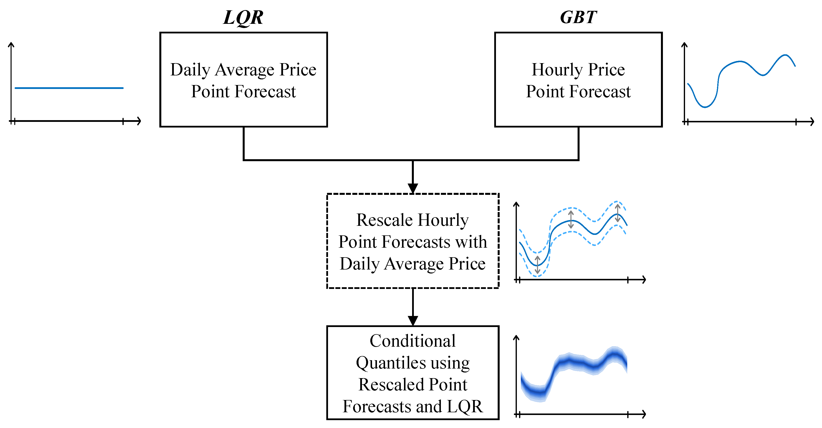
This section describes an extensive and descriptive feature selection analysis and a forecasting framework that conciliates two different statistical learning algorithms—Linear Quantile Regression (LQR) and Gradient Boosting Trees (GBT)—capable of generating point and probabilistic forecasts (i.e., set of quantiles between 5% and 95% with a 5% increment) and two distinct temporal resolutions, i.e., daily average and hourly prices. As depicted in Figure 4, the framework has the following steps:
- Daily average price point forecast, using LQR;
- Hourly price point forecast, using GBT;
- Rescale of the hourly forecast using the daily average price forecast;
- Forecast the conditional quantiles by applying the LQR to the rescaled hourly point forecasts.
3.1.1. Daily Average Price Forecast
The daily average price forecast for day is obtained by applying LQR to minimize the mean absolute error [42]. Let Y be a random variable and X a set of explanatory variables. The quantile regression model for the -quantile may be written as:
Where denotes the cumulative distribution function of the errors and where the functions are distinct for each quantile. This implies that the conditional -quantile of order of Y knowing X can be defined as:
In LQR, is a linear function of x. It assumes that are i.i.d such that , where is a vector of unknown parameters.
The conditional -quantile is computed using a pinball loss function, defined as:
Generally, the conditional quantile is the solution of the minimization problem:
For the point forecast of the daily average price, the conditional median (i.e., ), which corresponds to minimize the expected absolute loss—), is used as loss function. The implementation from the Python open-source Statsmodels library [43] was used in this work.
Besides the statistical algorithm, finding the best set of explanatory variables is a key factor to obtain high quality forecasts. A preliminary analysis (procedure described in Section 4) over the available data determined that day-ahead average price forecasts are mainly dependent on the settlement price of daily futures contracts (FPOMIP) and the average of hourly wind power forecasts (FW). Other variables such as PV (SPV) or coal-based generation (C) also may be considered as they increase the robustness of the forecasting model.
Table 3 presents the numerical results of the classical point forecast error metrics (mean absolute error—MAE, root mean square error—RMSE and mean absolute percentage error—MAPE) obtained with the best set of explanatory variables for day-ahead daily average price forecast.
This batch of explanatory variables was defined with the process described in the following paragraphs, which main goal was to remove redundant information and maintain only the most informative variables.
Starting with a base model (), exclusively composed by calendar variables (CWd, CM) and lagged daily average wholesale prices (, ), the two major forecasting skill improvements are obtained when daily price of futures contracts and daily average of forecasted wind power are added to the base model, resulting in models and respectively. Specifically, considering the MAE, RMSE and MAPE metrics, improvements of 40.77%, 39.52% and 35.88% were obtained with the inclusion of futures contract price information. Additionally, the inclusion of the forecasted wind power increases the improvement on the three aforementioned scores to 46.40%, 45.69% and 42.54% respectively, when comparing to the base model.
The remaining variables slightly contribute to improve the overall performance of the forecasting model, with improvements in the order of 1% for each score. Nonetheless, the addition of these variables improves the overall robustness of the forecasting model when combined with the remaining variables due to cross-effects uncovered by the machine learning algorithm.
The final model () significantly outperforms the base model (), with improvements of 47.81%, 47.68% and 44.73% on MAE, RMSE and MAPE scores.
3.1.2. Hourly Price Point Forecast
The increasing integration of renewable energy in electricity markets is originating non-linear relations between price and exogenous variables like wind power penetration [17]. Therefore, GBT was used in this work to produce point forecasts for the hourly prices.
GBT is a machine learning algorithm that can be applied to both classification and regression problems. It produces a statistical model that is an ensemble of weak learners [44]. In this work each learner is a regression tree. The numerical optimization is solved by a steepest-descent minimization procedure in function space. The ensemble of regression trees is trained sequentially by estimating a new tree according to the output of the previous iterations. More specifically the GBT algorithm can be described as follows: Given the inputs: training set , a loss function , M number of estimators to fit and as set of parameters for the regression tree.
- Initialize model with a constant value, which can be the average of the target value .
- For :
- (a)
- Compute the negative gradients:
- (b)
- Fit a regression tree to the negative gradients , i.e., train it using the training set .
- (c)
- Update the model as follows:
- Output
The major challenge in the application of GBT algorithm is to fine tune the different types of hyperparameters, namely:
- (i)
- tree-specific parameters, affect each individual tree in the model.
- (ii)
- boosting parameters, affect the boosting operations in the model.
In this work, the GBT hyperparameters were estimated using the Bayesian optimization algorithm [45]. The Bayesian optimization and GBT implementations can be found in the Python open-source bayesian-optimization and scikit-learn [46] libraries, respectively.
Achieving high quality results on forecasting problems by exclusively relying on a selection of the statistical algorithm to be applied is often not enough. Hence, an important task that the forecaster must consider involves using domain knowledge on the available data in order to identify important raw variables and generate new variables (see [47] for a detailed example), capable to reinforce seasonal patterns or even uncover new dynamics previously hidden in the raw dataset. A detailed analysis of the feature selection process is presented in Section 4. The final model, the one with best performance, is composed by the following variables:
- Calendar variables. Hour, day of the week and month variables are used to capture the seasonal component of the price time series.
- Lagged price information (lags, ) with respect to a specific lead-time t + k, where t represents the last hour of market session for day D and k a specific hour in the forecast horizon of day D+1. It is well-known in the literature that day-ahead prices () demonstrate a significant correlation with the price curves of the previous day () and the same day in the previous week () [8].
- Wind power penetration. Like in Denmark [31], wind power generation occupies a large share of the energy mix of Iberian peninsula and has a significant direct impact on the definition of market clearing prices. The inclusion of this variable contributed to improve overall point forecasting accuracy and reduce the forecast uncertainty.
- Coal-based generation. Periods in which the system baseload is mainly supplied by coal-based power plants will be normally characterized by higher electricity prices. This variable provides the model with additional information regarding the share of coal in the system load.
- Hydro reservoir capacity. The Iberian Peninsula is characterized by having a significant amount of hydro power plants with reservoir. Despite the low marginal costs, this technology is highly dependent on seasonal patterns of rainfall. This variable represents the current level of water stored in the reservoirs, improving the forecast model capacity to differentiate low (reservoir full) and high (reservoir empty) price regimes.
- System load forecasts. Given its dependency on electricity demand, market clearing prices usually follow its daily and weekly seasonality patterns. That is, peak load periods are usually accompanied by an increase of spot prices and vice versa. Accommodating this information improves the model’s capacity to generate sharper probabilistic forecasts. The ability to model weekly seasonality patterns such as weekend lower prices or holidays is also enhanced.
- Solar PV and thermal power forecasts. As other RES, solar technology has low marginal cost and will almost always be dispatched by the market clearing mechanism. Considering that a small share of the energy mix is occupied by this generation type, the impact of this information in the forecasting model remains residual. However, the inclusion of these variables helps to model days when peak periods of PV and thermal generation, on top of the remaining generation sources, lead to a decrease of the day-ahead spot price.
- Settlement price of daily futures contracts. This information, obtained from the OMIP derivatives market, when included in hourly day-ahead spot price forecast model, represents a reference to the average value of hourly price forecasts. While its inclusion substantially improved the quality of point and probabilistic forecasts by resolving some of the under and over estimation situations, it is demonstrated in Section 4 that extreme low and high price levels, only with a small subset of representative historical data, are still very difficult to forecast. For these cases, a rescaling solution is proposed in Section 3.1.3.
The datasets used to train the predictive model’s comprise all in the information available prior to the launch time of the forecasting models. A detailed description of the temporal framework of each daily forecast run is available in Section 4.1.
3.1.3. Point and Probabilistic Forecast Rescaling
This approach aspires to solve some of the non-stationarity related problems verified in hourly forecasts where a significant decrease of forecast accuracy was observed in extreme low and high price regimes, in particular a high forecast bias that motivated the rescaling of the point and probabilistic forecasts. To address this problem, the proposed framework is capable to properly readjust the hourly price forecasts, generated with the GBT algorithm, using information about the daily average price forecast generated with the LQR algorithm.
Assuming a specific lead-time of interest (k = 1, …, 24) in the DA market session of day , and as the daily average price forecast and hourly price point forecasts (quantile 50% that minimizes mean absolute error) correspondingly, the rescaling phase is decomposed in the following steps:
- Calculate the daily average from the hourly price forecasts :
- Determine the scale coefficient that is applied to so that it matches the value of :
- Rescale by applying the coefficient :
- Apply LQR using as inputs the rescaled hourly predictions , wind power penetration and system load forecasts for day , as well as calendar variables. Each -quantile is modeled as follows:where are unknown coefficients dependent on to be determined from the observations of the set of explanatory variables. The calendar variables CH, CWd and CM are decomposed into cosine and sine parts, C*, cos and C*, sin. For example, and with . For variables CWd and CM we have and respectively.
The rescaled forecasts have a lower forecast error compared to the GBT output, which improves the sharpness and calibration properties of forecast intervals (as showed in Section 4), and comprises information from the set of explanatory variables. Therefore, and also because the error bias was already reduced by employing a variance minimization method that uses weaker learners with high variance and low bias (i.e., decision trees [48]), a parsimonious and linear model is applied in this last level to have a “stable” forecast of the conditional quantiles.
3.2. Forecasting Framework for the Intraday Markets
For intraday markets, the previous sessions clearing prices are available at the moment of each forecast run. Considering the relation between all the sessions depicted in Figure 3, the price of futures contracts is no longer relevant for the forecasting model of intraday markets. Also, the methodology used to rescale the day-ahead market price forecasts is not used for these market sessions, as the strong reference of past price sessions by itself is enough to obtain properly scaled forecasts.
After an extensive feature test process it was found that, for these adjustment markets, simple models yield the best results. These findings are supported by [33], where higher forecast quality was obtained by exclusively relying on the hourly prices of previous intraday and day-ahead sessions as model inputs. The present work shows that the same assumption is valid for probabilistic forecasts.
In this work, by applying a LQR with hourly prices of previous sessions and calendar variables as model inputs, high quality results were achieved in both point and probabilistic forecasts. Analogously to the day-ahead market, the fitting of forecasting model’s is performed every day for each intraday session and the forecasts are computed for the respective market programming periods illustrated in Figure 1.
Let be the linear model for the ith intraday session (), the observed prices for day ahead market and representative of the prices for j intraday sessions , the LQR used to forecast the market prices of intraday session i is defined as:
where c comprises the calendar input variables in the model:
Note that, in Equation (11) the model for intraday session i includes observed prices from all previous sessions.
4. Results and Discussion
4.1. Simulation of the Operational Forecast Scenario
Short-term price forecasts are only relevant if generated prior to the session gate closure. Considering the timeline presented in Section 2.1 for the DA and ID sessions, it is important to underline that the methodology presented in this paper replicates an operational forecast scenario where the data extraction and forecasts computation stages are conditioned to the information publicly available prior to market closure, guaranteeing that forecasted prices can be used by market agents in their decision-making processes.
Figure 5 depicts the temporal framework of each forecast run. Assuming t as market sessions gate closure (see Figure 1), each forecast run is organized in three distinct phases: (i) retrieve system and market data; (ii) statistical model’s fitting; (iii) deliver forecasts.
Accordingly, all the necessary data to be used by the forecasting models is retrieved 60 min prior to gate closure ( min). Then, a model’s fitting is executed. Finally the forecasts are delivered 30 min before market gate closure ( min).
This sequence of events is repeated every day for each market session, guaranteeing that the most recent data is incorporated into the dataset used to fit the forecasting models. In each day, the training dataset used to fit the forecasting models comprises all the Iberian system data from 12 June 2015 until the forecasts launch time.
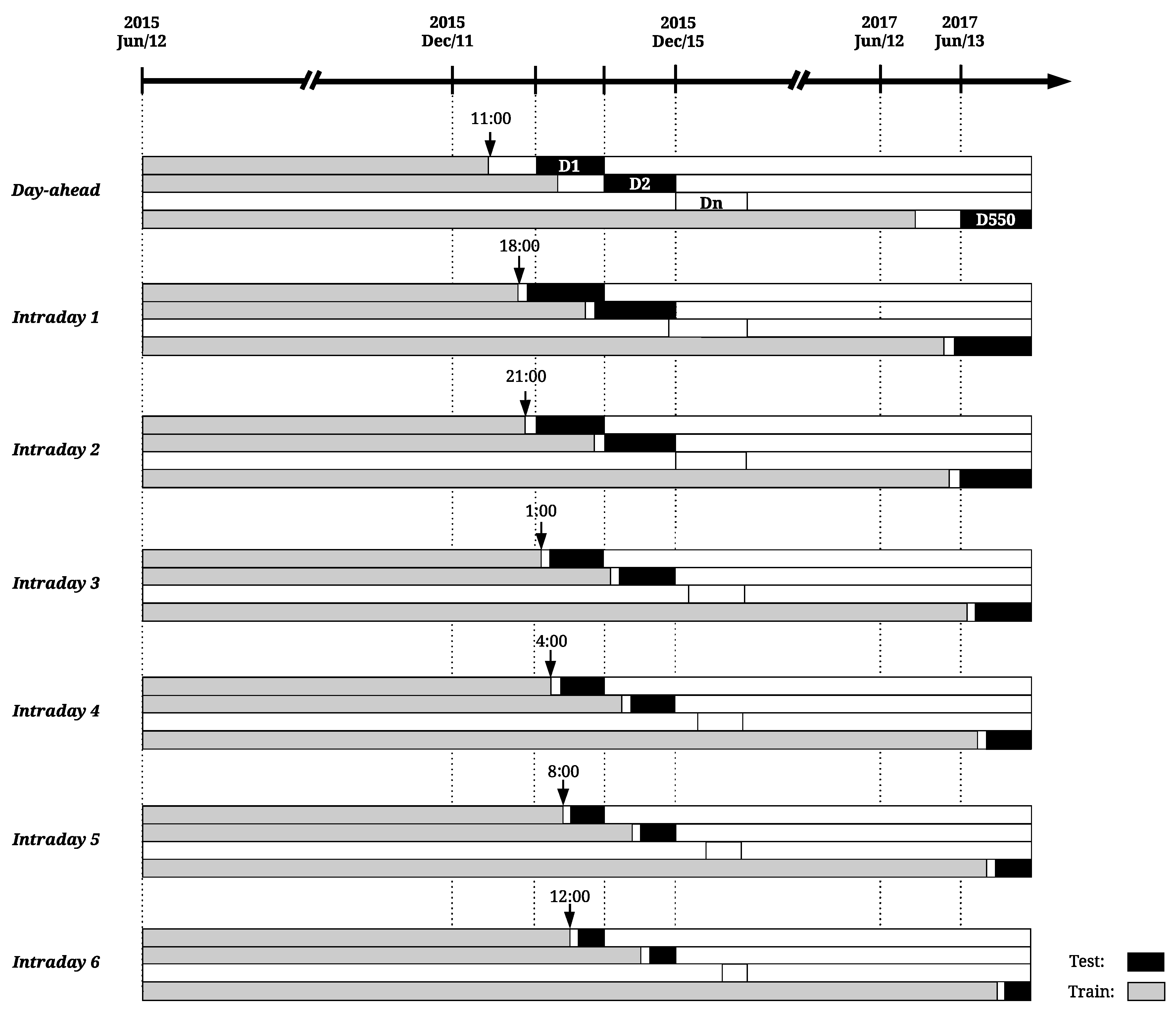
Considering the aforementioned temporal framework, a rolling window approach is here used to test each model performance along the available historical data. This test methodology is illustrated in Figure 6, where gray colored bars represent the training data gathered from 12 June 2015 until 50 min before session gate closure (see Figure 5) and black bars the test data of each rolling window iteration or, in other words, each day-ahead or intraday session programming period.
In the first iteration of the rolling window process, the models are fitted with six months of data (June–December 2015) and the forecasts are generated for 12 December 2015 (day D1 of Figure 6). This process is repeated until 13 June 2017 (day D550 of Figure 6), making a total of 550 iterations (or number of days in the test sample).
For DA and ID2 market sessions, the forecasts are computed at the present day (D) for the intervals 1 to 24 of day ahead (). It is important to stress that the start of the datasets used for fitting is maintained through all the validation process, forecasting models are trained in a daily basis and the size of train dataset increases in each iteration, accommodating recent system and market data.
4.2. Forecasting Skill Scores
The accuracy of point forecasts (i.e., quantile 50% in this work) was evaluated by the root mean square error (RMSE), the mean absolute error (MAE), and the mean absolute percentage error (MAPE). On the later, all the absolute percentage values above 100% were removed to exclude a small subset of cases with abnormally high percentage error due to price values close to zero, which introduced extreme and unrealistic penalties in the MAPE calculation.
The quality of probabilistic forecasts was evaluated with the following metrics: calibration, sharpness and continuous ranked probability score (CRPS).
Empirical probabilities (or long-run quantile proportions) should asymptotically approach the nominal (or subjective) probabilities. The calibration metric is used to assess this important property [49]. This difference between empirical and nominal probabilities can be denominated as bias of the probabilistic forecasts and is usually calculated for each quantile nominal proportion , as follows:
for a given horizon , where is the indicator function evaluating if the actual price lies below the quantile forecast , over the evaluation set .
Sharpness quantifies the uncertainty of the probabilistic forecasts [49], which numerically corresponds to compute the average interval size between two symmetric quantiles (e.g., and with ) as follows:
with nominal coverage rate and horizon .
Sharpness and calibration are intuitive properties, but can only be exploited in a diagnostic mode. On the other hand, CRPS is an unique skill score that provides the entire amount of information about a given method’s performance and encompasses information about calibration and sharpness of probabilistic forecasts. The CRPS metric was adapted to evaluate quantile forecasts (for more details see [50]) as follows:
where is quantile loss function defined in Equation (3), the actual observed price at horizon and the quantile price forecast. The CRPS is given as a percentage of the maximum price 180.3 €/MWh.
Each of these metrics were calculated considering all the forecasts generated between 12 December 2015 and 13 June 2017.
4.3. Numerical Results: Day-Ahead Market
When working with datasets composed by a large number of explanatory variables, it is appropriate to apply domain knowledge combined with proper feature selection methodologies to remove unnecessary or redundant information that might decrease the performance of forecasting models.
Different feature exploration techniques can be used to narrow a large number of variables into a smaller subset that retains the most representative information. The feature evaluation methodology described in this work comprises three distinct phases. Firstly, the individual importance of every system variable to the forecasting skill is examined. Secondly, the cross-effects between variables are examined. Finally, a subset of explanatory variables capable of producing high quality hourly price forecasts is presented and the importance of the rescaling framework, described in Section 3.1, is evaluated.
Given the extent of information available in this work, each variable is referred in the following subsections accordingly to the nomenclature presented in Table 2.
4.3.1. Analysis of Individual Variables Effect
A preliminary analysis conducted with the full set of explanatory variables concluded that calendar variables and lagged wholesale electricity price need to be included in all models since it substantially improved the point and probabilistic forecasting skill. Therefore, a base model exclusively composed by these variables (B = {CH, CWd, CM, P}) was defined to compare and assess the importance of the remaining variables.
Table 4 summarizes the impact of each variable on point and probabilistic forecasts. The models are presented in descending order according to the MAE improvements on the aforementioned base model (B). The improvement over the base model is presented inside brackets.
By examining Table 4, four significant improvements on point and probabilistic forecasts are observed regarding the inclusion of daily price of futures contract (FPOMIP), wind power penetration (FWPen), wind power generation (FW) and residual system load (FLRes) forecasts. Each of these variables contains information that improves a base model exclusively constituted by calendar data and past (or lagged) prices.
Comparing the improvement related to the inclusion of wind power generation and penetration, it is verifiable that the latter contributes significantly more to point and probabilistic forecast quality, providing an additional improvement of 1.22%, 2.14%, 0.43% and 1.08% on MAE, RMSE, MAPE and CRPS respectively. The remaining variables, when included separately in the base model, showed either residual or negative improvement in each score.
It is important to underline that this analysis only considers the relation effects between calendar variables, lagged prices and each new variable. Such evaluation provides significant knowledge about the importance of each variable when added alone to the forecast model and enables the creation of simple models with a small subset of information.
4.3.2. Analysis of Variables Cross-Effects
After the identification of the variables with high individual impact on the forecasting skill, it is important to assess if these have complementary or redundant information when included simultaneously in the forecasting model. In some cases, due to cross-effects between variables learned by the statistical model, some variables that led to low improvement, when individually included in the base model (see Section 4.3.1), can improve the price forecast skill in specific events if combined with other variables in the model.
In this subsection, the cross-effects impact of the variables set is evaluated. For this purpose, a forward selection process is presented. It involves the definition of a base model to which new variables are progressively added, according to its individual importance to the forecasting skill (defined in Section 4.3.1 Table 4). In each iteration of this process, the importance of every combination of inputs to the forecast skill is evaluated by computing the relative improvement over the base model.
Table 5 presents every combination of variables tested in this selection process. Analogously to the previous section, Mbase represents the base model, composed by calendar variables and lagged prices. Gray colored cells mark the new feature included in each iteration.
In a final stage, the redundant information contained in model M21 is removed by an exploration process that tests different combinations between the 22 explanatory variables. Considering that 22 system variables are available (calendar variables remained constant thorough all tests), a total of 4,194,303 () possible combinations should be considered. However, performing such number of combinations would result in an extensive and unfeasible evaluation process. Instead, an analysis of distinct combinations of variables combined with a sensibility analysis of each variable importance resulted in a reliable subset of variables that maximized the performance of point and probabilistic models, represented by Mfinal.
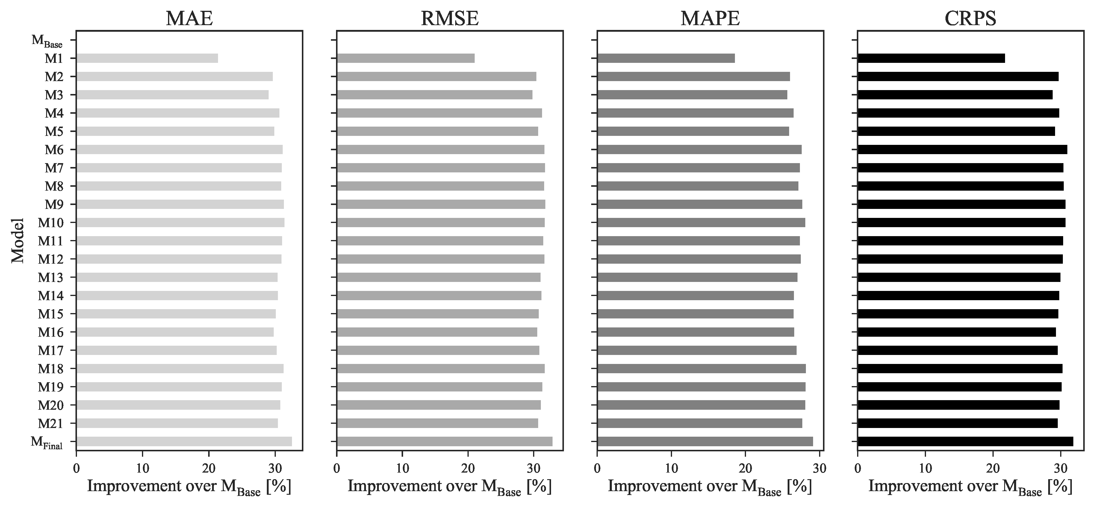
A comparison between models M1 and M2 of Figure 7 reveals that, by adding wind power penetration forecasts on top of future energy contracts settlements prices, it is possible to obtain an 10.54%, 11.93%, 9.13% and 10.12% improvement on MAE, RMSE, MAPE and CRPS scores, respectively. These two variables, besides demonstrating high importance to the forecasting skill when individually included in the forecast model, also have complementary information and increase the precision and robustness of the model while decreasing its uncertainty and point forecast errors.
For the remaining variables, the improvements are significantly less noticeable. Variables such as wind power and residual load forecasts, which led to high improvements when individually included in the base model (see Section 4.3.1), showed some redundancy when included in a more complex model composed by the variables FPOMIP and FWPen.
In contrast, by observing the higher improvements of models M6, M9, M10 and M18 on every metric, it is possible to verify that variables such as solar thermal and PV power, hydro power generation and hydro reservoir capacity, when combined with a predefined subset of other explanatory variables, contribute to increase the forecasting skill. It is important to underline that these variables showed a negative impact on the forecasting skill when added separately to the base model (see Table 4). However, due to cross effects between all model’s variables, the introduction of these variables improved the overall accuracy.
With that being said, model Mfinal presents the best subset of explanatory variables for day-ahead market forecast. By cleaning the redundant information it was possible to reduce the number of explanatory variables from 25 to 11 while keeping the most insightful information and maximizing the predictive performance of the forecasting model. Variables such as residual load or wind power generation that demonstrated a great improvement on forecast quality when individually added to a base model, were discarded in detriment of system load and wind power penetration forecasts as they complemented significantly better the information provided by the remaining inputs. The improvements of a model trained with this final batch of explanatory variables over the base model were 32.54%, 32.87%, 29.08% and 31.85% on MAE, RMSE, MAPE and CRPS scores.
After finding the best set of explanatory variables, it was only possible to enhance the forecasting skill by rescaling the forecasts with the methodology described in Section 3.1.3.
4.3.3. Benefits from Rescaling Day-Ahead Price Forecasts
This subsection presents a detailed comparison between the hourly forecasts obtained using the model analyzed in the previous Section (Mfinal) and the forecasts obtained after forcing the daily average to be equal to the forecasted daily average price (see Section 3.1.3). Table 6 shows the results of this comparison in terms of MAE, RMSE, MAPE and CRPS.
Just by applying the rescaling procedure to the obtained hourly forecasts (Mrescaled) and comparing with Mfinal, an improvement of more than 10% was achieved when looking to both MAE and RMSE metrics. Furthermore, it also significantly improved the MAPE (4%) and CRPS (8.8%).
When applying the LQR to the rescaled point forecasts to produce quantiles forecasts, two explanatory variables were tested: system load forecasts (FL) and wind power penetration forecasts (FWPen). By adding these two variables it was possible to decrease the MAE/RMSE by 0.13%/0.17% and 0.98%/1.17% respectively. Moreover, a positive impact in uncertainty forecast was also verified since an improvement of more than 4% was obtained in CRPS.
With the best model (Mrescaled, {FL, FWPen}), the MAE was fixed in 3.03 €/MWh, the RMSE in 4.04 €/MWh, the MAPE in 8.54% and the CRPS in 1.22%.
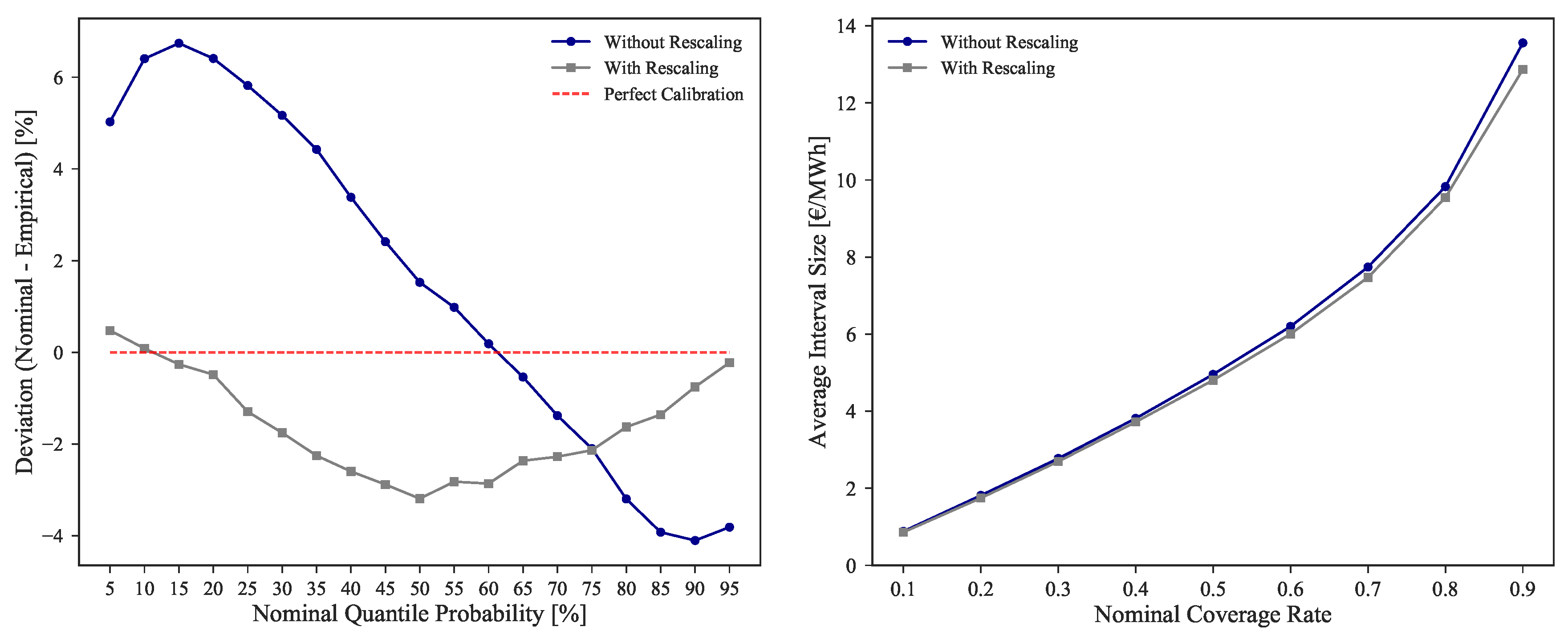
Additionally to the CRPS improvement, the calibration and sharpness were also improved. Figure 8 shows the comparison between Mfinal and Mrescaled, {FL, FWPen} for these two metrics. While a minor improvement is noted on the sharpness of forecasts, in the case of calibration it is possible to observe an absolute improvement of 53.26%, more notorious in the lower and higher quantiles.
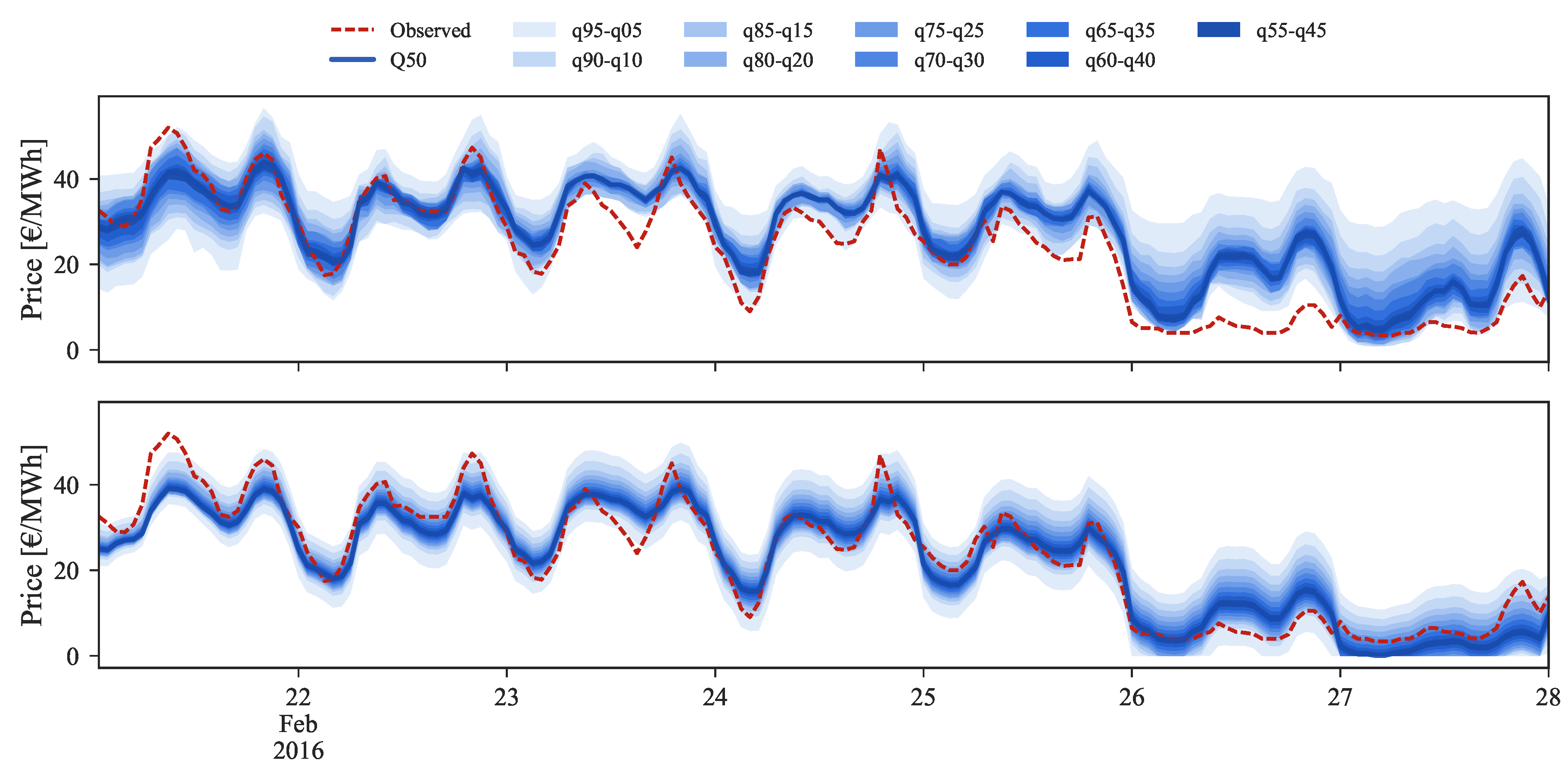
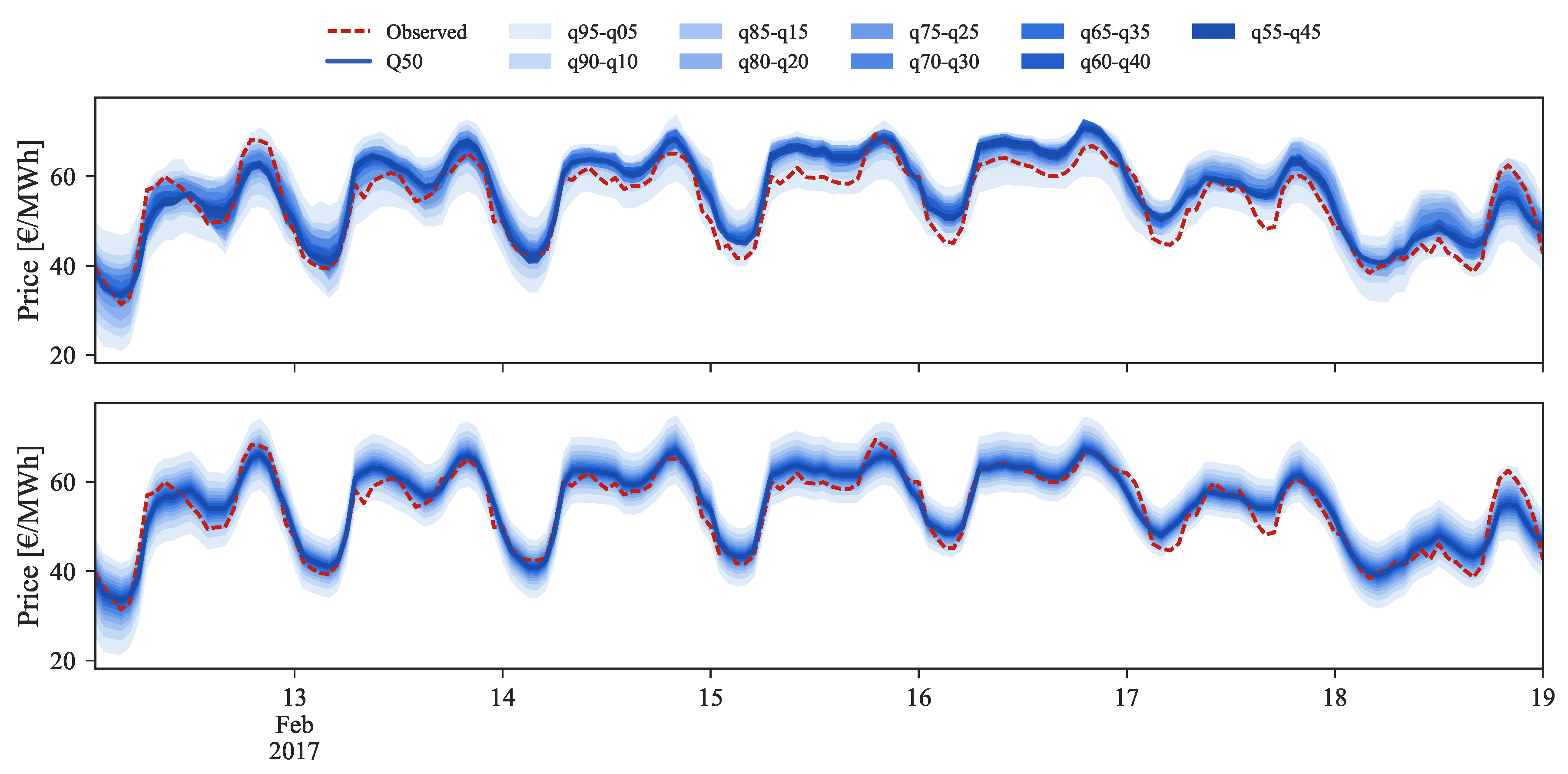
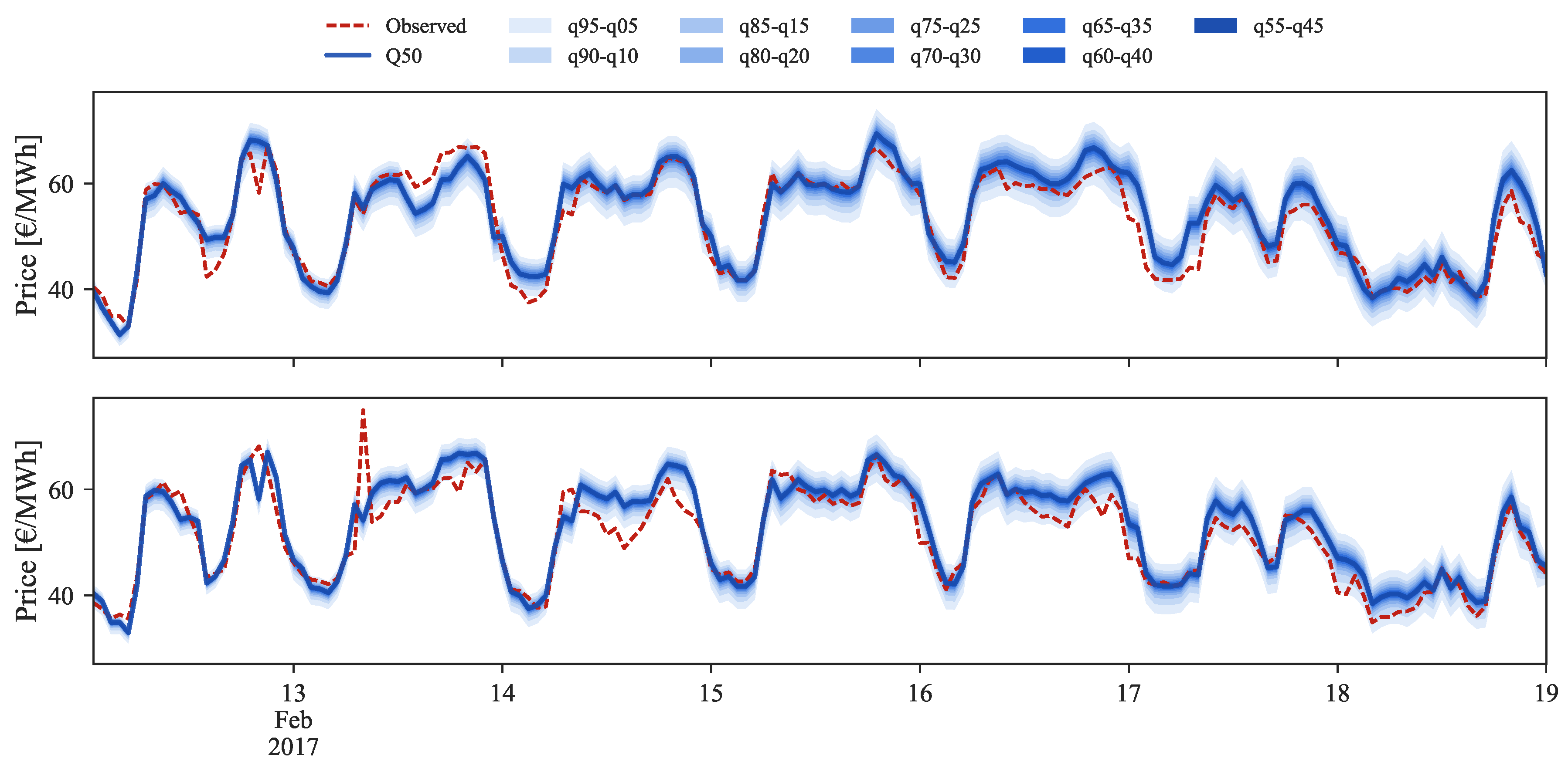
Figure 9, Figure 10 and Figure 11 depict a visual comparison between the forecasts before (top) and after (bottom) the application of the rescaling process. Each set of figures illustrates three distinct price regimes: low, medium and high prices.
Starting by the low prices regime, illustrated by Figure 9 for the period between 22 and 28 February 2016, it is easily observable on the bottom side the improvement provided by the rescaling process.
In the last two days, where the observed market price reached values close to zero, the original forecasts were unable to capture the observed price curve. By applying the rescaling, the 50% quantile is now closer to the observed values and the uncertainty band (or set of forecast intervals) encompasses the observed price curve. Moreover, the sharpness of probabilistic forecasts was also drastically increased.
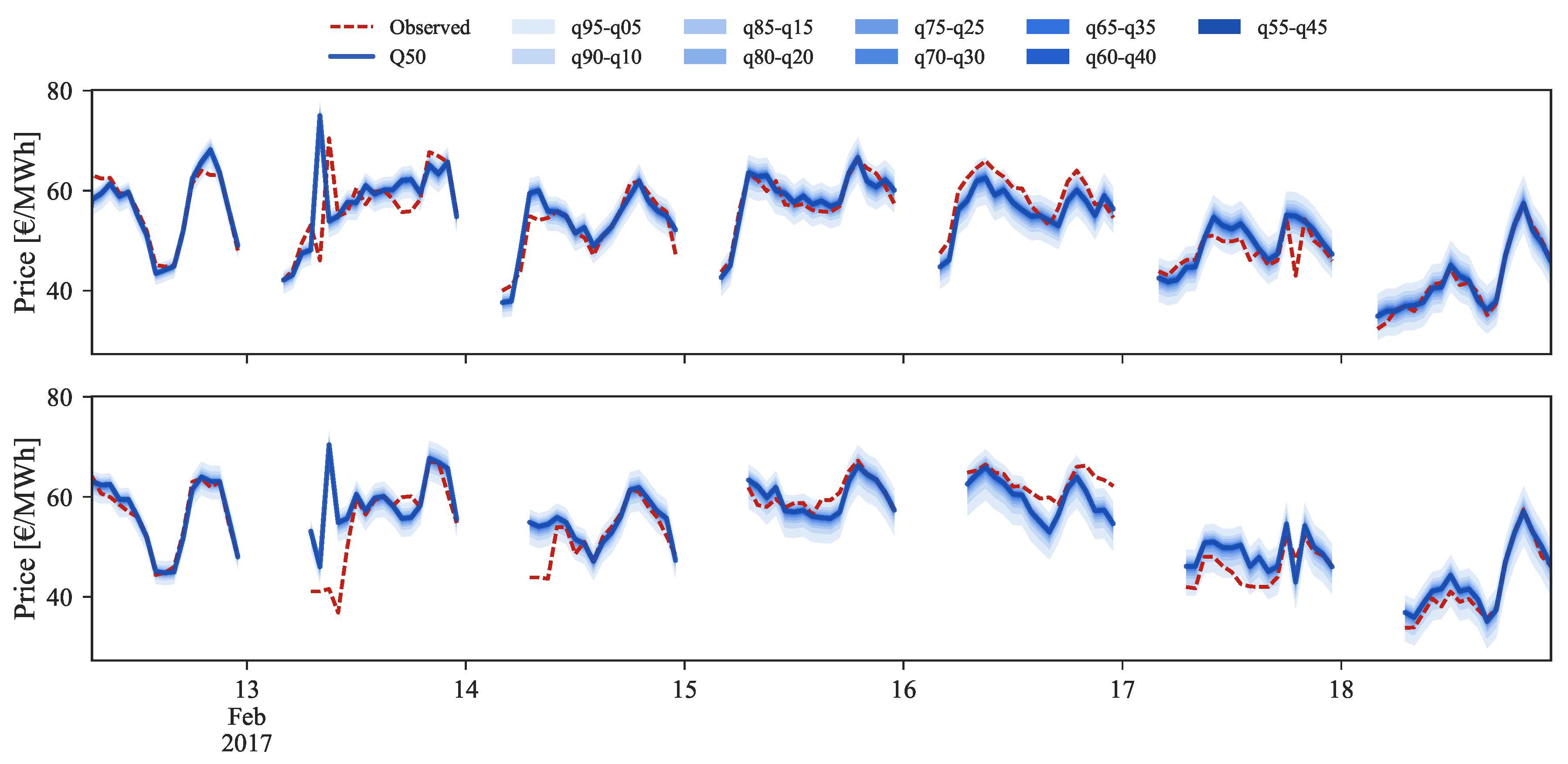
In the medium price regime (Figure 10) for the period between 13 and 19 February 2017, the quantiles distribution is well modeled and periods in which the observed price falls outside the 5% and 95% quantiles are not verified. However, the conditional median (i.e., ) often shows a bias with respect to the observed value. After rescaling, this bias disappears and an improvement in the probabilistic forecast sharpness is also observed.
Figure 11 depicts the forecasts for the high price regime for the period between 16 and 22 January 2017.
The original forecast completely misses during this period. This can be explained by analyzing Figure 2 where it is possible to observe that this price range cannot be found in the historical dataset, which impacts the performance of statistical learning methods like GBT. With the information from daily average price forecasts it is possible to capture the trend of observed prices and then rescale the original forecasts for these periods, even without any past reference in the historical dataset.
The improvements provided by the rescaling method throughout the complete range of prices are depicted in the boxplots of Figure 12. These boxplots show the MAE distribution divided by ten equally distributed price classes, as well as the percentage of forecasts with under and overestimation. The top plot corresponds to the original forecasts, while the bottom plots concerns the rescaled forecasts.
The original forecasts have a tendency to overestimate in low price regimes and underestimate in high price regimes. This bias is mitigated by the rescaling process as demonstrated in the bottom boxplot. As previously mentioned, the improvement obtained by rescaling the forecasts is lower for medium price levels. However, it is substantially high for low/high price levels as showed by the MAE reduction between the two boxplots.
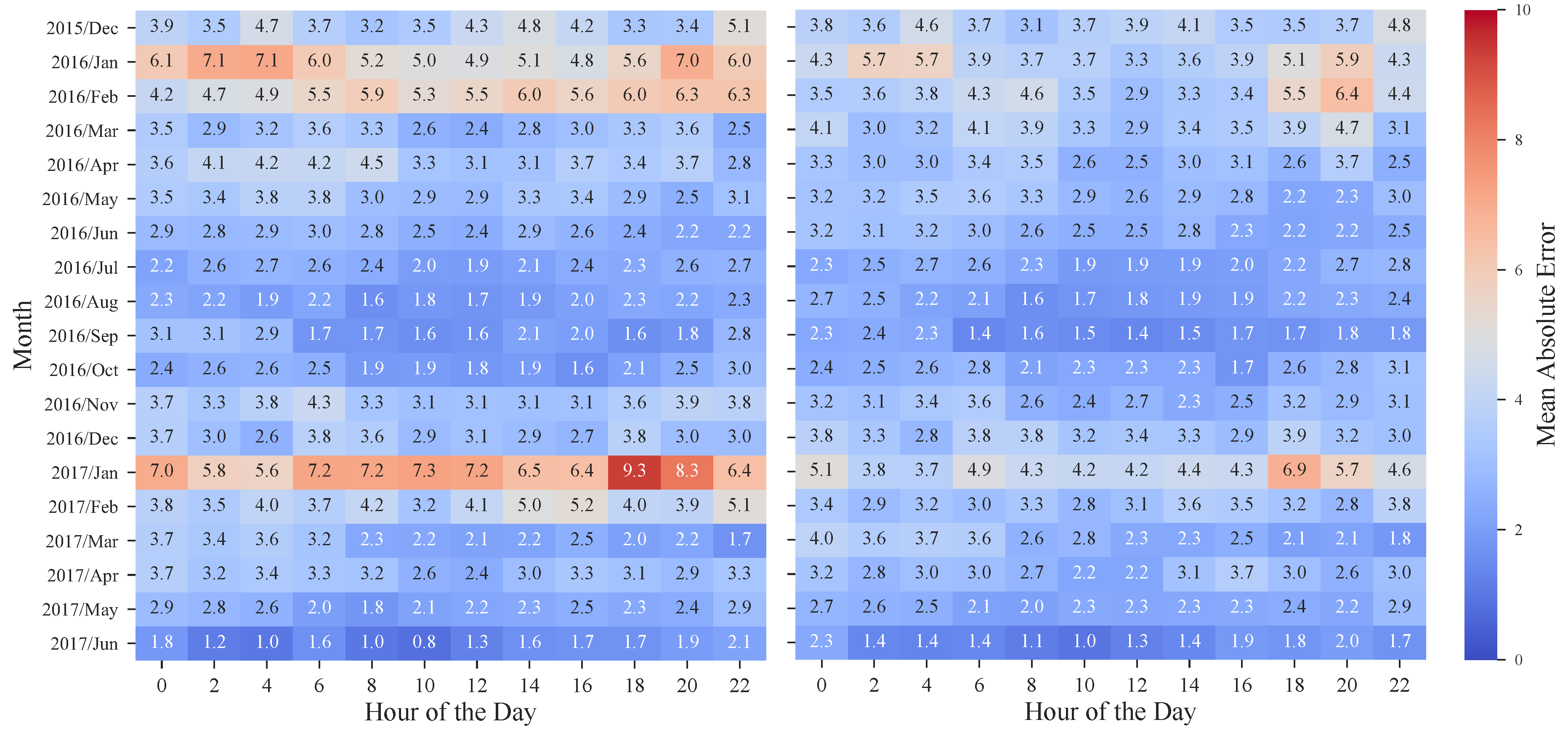
The benefits of the rescaling procedure are also emphasized by the heatmaps depicted in Figure 13, in which the MAE values for each hour and month of the period under evaluation are presented. Once again, and by revisiting Figure 2, it is possible to observe the significant improvement obtained in weeks with high prices. In January 2017, the MAE was ranging from 5.6 to 9.3 €/MWh while after applying the rescaling theses values decreased to 3.7–6.9 €/MWh. Furthermore, these results also show that, as the historical dataset increases, the forecasting error has a tendency to decrease, with the exception of atypical price periods.
4.4. Numerical Results: Intraday Markets
As mentioned in Section 3.2, it was verified that the information about hourly prices of the daily session and previous intraday sessions is highly valuable and must be considered in the forecast model. In this subsection, four distinct type of models that synthesize different sets of variables are evaluated:
- IM1—Selection of historical and forecasted system variables (see model Mfinal of Table 5) combined with price information of the previous market session.
- IM2—Forecasted system variables (see Future [D + 1] information in Table 2) combined with prices from previous market session.
- IM3—Prices from previous market session.
- IM4—Combination of the clearing prices of every preceding session (i.e., for ID2 the prices of ID1 and DA are used as explanatory variables).
Models IM1 and IM2 were defined to assess the importance of system variables (or exogenous information) to the forecasting skill. Models IM3 and IM4 are exclusively composed by previous daily and/or intraday session prices data. Model IM4 corresponds to defined in Equation (11) where, for each session i, the previous daily and intraday market sessions prices are included. In contrast, IM3 only includes information from the previous session (). These models were defined to verify the importance of this information when included alone, independently of any exogenous variables. All models accommodate calendar variables (see Table 2) as it helped to capture some daily and weekly periodicity.
Table 7 summarizes the point and probabilistic forecasting skill scores for the intraday models IM1, IM2, IM3 and IM4.
An analysis of the table shows, for each session, that there is a high similarity between the evaluation scores, with MAE, RMSE, MAPE and CRPS presenting values with similar order of magnitude.
Comparing the results of models IM1 and IM2, it is hard to settle which information provides the most accurate price forecast. The discrepancy between models only starts being noticeable for sessions subsequent to ID3, where model IM2 starts to outperform the first in every score. However, a comparison between these two models and IM3/IM4 shows that previous market session prices are sufficient and offer better forecasts for the intraday market (i.e., close to 1% improvement of IM3 over IM2 and IM1 in ID1). This observations reveal that exogenous information is not critical to achieve a good forecast quality in this type of market.
An overview of the six intraday sessions results reveals a general decrease in the forecast accuracy from ID2 to ID6 (see the upward trend on MAE, RMSE, MAPE and CRPS errors), with exception of ID4 where the models presented better performance. An hypothesis for this increase in the error relates to the trading liquidity of these markets, that decreases as it approximates to the last session. In these low liquidity periods, higher price volatility is verified along with some cases where the prices reached its maximum value of 180.3 €/MWh.
Regarding ID1, it is important to remember that it includes the last three hours of the current day (day D). These hours are the last opportunity for adjustments in day D (e.g., the Portuguese transmission system operator names this period intraday 7) and corresponds to the time period with the lowest liquidity, which makes it specially hard to forecast. Higher errors on these hours increase the overall average forecast error of session ID1.
Compared to the day-ahead session forecasting skill (see Table 6), it is possible to verify that the forecasts for intraday sessions exhibit substantially lower errors in point and probabilistic forecasts. This difference occurs mainly due to the available price references when the forecast is generated. For intraday sessions, hourly prices from the previous sessions (intraday and day-ahead) are powerful explanatory variables and are immediately available. On the other hand, for the day-ahead market, the only reference is the settlement price of daily futures contract that does not encompass information about hourly price variations. Moreover, the explanatory power of the previous day prices is considerably lower when compared to the price from previous intraday sessions.
Figure 14, Figure 15 and Figure 16 show probabilistic hourly price forecast time series for intraday sessions of days 13 to 19 February 2017, generated with model IM3.
An analysis of the plots shows that sharp probabilistic forecasts are generated for every lead time. These high sharpness levels are verified in the forecasts generated by each of the four models, being slightly inferior for IM1 and IM2. For these models, some improvements are verified in the calibration for ID1, ID2 and ID3 sessions, resulting in lower CRPS values. These results indicate that it would be advisable to generate point forecasts with a model exclusively based in past sessions prices (IM3, IM4), complemented with probabilistic forecasts generated with a model that integrates exogenous information (IM1, IM2). However, the relation between quality and simplicity is prioritized in this work. With that rationale, models IM3 and IM4 were preferred as they are capable to produce quality forecasts with the minimum number of explanatory variables.
As mentioned before, price data from previous sessions is the core information for intraday price forecasts. Yet, it is important to note that this dependency on the past session prices might compromise the performance for periods characterized by large price changes between sessions. For instance, intraday sessions 1 to 4, on 14 February 2017, depict a situation where, for the first half of the day, distinct values in price are observed in all sessions. A comparison between ID1 and ID2 observed and forecasted prices (red dashes and blue line in Figure 14) demonstrates that the model is unable to predict the price spike verified at 8:00 of ID2. This occurs due to the model dependency on ID1 where no price spike was verified. A similar price spike occurs at the following hour in ID3, which was forecasted with an offset due to the forecasts dependency on the observed price from ID2. In contrast, for the same hours ID4 presents a significant decrease in price when compared to the preceding sessions, which was then impossible to forecast by our model.
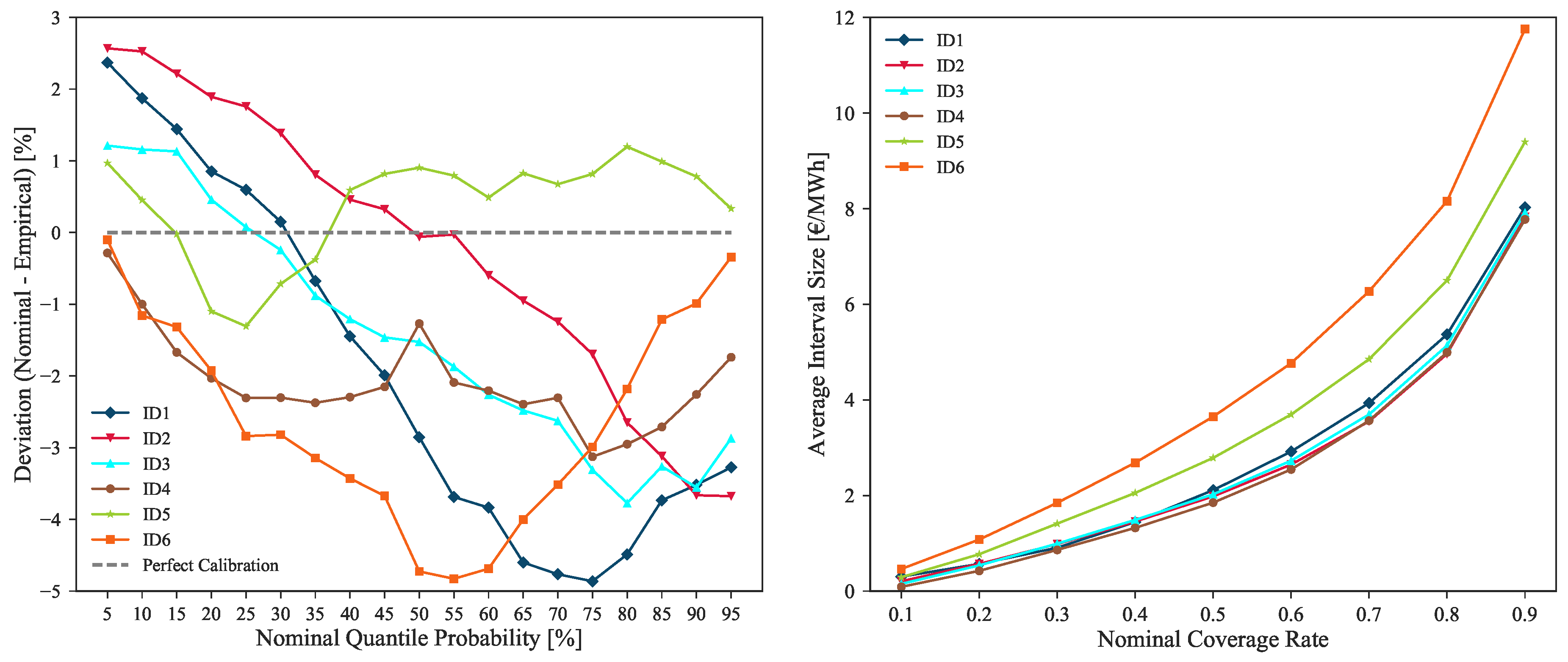
Although some of these sudden price shifts periods are impossible to model by the forecast uncertainty, the remaining lead times are forecasted with high point and probabilistic forecast accuracy. Figure 17 depicts the calibration and sharpness of the forecasts generated with model IM3 for all the intraday sessions.
The figure shows that, although sharp probabilistic forecasts are being produced for each intraday session (i.e., ID1, ID2, ID3 and ID4 close to 8 €/MWh average Q05–Q95 interval size), a good calibration is also maintained thorough every session, i.e., deviations from perfect calibration below 5% for all market sessions. These results confirm that the uncertainty of probabilistic forecasts is being correctly modeled, encompassing the observed hourly price values. As expected, in order to contain the increase in price volatility verified in sessions ID5 and ID6, lower sharpness levels can be noted for these sessions (see the higher average interval size for ID5 and ID6 depicted in Figure 17 right side plot).
5. Conclusions
This paper describes a point and probabilistic statistically-based forecasting methodology for day-ahead and intraday electricity markets. The case study was the Iberian electricity market, characterized by high integration levels of different renewable energy technologies. The proposed forecasting methodology was not driven by the choice of the statistical learning algorithm. Instead, two robust statistical algorithms from the state of the art were used: gradient boosting trees and linear quantile regression. The core contributions to improve forecasting skill were: (a) careful selection of explanatory variables with special emphasis to the information from the futures contract trading; (b) post-processing of forecasts by exploiting the forecasted daily average price. For intraday markets, this work showed that high quality probabilistic forecasts can be obtained by just exploring the prices from previous sessions.
The results showed highly accurate point and probabilistic forecasts for both day-ahead and intraday markets. In terms of point forecast, the mean absolute error was 3.03 €/MWh for day-ahead market and a maximum value of 2.53 €/MWh was obtained for intraday session 6. The probabilistic forecast results show sharp forecast intervals and deviations from perfect calibration below 7% for all market sessions.
All the data used in this work is from public repositories, which allows reproducible research and shows that accurate price forecasts can be obtained without purchasing expensive data sources (e.g., wind power forecasts, weather predictions). Although tested for the Iberian electricity market, the methodology is generic and can be replicated to other European countries. However, the final set of explanatory variables and the forecasting skill might be different, in particular for electricity markets with low integration of hydropower and/or renewable energy.
Finally, the present paper was focused in forecasting the spot electricity prices and a topic for future work is to forecast operating reserve prices which, according to [51,52], show higher variability and more frequent extreme spikes. Other topics for future work are mid-term probabilistic price forecasting and the test of alternative models, like the autoregressive logit models described in [53] or deep learning techniques with high potential to extract information from raw input variables.
Acknowledgments
The research leading to this work is being supported by (a) InteGrid project (Demonstration of INTElligent grid technologies for renewables INTEgration and INTEractive consumer participation enabling INTEroperable market solutions and INTErconnected stakeholders), which received funding from the European Union’s Horizon 2020 Framework Programme for Research and Innovation under grant agreement No. 731218; and by (b) the ERDF—European Regional Development Fund through the Operational Programme for Competitiveness and Internationalisation—COMPETE 2020 Programme, and by National Funds through the Fundação para a Ciência e a Tecnologia (FCT) within project SmartGP/0001/2015. André Garcia is acknowledged for his work in extracting all the market and forecasted data used in this work.
Author Contributions
All authors contributed to the development and test of the forecasting methods, as well as to the writing of the manuscript.
Conflicts of Interest
The authors declare no conflict of interest.
References
- Zugno, M.; Morales, J.M.; Pinson, P.; Madsen, H. A bilevel model for electricity retailers’ participation in a demand response market environment. Energy Econ. 2013, 36, 182–197. [Google Scholar] [CrossRef]
- Gholian, A.; Mohsenian-Rad, H.; Hua, Y. Optimal industrial load control in smart grid. IEEE Trans. Smart Grid 2016, 7, 2305–2316. [Google Scholar] [CrossRef]
- Morales, J.M.; Conejo, A.J.; Madsen, H.; Pinson, P.; Zugno, M. Integrating Renewables in Electricity Markets. Operational Problems, 1st ed.; International Series in Operations Research & Management Science; Springer: New York, NY, USA, 2014; Volume 205. [Google Scholar]
- Bello, A.; Bunn, D.; Reneses, J.; Muñoz, A. Parametric density recalibration of a fundamental market model to forecast electricity prices. Energies 2016, 9, 959. [Google Scholar] [CrossRef]
- Bello, A.; Reneses, J.; Muñoz, A. Medium-Term probabilistic forecasting of extremely low prices in electricity markets: Application to the Spanish case. Energies 2016, 9, 193. [Google Scholar] [CrossRef]
- Weron, R. Electricity price forecasting: A review of the state-of-the-art with a look into the future. Int. J. Forecast. 2014, 30, 1030–1081. [Google Scholar] [CrossRef]
- Szkuta, B.; Sanabria, L.; Dillon, T. Electricity price short-term forecasting using artificial neural networks. IEEE Trans. Power Syst. 1999, 14, 851–857. [Google Scholar] [CrossRef]
- Conejo, A.J.; Plazas, M.A.; Espínola, R.; Molina, A.B. Day-ahead electricity price forecasting using the wavelet transform and ARIMA models. IEEE Trans. Power Syst. 2005, 20, 1035–1042. [Google Scholar] [CrossRef]
- Shafie-khah, M.; Moghaddam, M.P.; Sheikh-El-Eslami, M. Price forecasting of day-ahead electricity markets using a hybrid forecast method. Energy Convers. Manag. 2011, 52, 2165–2169. [Google Scholar] [CrossRef]
- Nogales, F.; Conejo, A. Electricity price forecasting through transfer function models. J. Oper. Res. Soc. 2006, 57, 350–356. [Google Scholar] [CrossRef]
- Lora, A.T.; Santos, J.M.R.; Expósito, A.G.; Ramos, J.L.M.; Santos, J.C.R. Electricity market price forecasting based on weighted nearest neighbors techniques. IEEE Trans. Power Syst. 2007, 22, 1294–1301. [Google Scholar] [CrossRef]
- Kekatos, V.; Zhang, Y.; Giannakis, G.B. Electricity market forecasting via low-rank multi-kernel learning. IEEE J. Sel. Top. Signal Process. 2014, 8, 1182–1193. [Google Scholar] [CrossRef]
- Li, G.; Liu, C.C.; Mattson, C.; Lawarrée, J. Day-Ahead electricity price forecasting in a grid environment. IEEE Trans. Power Syst. 2007, 22, 266–274. [Google Scholar] [CrossRef]
- Zhao, J.H.; Dong, Z.Y.; Xu, Z.; Wong, K.P. A statistical approach for interval forecasting of the electricity price. IEEE Trans. Power Syst. 2008, 23, 267–276. [Google Scholar] [CrossRef]
- Wan, C.; Xu, Z.; Wang, Y.; Dong, Z.Y.; Wong, K.P. A hybrid approach for probabilistic forecasting of electricity price. IEEE Trans. Smart Grid 2014, 5, 463–470. [Google Scholar] [CrossRef]
- Dudek, G. Multilayer perceptron for GEFCom2014 probabilistic electricity price forecasting. Int. J. Forecast. 2016, 32, 1057–1060. [Google Scholar] [CrossRef]
- Jónsson, T.; Pinson, P.; Madsen, H. On the market impact of wind energy forecasts. Energy Econ. 2010, 32, 313–320. [Google Scholar] [CrossRef] [Green Version]
- Moreira, R.; Bessa, R.; Gama, J. Probabilistic forecasting of day-ahead electricity prices for the Iberian electricity market. In Proceedings of the 13th European Energy Market Conference (EEM 2016), Porto, Portugal, 6–9 June 2016. [Google Scholar]
- Chen, X.; Dong, Z.Y.; Meng, K.; Xu, Y.; Wong, K.P.; Ngan, H. Electricity price forecasting with extreme learning machine and bootstrapping. IEEE Trans. Power Syst. 2012, 27, 2055–2062. [Google Scholar] [CrossRef]
- Juban, R.; Ohlsson, H.; Maasoumy, M.; Poirier, L.; Kolter, J.Z. A multiple quantile regression approach to the wind, solar, and price tracks of GEFCom2014. Int. J. Forecast. 2016, 32, 1094–1102. [Google Scholar] [CrossRef]
- Nowotarski, J.; Weron, R. Computing electricity spot price prediction intervals using quantile regression and forecast averaging. Comput. Stat. 2015, 30, 791–803. [Google Scholar] [CrossRef]
- Maciejowska, K.; Nowotarski, J.; Weron, R. Probabilistic forecasting of electricity spot prices using Factor Quantile Regression Averaging. Int. J. Forecast. 2016, 32, 957–965. [Google Scholar] [CrossRef]
- Hong, T.; Pinson, P.; Fan, S.; Zareipour, H.; Troccoli, A.; Hyndman, R.J. Probabilistic energy forecasting: Global Energy Forecasting Competition 2014 and beyond. Int. J. Forecast. 2016, 32, 896–913. [Google Scholar] [CrossRef] [Green Version]
- Gaillard, P.; Goude, Y.; Nedellec, R. Additive models and robust aggregation for GEFCom2014 probabilistic electric load and electricity price forecasting. Int. J. Forecast. 2016, 32, 1038–1050. [Google Scholar] [CrossRef]
- Maciejowska, K.; Nowotarski, J. A hybrid model for GEFCom2014 probabilistic electricity price forecasting. Int. J. Forecast. 2016, 32, 1051–1056. [Google Scholar] [CrossRef]
- Dillig, M.; Jung, M.; Karl, J. The impact of renewables on electricity prices in Germany—An estimation based on historic spot prices in the years 2011–2013. Renew. Sustain. Energy Rev. 2016, 57, 7–15. [Google Scholar] [CrossRef]
- Pircalabu, A.; Hvolby, T.; Jung, J.; Høg, E. Joint price and volumetric risk in wind power trading: A copula approach. Energy Econ. 2017, 62, 139–154. [Google Scholar] [CrossRef]
- Gal, N.; Milstein, I.; Tishler, A.; Woo, C. Fuel cost uncertainty, capacity investment and price in a competitive electricity market. Energy Econ. 2017, 61, 233–240. [Google Scholar] [CrossRef]
- Jong, C.D. The nature of power spikes: A regime-switch approach. Stud. Nonlinear Dyn. Econom. 2006, 10, 1–27. [Google Scholar] [CrossRef]
- Jónsson, T.; Pinson, P.; Nielsen, H.A.; Madsen, H.; Nielsen, T.S. Forecasting electricity spot prices accounting for wind power predictions. IEEE Trans. Sustain. Energy 2013, 4, 210–218. [Google Scholar] [CrossRef]
- Jónsson, T.; Pinson, P.; Madsen, H.; Nielsen, H.A. Predictive densities for day-ahead electricity prices using time-adaptive quantile regression. Energies 2014, 7, 5523–5547. [Google Scholar] [CrossRef] [Green Version]
- Monteiro, C.; Fernandez-Jimenez, L.A.; Ramirez-Rosado, I.J. Explanatory information analysis for day-ahead price forecasting in the Iberian electricity market. Energies 2015, 8, 10464–10486. [Google Scholar] [CrossRef]
- Monteiro, C.; Ramirez-Rosado, I.J.; Fernandez-Jimenez, L.A.; Conde, P. Short-Term price forecasting models based on artificial neural networks for intraday sessions in the Iberian electricity market. Energies 2016, 9, 721. [Google Scholar] [CrossRef]
- Uniejewski, B.; Nowotarski, J.; Weron, R. Automated variable selection and shrinkage for day-ahead electricity price forecasting. Energies 2016, 9, 621. [Google Scholar] [CrossRef]
- Pavic, I.; Beus, M.; Pandzic, H.; Capuder, T.; Stritof, I. Electricity markets overview—Market participation possibilities for renewable and distributed energy resources. In Proceedings of the 14th International Conference on the European Energy Market (EEM 2017), Dresden, Germany, 6–9 June 2017; pp. 1–5. [Google Scholar]
- OMIP Derivatives Market: Market Model. Available online: www.omip.pt/MarketInfo/ModelodeMercado/tabid/75/language/en-GB/Default.aspx (accessed on 14 September 2017).
- Tanlapco, E.; Lawarree, J.; Liu, C.C. Hedging with futures contracts in a deregulated electricity industry. IEEE Trans. Power Syst. 2002, 17, 577–582. [Google Scholar] [CrossRef]
- Sistema de Informação de Mercados de Energia. Available online: http://www.mercado.ren.pt (accessed on 14 September 2017).
- e.sios. Available online: http://www.esios.ree.es (accessed on 14 September 2017).
- ENTSO-E Transparency Platform. Available online: https://transparency.entsoe.eu/ (accessed on 14 September 2017).
- OMIP Website. Available online: http://www.omip.pt/ (accessed on 14 September 2017).
- Koenker, R.; Bassett, G. Regression quantiles. Econometrica 1978, 46, 33–50. [Google Scholar] [CrossRef]
- Seabold, S.; Perktold, J. Statsmodels: Econometric and statistical modeling with python. In Proceedings of the 9th Python in Science Conference, Austin, TX, USA, 28–30 June 2010; Volume 57. [Google Scholar]
- Friedman, J.H. Greedy function approximation: A gradient boosting machine. Ann. Stat. 2001, 29, 1189–1232. [Google Scholar] [CrossRef]
- Snoek, J.; Larochelle, H.; Adams, R.P. Practical bayesian optimization of machine learning algorithms. In Proceedings of the Advances in Neural Information Processing Systems 25 (NIPS 2012), Lake Tahoe, CA, USA, 3–6 December 2012; pp. 2951–2959. [Google Scholar]
- Pedregosa, F.; Varoquaux, G.; Gramfort, A.; Michel, V.; Thirion, B.; Grisel, O.; Blondel, M.; Prettenhofer, P.; Weiss, R.; Dubourg, V.; et al. Scikit-learn: Machine learning in python. J. Mach. Learn. Res. 2011, 12, 2825–2830. [Google Scholar]
- Andrade, J.; Bessa, R. Improving renewable energy forecasting with a grid of numerical weather predictions. IEEE Trans. Sustain. Energy 2017, 8, 1571–1580. [Google Scholar] [CrossRef]
- Gama, J.; Brazdil, P. Cascade generalization. Mach. Learn. 2000, 41, 315–343. [Google Scholar] [CrossRef]
- Pinson, P.; Nielsen, H.A.; Møller, J.K.; Madsen, H.; Kariniotakis, G.N. Non-parametric probabilistic forecasts of wind power: required properties and evaluation. Wind Energy 2007, 10, 497–516. [Google Scholar] [CrossRef]
- Taieb, S.B.; Huser, R.; Hyndman, R.J.; Genton, M.G. Forecasting uncertainty in electricity smart meter data by boosting additive quantile regression. IEEE Trans. Smart Grid 2016, 7, 2448–2455. [Google Scholar] [CrossRef]
- Wang, P.; Zareipour, H.; Rosehart, W.D. Descriptive models for reserve and regulation prices in competitive electricity markets. IEEE Trans. Smart Grid 2014, 5, 471–479. [Google Scholar] [CrossRef]
- Jónsson, T.; Pinson, P.; Nielsen, H.A.; Madsen, H. Exponential smoothing approaches for prediction in real-time electricity markets. Energies 2014, 7, 3710–3732. [Google Scholar] [CrossRef] [Green Version]
- Taylor, J.W. Probabilistic forecasting of wind power ramp events using autoregressive logit models. Eur. J. Oper. Res. 2017, 259, 703–712. [Google Scholar] [CrossRef]
Figure 1.
Day-ahead and intraday sessions of the Iberian electricity market (MIBEL).

Figure 2.
Day-ahead hourly price time series between June 2015 and June 2017.
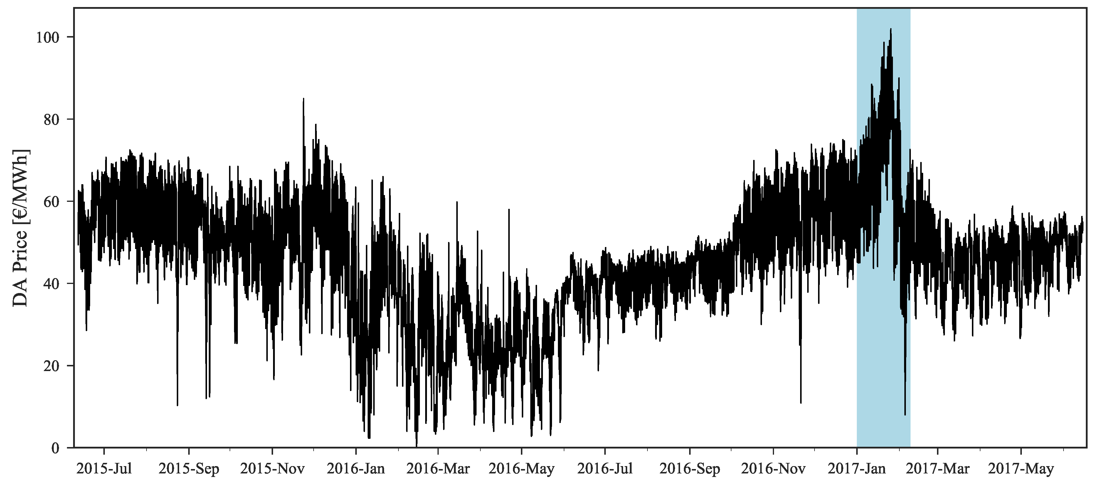
Figure 3.
Example of day-ahead and intraday hourly prices for the period between 14 and 15 July 2015.
Figure 3.
Example of day-ahead and intraday hourly prices for the period between 14 and 15 July 2015.

Figure 4.
Steps of the point and probabilistic price forecasting framework for the day-ahead market.
Figure 4.
Steps of the point and probabilistic price forecasting framework for the day-ahead market.

Figure 5.
Temporal framework of the short-term electricity price forecast.
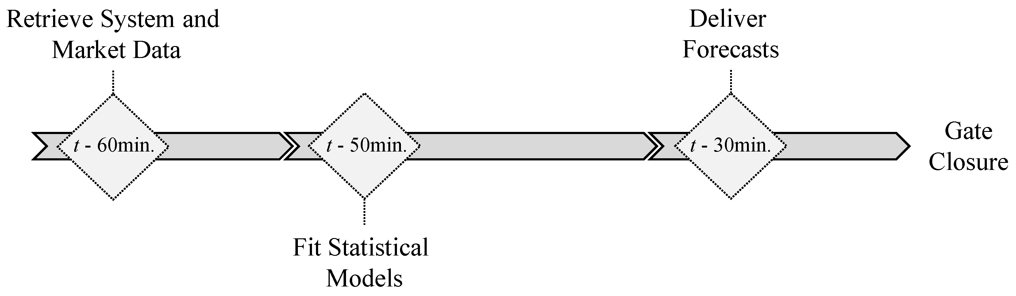
Figure 6.
Rolling window test procedure for day-ahead and intraday price forecasting skill evaluation. Dn () represents a specific day tested in the rolling window iterative process.
Figure 6.
Rolling window test procedure for day-ahead and intraday price forecasting skill evaluation. Dn () represents a specific day tested in the rolling window iterative process.

Figure 7.
Models’ improvement over the base model Mbase for mean absolute error (MAE), root mean square error (RMSE), mean absolute percentage error (MAPE) and continuous ranked probability score (CRPS) skill scores.
Figure 7.
Models’ improvement over the base model Mbase for mean absolute error (MAE), root mean square error (RMSE), mean absolute percentage error (MAPE) and continuous ranked probability score (CRPS) skill scores.

Figure 8.
Calibration (left) and sharpness (right) of probabilistic forecasts obtained with and without rescaling.
Figure 8.
Calibration (left) and sharpness (right) of probabilistic forecasts obtained with and without rescaling.

Figure 9.
Comparison of point and probabilistic forecast for low prices regime, with (bottom) or without (top) rescaling.
Figure 9.
Comparison of point and probabilistic forecast for low prices regime, with (bottom) or without (top) rescaling.

Figure 10.
Comparison of point and probabilistic forecast for medium prices regime, with (bottom) or without (top) rescaling.
Figure 10.
Comparison of point and probabilistic forecast for medium prices regime, with (bottom) or without (top) rescaling.

Figure 11.
Comparison of point and probabilistic forecast for high prices regime, with (bottom) or without (top) rescaling.
Figure 11.
Comparison of point and probabilistic forecast for high prices regime, with (bottom) or without (top) rescaling.
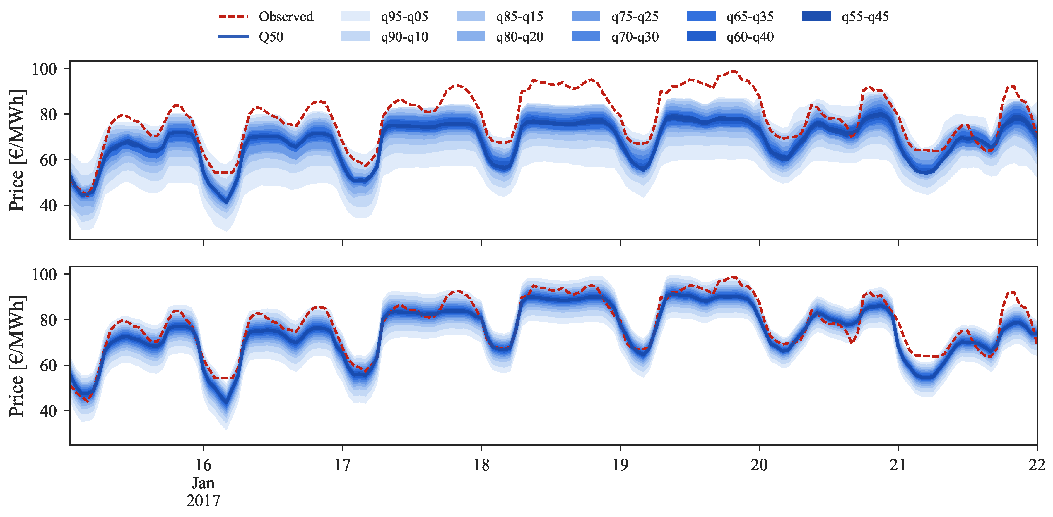
Figure 12.
Mean absolute error distribution for the test period: (a) original and (b) rescaled forecasts. The secondary yy axis shows the percentage of cases in each price interval forecasted by excess (overestimation) or deficit (underestimation) in relation to the observed price.
Figure 12.
Mean absolute error distribution for the test period: (a) original and (b) rescaled forecasts. The secondary yy axis shows the percentage of cases in each price interval forecasted by excess (overestimation) or deficit (underestimation) in relation to the observed price.
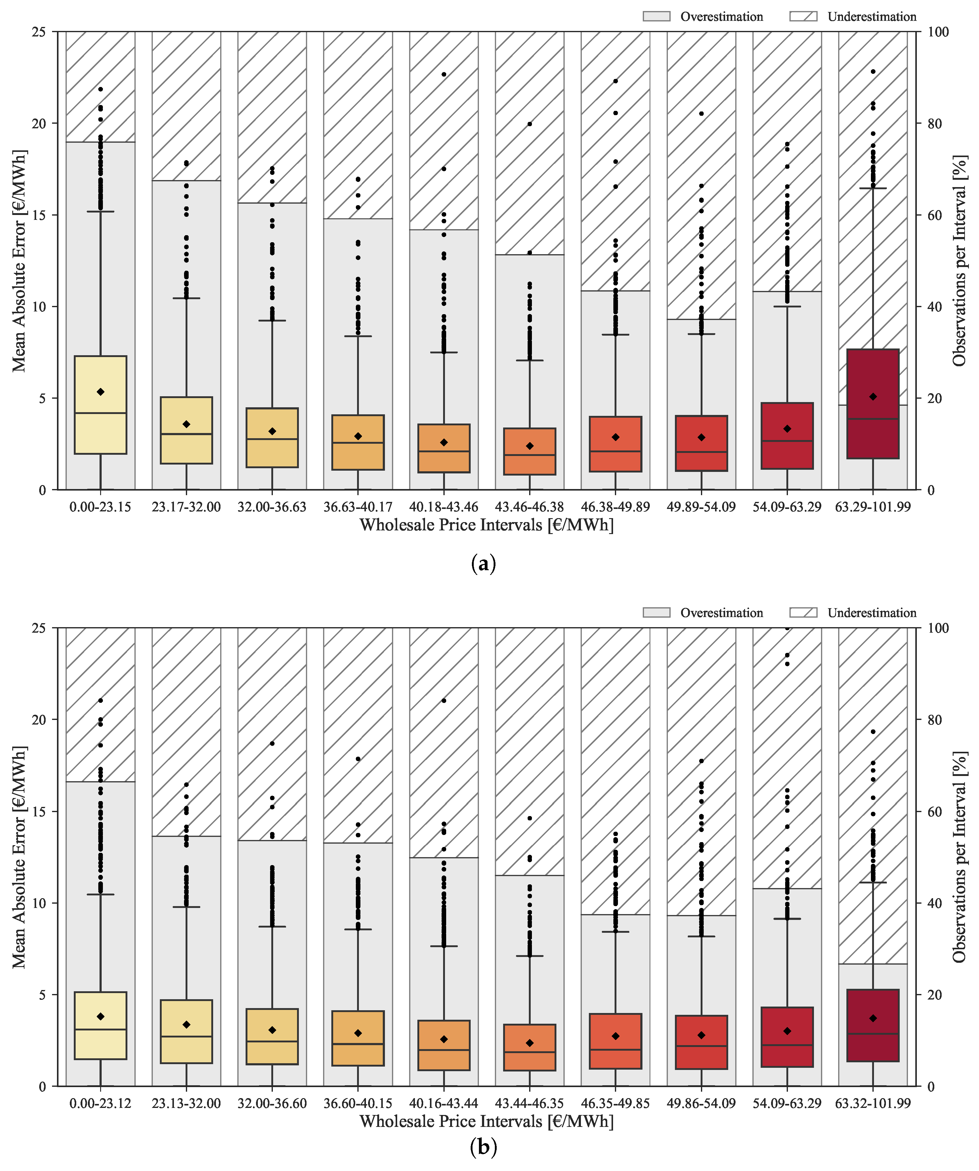
Figure 13.
Heatmap of mean absolute error calculated for the test period without rescaling (left) and with rescaling (right).
Figure 13.
Heatmap of mean absolute error calculated for the test period without rescaling (left) and with rescaling (right).

Figure 14.
Probabilistic forecast example for intraday (ID)1 (top) and ID2 (bottom) sessions.

Figure 15.
Probabilistic forecast example for ID3 (top) and ID4 (bottom) sessions.

Figure 16.
Probabilistic forecast example for ID5 (top) and ID6 (bottom) sessions.
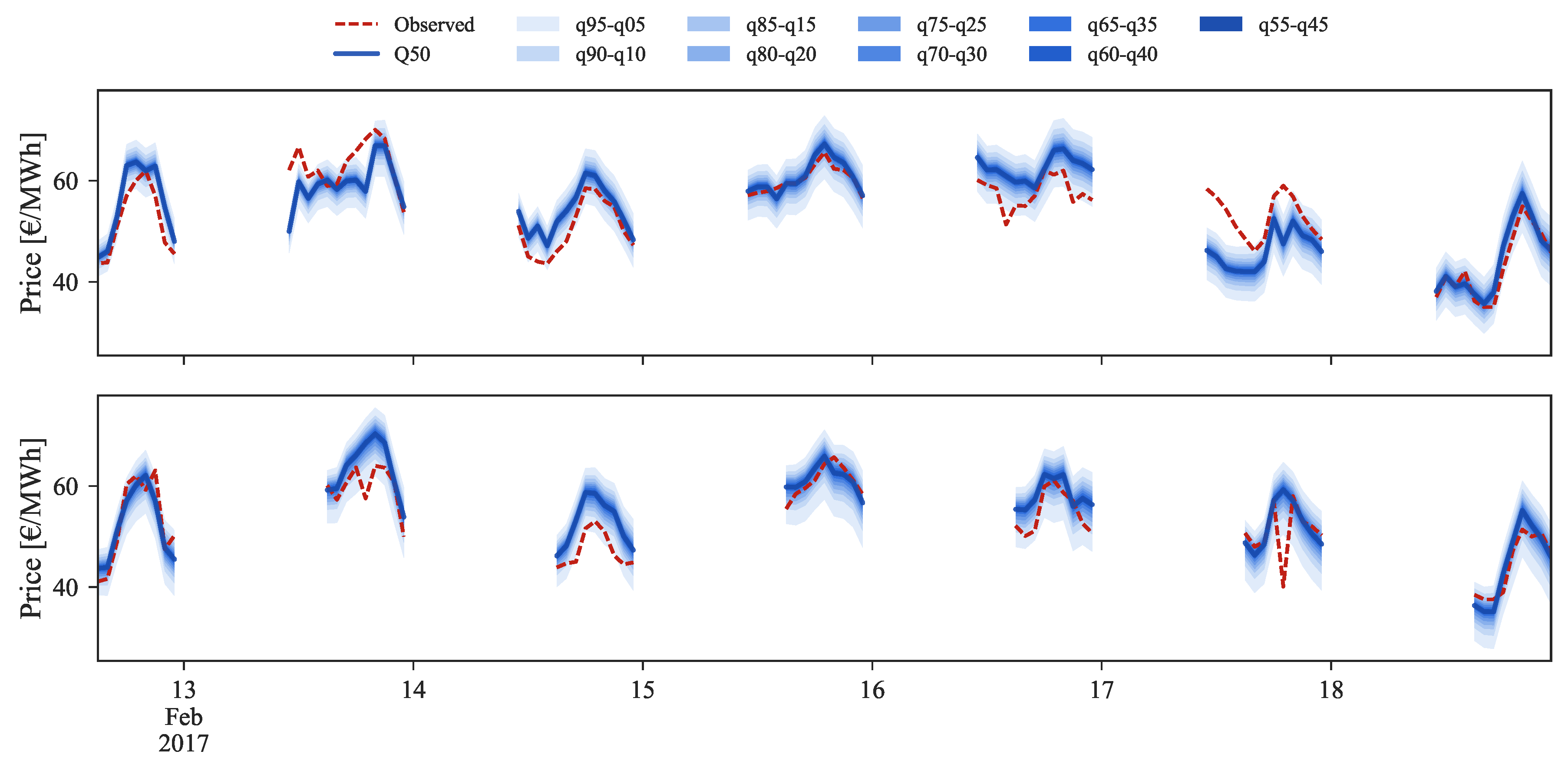
Figure 17.
Calibration and sharpness values of probabilistic forecasts for all intraday sessions.

Table 1.
Market data summary statistics.
| DA | ID1 | ID2 | ID3 | ID4 | ID5 | ID6 | ||
|---|---|---|---|---|---|---|---|---|
| Number of records | 17,616 | 19,815 | 17,616 | 14,680 | 12,476 | 9542 | 6606 | |
| Mean | €/MWh | 46.1 | 46.0 | 45.8 | 46.8 | 48.1 | 48.3 | 48.4 |
| Std. Deviation | €/MWh | 15.1 | 15.3 | 15.3 | 15.4 | 15.2 | 15.1 | 15.6 |
| Min | €/MWh | 0.0 | 0.0 | 0.0 | 0.0 | 0.0 | 0.0 | 0.0 |
| Max | €/MWh | 101.1 | 180.3 | 180.3 | 180.3 | 105.7 | 102.4 | 180.3 |
Table 2.
Available system variables for Portugal and Spain.
| Availability | ID | Variables | Country | Resolution |
|---|---|---|---|---|
| Historical () | P | Wholesale Electricity Price | PT | Hour |
| L | System Load | ES | Hour | |
| W | Wind Power Generation | PT, ES | Hour | |
| SPV | Photovoltaic (PV) Power Generation | ES | Hour | |
| ST | Solar Thermal Power Generation | ES | Hour | |
| CG | Cogeneration Generation | ES | Hour | |
| C | Coal Power Generation | ES | Hour | |
| CC | Combined Cycle Power Generation | ES | Hour | |
| FG | Fuel-Gas Power Generation | ES | Hour | |
| N | Nuclear Power Generation | ES | Hour | |
| HRC | Hydro Reservoir Capacity | PT, ES | Week | |
| HP | Hydro Reservoir Power Generation | PT, ES | Hour | |
| HRR | Hydro Run-river Power Generation | PT, ES | Hour | |
| HPSP | Hydro Pump Storage Power Generation | PT, ES | Hour | |
| NTC | Portugal-Spain NTC | PT, ES | Hour | |
| Future () | FPOMIP | Daily Price of Future Contracts (OMIP) | PT | Day |
| FL | System Load Forecasts | ES | Hour | |
| FLRes | Residual System Load Forecasts | ES | Hour | |
| FW | Wind Power Forecasts | ES | Hour | |
| FWPen | Wind Power Penetration Forecasts | ES | Hour | |
| FSPV | PV Forecasts | ES | Hour | |
| FST | Solar Thermal Forecasts | ES | Hour | |
| Calendar | CH | Hour of the Day [0, 23] | PT | - |
| CWd | Day of the Week [0, 6] | PT | - | |
| CM | Month of the Year [1, 12] | PT | - |
Table 3.
Individual impact of the most relevant variables in the forecasting skill of daily average price forecast.
Table 3.
Individual impact of the most relevant variables in the forecasting skill of daily average price forecast.
| Model | Variables | Evaluation Metrics | ||
|---|---|---|---|---|
| MAE | RMSE | MAPE | ||
| D_Base | CWd, CM, P | 3.92 | 5.21 | 10.54 |
| D_M1 | CWd, CM, P, FPOMIP | 2.32 | 3.15 | 6.76 |
| D_M2 | CWd, CM, P, FPOMIP, FW | 2.10 | 2.83 | 6.06 |
| D_M3 | CWd, CM, P, FPOMIP, FW, C | 2.07 | 2.79 | 6.02 |
| D_M4 | CWd, CM, P, FPOMIP, FW, C, W | 2.04 | 2.76 | 5.84 |
| D_Final | CWd, CM, P, FPOMIP, FW, C, W, SPV | 2.04 | 2.73 | 5.83 |
Table 4.
Forecasting skill results considering that each variable is individually added to the base model.
Table 4.
Forecasting skill results considering that each variable is individually added to the base model.
| Models | Evaluation Metrics | |||
|---|---|---|---|---|
| MAE | RMSE | MAPE | CRPS | |
| Error (Improvement) | Error (Improvement) | Error (Improvement) | Error (Improvement) | |
| B | 5.06 | 6.89 | 12.64 | 2.04 |
| B, FPOMIP | 3.98 (21.36%) | 5.45 (20.98%) | 10.29 (18.56%) | 1.60 (21.73%) |
| B, FWPen | 4.17 (17.56%) | 5.56 (19.30%) | 10.80 (14.55%) | 1.69 (17.18%) |
| B, FW | 4.24 (16.34%) | 5.71 (17.16%) | 10.86 (14.12%) | 1.71 (16.10%) |
| B, FLRes | 4.25 (16.00%) | 5.65 (18.03%) | 11.04 (12.71%) | 1.73 (15.40%) |
| B, FL | 5.04 (0.48%) | 6.80 (1.42%) | 12.71 (−0.52%) | 2.04 (0.06%) |
| B, HRC | 5.06 (−0.01%) | 6.92 (−0.41%) | 12.68 (−0.27%) | 2.046 (−0.33%) |
| B, C | 5.07 (−0.08%) | 6.81 (1.23%) | 12.69 (−0.36%) | 2.03 (0.50%) |
| B, SPV | 5.07 (−0.10%) | 6.91 (−0.25%) | 12.49 (1.22%) | 2.05 (−0.56%) |
| B, FSPV | 5.07 (−0.12%) | 6.90 (−0.15%) | 12.61 (0.25%) | 2.04 (−0.23%) |
| B, FST | 5.07 (−0.15%) | 6.87 (0.39%) | 12.64 (0.01%) | 2.04 (−0.10%) |
| B, ST | 5.08 (−0.27%) | 6.89 (0.09%) | 12.57 (0.55%) | 2.05 (−0.40%) |
| B, CG | 5.08 (−0.36%) | 6.93 (−0.56%) | 12.58 (0.51%) | 2.05 (−0.58%) |
| B, CC | 5.10 (−0.72%) | 6.94 (−0.60%) | 12.78 (−1.05%) | 2.05 (−0.65%) |
| B, FG | 5.10 (−0.72%) | 6.94 (−0.60%) | 12.78 (−1.05%) | 2.05 (−0.65%) |
| B, NTC | 5.10 (−0.74%) | 6.95 (−0.75%) | 12.70 (−0.42%) | 2.06 (−0.90%) |
| B, L | 5.11 (−0.85%) | 6.94 (−0.71%) | 12.68 (−0.28%) | 2.07 (−1.34%) |
| B, HPSP | 5.12 (−1.13%) | 6.951 (−0.83%) | 12.70 (−0.43%) | 2.06 (−1.28%) |
| B, HRR | 5.13 (−1.29%) | 6.975 (−1.17%) | 12.67 (−0.23%) | 2.08 (−1.95%) |
| B, N | 5.13 (−1.37%) | 6.94 (−0.67%) | 12.80 (−1.29%) | 2.08 (−1.78%) |
| B, W | 5.13 (−1.42%) | 6.97 (−1.16%) | 12.67 (−0.26%) | 2.07 (−1.64%) |
| B, HP | 5.14 (−1.58%) | 7.01 (−1.70%) | 12.74 (−0.81%) | 2.08 (−1.92%) |
Table 5.
Test combinations defined in the forward feature selection process. Mbase and Mfinal represent the baseline and the best selection of variables, respectively.
Table 5.
Test combinations defined in the forward feature selection process. Mbase and Mfinal represent the baseline and the best selection of variables, respectively.
| Model | Variables | ||||||||||||||||||||||||
|---|---|---|---|---|---|---|---|---|---|---|---|---|---|---|---|---|---|---|---|---|---|---|---|---|---|
| CH | CWd | CM | P | L | W | SPV | ST | CG | C | CC | FG | N | HRC | HP | HRR | HPSP | NTC | FPOMIP | FL | FLRes | FW | FWPen | FSPV | FST | |
| Mbase | x | x | x | x | |||||||||||||||||||||
| M1 | x | x | x | x | x | ||||||||||||||||||||
| M2 | x | x | x | x | x | x | |||||||||||||||||||
| M3 | x | x | x | x | x | x | x | ||||||||||||||||||
| M4 | x | x | x | x | x | x | x | x | |||||||||||||||||
| M5 | x | x | x | x | x | x | x | x | x | ||||||||||||||||
| M6 | x | x | x | x | x | x | x | x | x | x | |||||||||||||||
| M7 | x | x | x | x | x | x | x | x | x | x | x | ||||||||||||||
| M8 | x | x | x | x | x | x | x | x | x | x | x | x | |||||||||||||
| M9 | x | x | x | x | x | x | x | x | x | x | x | x | x | ||||||||||||
| M10 | x | x | x | x | x | x | x | x | x | x | x | x | x | x | |||||||||||
| M11 | x | x | x | x | x | x | x | x | x | x | x | x | x | x | x | ||||||||||
| M12 | x | x | x | x | x | x | x | x | x | x | x | x | x | x | x | x | |||||||||
| M13 | x | x | x | x | x | x | x | x | x | x | x | x | x | x | x | x | x | ||||||||
| M14 | x | x | x | x | x | x | x | x | x | x | x | x | x | x | x | x | x | x | |||||||
| M15 | x | x | x | x | x | x | x | x | x | x | x | x | x | x | x | x | x | x | x | ||||||
| M16 | x | x | x | x | x | x | x | x | x | x | x | x | x | x | x | x | x | x | x | x | |||||
| M17 | x | x | x | x | x | x | x | x | x | x | x | x | x | x | x | x | x | x | x | x | x | ||||
| M18 | x | x | x | x | x | x | x | x | x | x | x | x | x | x | x | x | x | x | x | x | x | x | |||
| M19 | x | x | x | x | x | x | x | x | x | x | x | x | x | x | x | x | x | x | x | x | x | x | x | ||
| M20 | x | x | x | x | x | x | x | x | x | x | x | x | x | x | x | x | x | x | x | x | x | x | x | x | |
| M21 | x | x | x | x | x | x | x | x | x | x | x | x | x | x | x | x | x | x | x | x | x | x | x | x | x |
| Mfinal | x | x | x | x | x | x | x | x | x | x | x | ||||||||||||||
Table 6.
Forecasting skill evaluation of the rescaling process.
| Models | Forecast Evaluation Metrics | |||
|---|---|---|---|---|
| MAE | RMSE | MAPE | CRPS | |
| Error (Imp.) | Error (Imp.) | Error (Imp.) | Error (Imp.) | |
| Mfinal | 3.42 | 4.63 | 8.97 | 1.39 |
| Mrescaled | 3.06 (10.32%) | 4.09 (11.58%) | 8.61 (3.99%) | 1.27 (8.80%) |
| Mrescaled, {FL} | 3.06 (10.43%) | 4.09 (11.73%) | 8.62 (3.89%) | 1.24 (10.55%) |
| Mrescaled, {FL, FWPen} | 3.03 (11.20%) | 4.04 (12.61%) | 8.54 (4.75%) | 1.22 (12.58%) |
Table 7.
Forecast results for the intraday market sessions.
| (a) Intraday 1 (ID1) | ||||
| Model | Forecast Evaluation Metrics | |||
| MAE | RMSE | MAPE | CRPS | |
| IM1 | 1.96 | 2.96 | 5.64 | 0.82 |
| IM2 | 1.95 | 2.97 | 5.63 | 0.82 |
| IM3 | 1.94 | 2.95 | 5.59 | 0.84 |
| (b) Intraday 2 (ID2) | ||||
| Model | Forecast Evaluation Metrics | |||
| MAE | RMSE | MAPE | CRPS | |
| IM1 | 1.74 | 2.72 | 5.22 | 0.74 |
| IM2 | 1.74 | 2.72 | 5.21 | 0.74 |
| IM3 | 1.73 | 2.73 | 5.21 | 0.77 |
| IM4 | 1.73 | 2.72 | 5.20 | 0.76 |
| (c) Intraday 3 (ID3) | ||||
| Model | Forecast Evaluation Metrics | |||
| MAE | RMSE | MAPE | CRPS | |
| IM1 | 1.74 | 2.80 | 5.07 | 0.74 |
| IM2 | 1.74 | 2.81 | 5.03 | 0.74 |
| IM3 | 1.74 | 2.82 | 5.05 | 0.77 |
| IM4 | 1.74 | 2.81 | 5.05 | 0.76 |
| (d) Intraday 4 (ID4) | ||||
| Model | Forecast Evaluation Metrics | |||
| MAE | RMSE | MAPE | CRPS | |
| IM1 | 1.59 | 2.95 | 4.32 | 0.70 |
| IM2 | 1.58 | 2.95 | 4.31 | 0.69 |
| IM3 | 1.58 | 2.95 | 4.34 | 0.71 |
| IM4 | 1.58 | 2.92 | 4.36 | 0.70 |
| (e) Intraday 5 (ID5) | ||||
| Model | Forecast Evaluation Metrics | |||
| MAE | RMSE | MAPE | CRPS | |
| IM1 | 1.96 | 3.01 | 5.39 | 0.83 |
| IM2 | 1.95 | 3.00 | 5.34 | 0.82 |
| IM3 | 1.93 | 2.98 | 5.38 | 0.83 |
| IM4 | 1.92 | 2.93 | 5.33 | 0.82 |
| (f) Intraday 6 (ID6) | ||||
| Model | Forecast Evaluation Metrics | |||
| MAE | RMSE | MAPE | CRPS | |
| IM1 | 2.56 | 4.38 | 6.65 | 1.07 |
| IM2 | 2.55 | 4.38 | 6.64 | 1.08 |
| IM3 | 2.53 | 4.37 | 6.61 | 1.07 |
| IM4 | 2.54 | 4.37 | 6.64 | 1.06 |
© 2017 by the authors. Licensee MDPI, Basel, Switzerland. This article is an open access article distributed under the terms and conditions of the Creative Commons Attribution (CC BY) license (http://creativecommons.org/licenses/by/4.0/).
Share and Cite
MDPI and ACS Style
Andrade, J.R.; Filipe, J.; Reis, M.; Bessa, R.J. Probabilistic Price Forecasting for Day-Ahead and Intraday Markets: Beyond the Statistical Model. Sustainability 2017, 9, 1990. https://doi.org/10.3390/su9111990
AMA Style
Andrade JR, Filipe J, Reis M, Bessa RJ. Probabilistic Price Forecasting for Day-Ahead and Intraday Markets: Beyond the Statistical Model. Sustainability. 2017; 9(11):1990. https://doi.org/10.3390/su9111990
Chicago/Turabian StyleAndrade, José R., Jorge Filipe, Marisa Reis, and Ricardo J. Bessa. 2017. "Probabilistic Price Forecasting for Day-Ahead and Intraday Markets: Beyond the Statistical Model" Sustainability 9, no. 11: 1990. https://doi.org/10.3390/su9111990
Note that from the first issue of 2016, this journal uses article numbers instead of page numbers. See further details here.