Assessing the Bicycle Network in St. Louis: A PlaceBased User-Centered Approach

Abstract

To transition towards sustainability and increase low-impact transportation, city planners are integrating bicycle infrastructure in urban landscapes. Yet, this infrastructure only promotes cycling according to how well it is sited within a specific city. How to best site bicycle facilities is essential for sustainability planning. We review approaches to assessing and siting new bicycle facilities. Following sustainability science, we argue that active cyclists should be consulted to incorporate users’ site-specific knowledge into bicycle infrastructure assessments. We then pilot an approach that surveys cyclists concerning level of stress along routes ridden in St. Louis, MO, USA. Among the active cyclists surveyed (n = 89), we found stress correlates with speed limit, roadway classification, and number of lanes. Although cyclists surveyed in St. Louis prefer roads with bike lanes over roads with sharrows or no infrastructure, the presence of bicycle infrastructure had no correlation with reported levels of stress. The piloted survey and spatial analytic tool are transferable to other localities. For planners, the maps generated by this participant data approach identify high-stress routes as targets of new infrastructure or information to direct cyclists to safer routes. For bicyclists, the maps generated identify low-stress routes for recreation and commuting.

1. Introduction

In sustainability planning, cities are working to increase bicycle-use due to the social, environmental, and economic benefits of bicycle commuting. The physical activity involved in active commuting can help reduce morbidity risk of many health conditions, such as cardiovascular disease [1,2], obesity [3,4], and diabetes [5,6]. It can improve overall physical health [7,8] as well as mental health [9,10]. Cycling that replaces automobile trips results in reduced greenhouse gas emissions and decreased consumption of natural resources [11,12] helping cities achieve air quality standards. Economic benefits for bicycle commuters include savings on gasoline and parking fees. When cycling replaces car ownership altogether, possible savings are even greater, as the average annual cost of owning and operating a mid-sized sedan in the United States is $8716 USD [13]. Cities with higher rates of bicycle commuting benefit from reduced vehicle congestion on roads and parking lots as well as reduced wear on street surfaces. The economic benefits of bicycle commuting have potential to serve as a stimulus for local economies [14]. Due to the benefits, cities are exploring techniques to increase their transportation mode share of bicycle commuters.

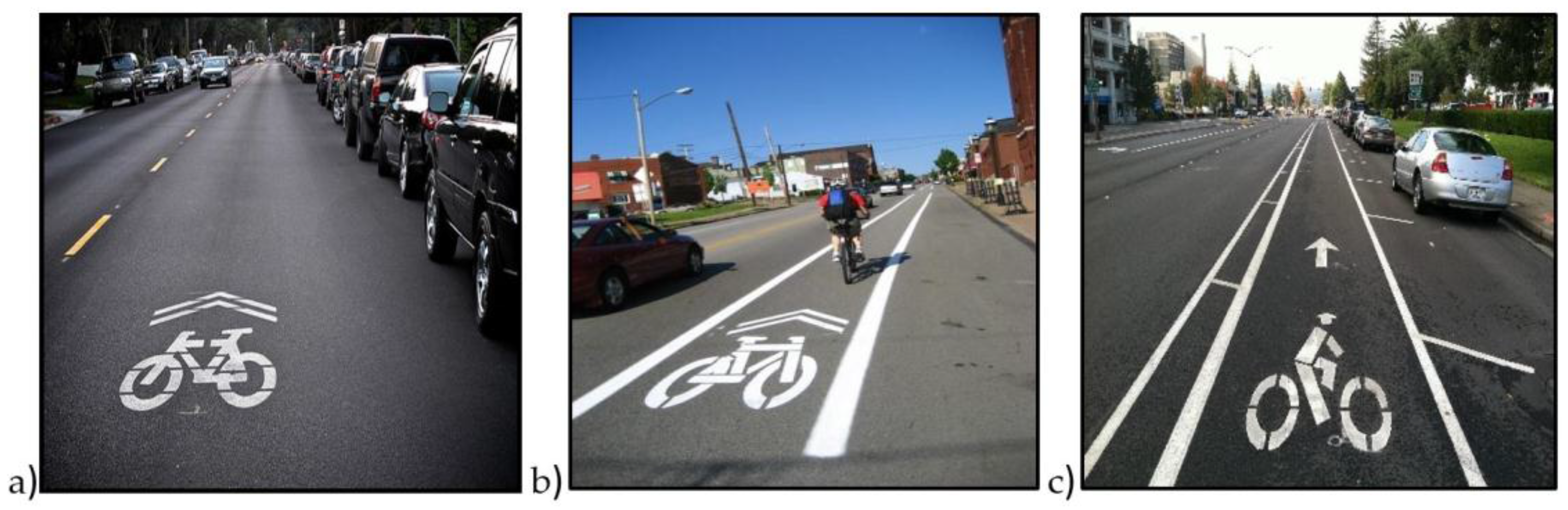
Urban planners can facilitate cycling by incorporating bicycle infrastructure into street networks. Common infrastructure types include shared-use lane markings or “sharrows”, on-street painted bike lanes, and buffered bike lanes which provide extra segregation from traffic (Figure 1).

The value of such infrastructure for increasing cycling is mixed. While many studies have found a positive correlation between levels of bicycle infrastructure and bicycle commuting [15,16,17] others have found little correlation [18,19,20,21]. What is certain is that many cyclists prefer routes with bicycle facilities [22,23,24,25,26,27,28] and bicycle infrastructure encourages non-cyclists to try cycling [14]. However, it is uncertain whether investments in bicycle infrastructure increase bicycle-use.

Expensive public tax-funded infrastructure projects can be contentious among citizens and local officials. Therefore, it is important that cities assess the quality of their bicycle infrastructure with respect to meeting cyclists’ needs. This paper seeks to inform development of urban bicycle infrastructure policy that can transition society towards sustainability. Using sustainability science as a framework for generating usable knowledge [29,30], we argue that empirically-driven approaches relying on site-specific and user-centered data [31,32] offer alternative means of matching infrastructure with cyclists riding preferences. First we review instruments for evaluating bicycle networks. Then describe a user-centered approach we implemented in St. Louis. We discuss the results of the study and both its advantages and limitations. Finally, we discuss how cyclists’ preferences for routes and route characteristics in a specific locale can inform city planners and bicycle network users.

2. Audit Instruments for Bicycle Networks

There are several approaches for auditing and assessing bicycle infrastructure. Most provide an account of a study site’s entire bicycle network including bicycle facilities, roads, and paths. Landis, Venkat, and Brannick [33] developed the Bicycle Level of Service (BLOS) method, used in the Highway Capacity Manual (HCM), a standard for transportation planning throughout much of the U.S. Harkey, Reinfurt, and Knuiman, with the U.S. Federal Highway Administration (FHWA), later formulated the Bicycle Compatibility Index (BCI) [34]. Both methods use a catalog of measurable traffic and roadway characteristics—such as roadway width, pavement surface condition, and motor vehicle speed—to assess all segments of a network. Segments are then given a letter grade “A” through “F” by how closely they meet BCI and BLOS standards (see Moudon & Lee [35] for a review of 11 closely related bicycle network audit instruments). One critique of these methods is that due to the extensive amount of variables used, results have little actionable meaning to either planners or users of the network [36,37,38]. For example, it is difficult to conceptualize the difference between two letter grades, such as an “A” segment and a “B” segment.

An alternative method is to rate segments by a single indicator. Many studies have found that one of the greatest impediments to cycling is the perceived danger from motor traffic [39,40,41]. Based on this concept and earlier studies [24,42], Mekuria et al. [38] developed the Level of Traffic Stress (LTS) assessment method. The LTS method assesses network segments based on the amount of stress put on cyclists as a result of the environmental characteristics present. Using predetermined criteria, each segment of the network is given an LTS rating from 1 to 4, resulting in a map that shows which route segments are appropriate for cyclists of different confidence levels. Because segments are measured by stress alone, results from LTS studies are more easily understood by users, cyclists, and planners.

A criticism of many bicycle network audit instruments is that the criteria and standards are developed a priori with standards imported from places outside of the locale in question. For example, the LTS method used by Mekuria et al. [38] in San Jose, CA, USA, is based on bicycle facility planning and design standards from The Netherlands. This constrains planning as bicycle culture, city structure, traffic patterns, as well as motorist and cyclist behavioral norms can differ widely from location to location. To illustrate this concept, Chataway, Kaplan, Nielsen, and Prato [43] compared perceptions of bicycle infrastructure between cyclists from Brisbane, Australia, and Copenhagen, Denmark, and found that when presented with the same generic infrastructure layouts, cyclists from Brisbane perceived them as less safe than cyclists from Copenhagen. Heinen and Handy [44] interviewed both cyclists and non-cyclists from Davis, California, and Delft, The Netherlands, and found that participants from Davis viewed bicycle commuting as unsafe to a greater extent than participants from Delft, even though both are considered very bicycle-friendly cities with extensive bicycle infrastructure and policies in place [44]. These examples illustrate the differing perceptions of cycling and cycling safety across locations, limiting the transferability of research instruments across study sites.

A more accurate assessment of a bicycle network would come from the cyclists who use the network, as they are tacitly familiar with the network, traffic patterns, and with how cycling fits within that particular culture and environment. Data from local cyclists have been produced through other study models, such as bicycle route choice (BRC) studies cf. [45,46]. These studies identify and examine routes chosen by cyclists and use statistical analyses to infer cyclists’ preferences for bicycle infrastructure and other route characteristics. Because BRC studies include an analysis of route segments, they could also be used as a network assessment tool. Data gathered are user-centric and place-specific, so results more accurately reflect nuances of focal locales. The following section reviews different BRC models to show the progression of this method and suggest how it could be used as a network assessment tool.

3. Bicycle Route Choice Studies

BRC studies use either stated preference or revealed preference models to collect data. Stated preference methods include surveys or focus groups where participant cyclists are presented with different route segment characteristics (e.g., speed limit, traffic volume, and presence of bicycle facilities) and are asked about their preferences for each [46,47,48,49]. Some studies include hypothetical scenarios, such as biking to work or an all-day meeting [25,50]. Results are then analyzed using statistical models to measure cyclists’ stated preferences for certain route characteristics. While these studies can produce valuable data about cyclists’ preferences, they do not necessarily provide an assessment of a particular bicycle network. Further, these studies are based on hypothetical data and fictional scenarios which may not translate accurately to the real world.

BRC studies that utilize revealed preference methods are based on either cyclist recall data or real-time data produced through GPS. These spatially-explicit studies often ask participants to draw out recent or commonly-used bike routes within a study area on a paper map or website [24,26,28,51]. Researchers then use these documented routes and statistical analyses to make inferences about cyclists’ preferences for network characteristics. Some compare actually used routes to shortest possible routes based on start and end positions [27,52]. More recent studies have equipped participants with GPS units to collect data on travel behavior and routes used [22,27,52,53]. Using GPS data is beneficial, as it is based on actual cycling behavior and simplifies the digitization process into GIS analytic software (ESRI: Redlands, CA, USA). This approach is disadvantaged by higher research costs and the requirements of greater participant involvement.

Rather than simply analyzing routes used by cyclists, other BRC studies have collected feedback from participants about their routes. Krykewycz et al. [37] used crowdsourcing to collect user feedback on points throughout a bicycle network. Snizek et al. [28] used a website to allow participants to place points of positive or negative experiences along their routes. However, the authors noted that simple positive and negative measurements can be ambiguous to planners and users of a network.

Similarly, Howard and Burns [24] asked participants to rate their routes from 1–5 based on the level of stress they felt while cycling on traveled routes. Results produced stress measurements for entire routes [24]. While these are useful for larger-scale bicycle network characterizations, they are less meaningful to decision makers deciding how to invest limited funds in bicycle infrastructure. In the following section, we adapt the above approaches to pilot a network assessment tool that incorporating riders’ level of stress measurements at finer spatial scales; scales more useful to decisions makers and riders.

4. Methods

This study utilized user-centric data acquired through a BRC study model to perform a bicycle network assessment of segments within a study area in St. Louis, MO, USA. We collected data from cyclists to produce level of traffic stress (LTS) measurements for each route segment ridden within the study area. Analysis reveals local cyclists’ preferences for routes, bicycle infrastructure, and other environmental characteristics. The resulting composite map has potential to be used by local cyclists looking for low-stress routes and by city officials and planners of future bicycle infrastructure looking to reduce high stress segments for cyclists.

4.1. Study Area

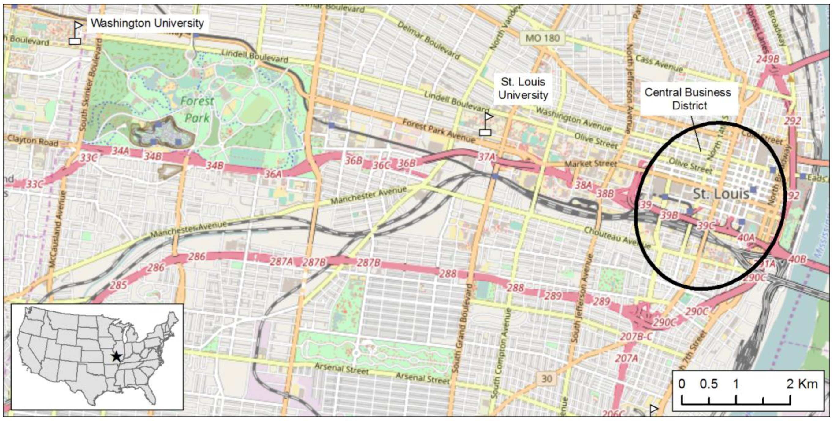
In 2004, the City of St. Louis, MO, USA (Figure 2) partnered with local non-governmental organization Great Rivers Greenway to create the Bike St. Louis Network which connects different parts of the city. In support of this program, both St. Louis City and St. Louis County have been adding bicycle infrastructure to the local street network. By the end of Phase III in 2015, the total amount of on-street bicycle routes was 217 km [54]. Bicycle facilities analyzed in this project include sharrows, bike lanes, and buffered bike lanes.

To explore the development of a network assessment approach, we narrowed the study area to the central corridor from eastern St. Louis County to downtown St. Louis City which is among the most highly used corridors by all forms of transportation in the region (Figure 2). The study area included two large universities, Washington University and Saint Louis University, and covered 9 of the 10 road segments most used by cyclists according to the 2014 Great Rivers Greenway Bicycle Count Report [55].

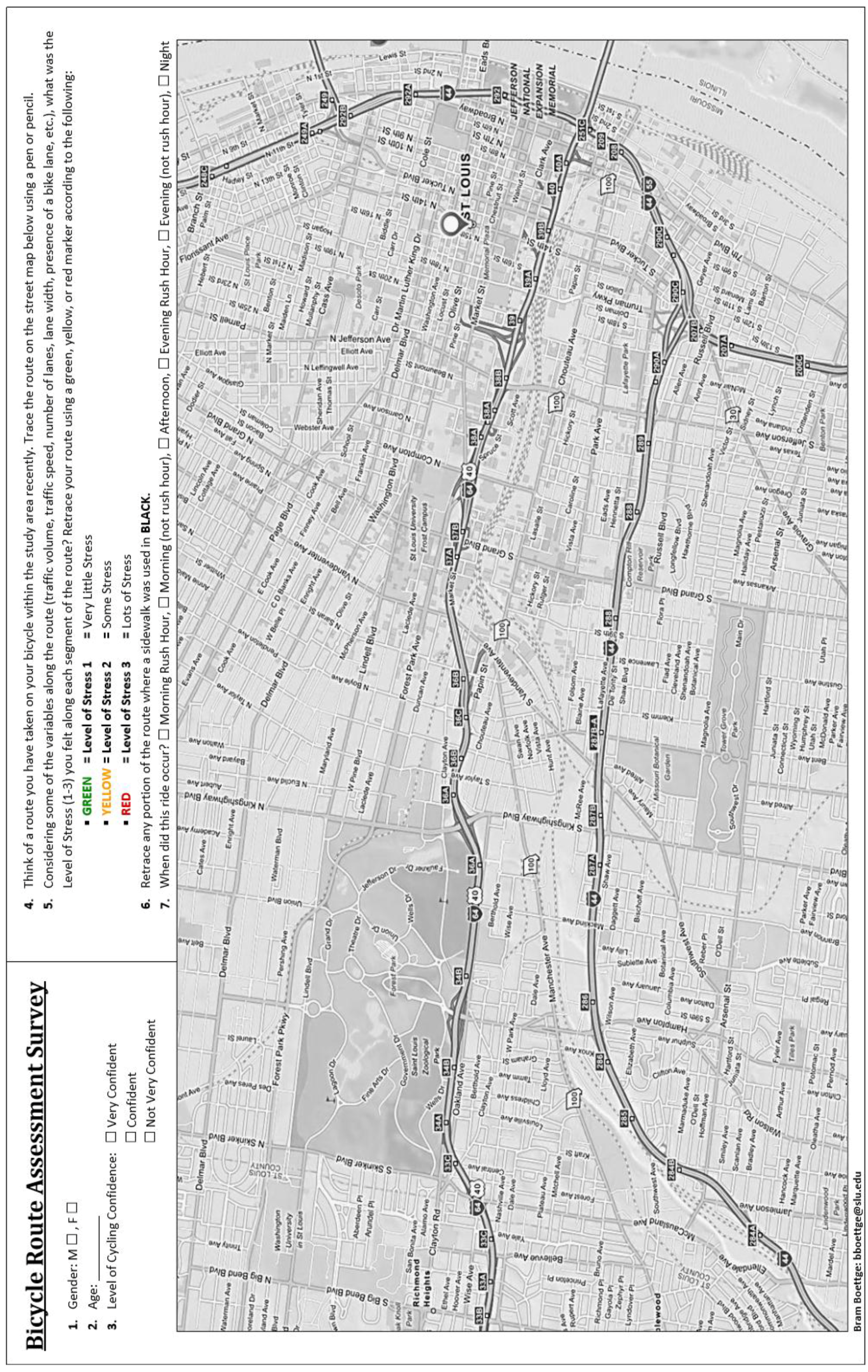
4.2. Survey Instrument

The study utilized a paper-based survey administered in person (Appendix A) (Saint Louis University Institutional Review Board approval #26086). Benefits to in-person surveys are that participants are able to ask questions and surveyors can oversee survey completion cf. [31,32]. Surveys were printed on A3 sized paper (11” × 17”), and contained demographic questions, a street map of the study area, and instructions for identifying routes.

Participants were asked to designate their level of cycling confidence, whether they were very confident, confident, or not very confident adapted from [56]. Participants were also asked to draw out a bike route they had used recently on the study area map using a pencil and then to retrace their route, using green, yellow, and red markers, with defined colors designating the level of stress they felt on each segment of the route. The color red implied lots of stress (LTS = 3), yellow some stress (LTS = 2), and green very little stress (LTS = 1). Participants were instructed to consider the variables traffic volume, traffic speed, number of lanes, lane width, and presence of bicycle facilities when reporting route segment stress levels. Participants rated each segment of their route according to their own perceptions of stress, given the provided stress level definitions. Participants were then asked to use a black marker on segments where a sidewalk was used. It is illegal to use a bicycle on many sidewalks within the study area, so for the purposes of this study, they were not considered part of the bicycle network. Participants were also asked to mark what time of day they rode this route morning rush hour, morning not rush hour, afternoon, evening rush hour, evening not rush hour, or night (Appendix A).

4.3. Participant Recruitment

Surveys were distributed by two methods for six weeks from August to September of 2015. We established booths at four local cycling events hosted by Saint Louis University and Trailnet, a local bicycle advocacy organization. Participants were recruited to voluntarily complete the survey in person and on site. Persons over the age of 18 who had recently ridden a bicycle on the streets within the study area were allowed to participate in the survey. The study did not differentiate between bicycle commuters and recreational cyclists, as both are considered users of the bicycle network and are equally affected by the environmental variables along their routes.

In total, 89 surveys were completed and used in the study. Sixty-three participants were male, representing 70.8% of the total (

Table 1. Participant demographics.

Group	Number	%
Gender
Male	63	70.8
Female	26	29.2
Age
Mean	40.4
Median	37.5
Level of Cycling Confidence
Very Confident	49	55.1
Confident	37	41.6
Not Very Confident	2	2.2

). While inconsistent with the total population of adult bike riders in the U.S., which is 54% male [55], the sample is consistent with the percentage of male cyclists found in a previous St. Louis study [57] as well as in national bike commuting statistics [58].

Most participants, 49 (55%), responded that they were very confident, while 37 (41.6%) were confident. This was expected, as most participants were recruited at bicycling events. Results therefore will reflect the opinions of very confident or confident cyclists. This reported cycling confidence suggests that participants were likely experienced cyclists, capable of providing accurate assessments of their routes.

4.4. Route Segment Data Capture

Each hand-drawn route was digitized using ArcGIS 10.3.1 software (ESRI: Redlands, CA, USA) by selection of visually corresponding street segments in a high quality digital street file. For each participant route, we merged component segments into a single GIS polyline route. We then split the polyline where the designated levels of stress changed from one level to another and added corresponding LTS values to the attribute table for each segment. Attribute values for gender, age, and level of cycling confidence were also entered for each segment. We note that among the 89 routes, there were multiple shared route segments among participant routes.

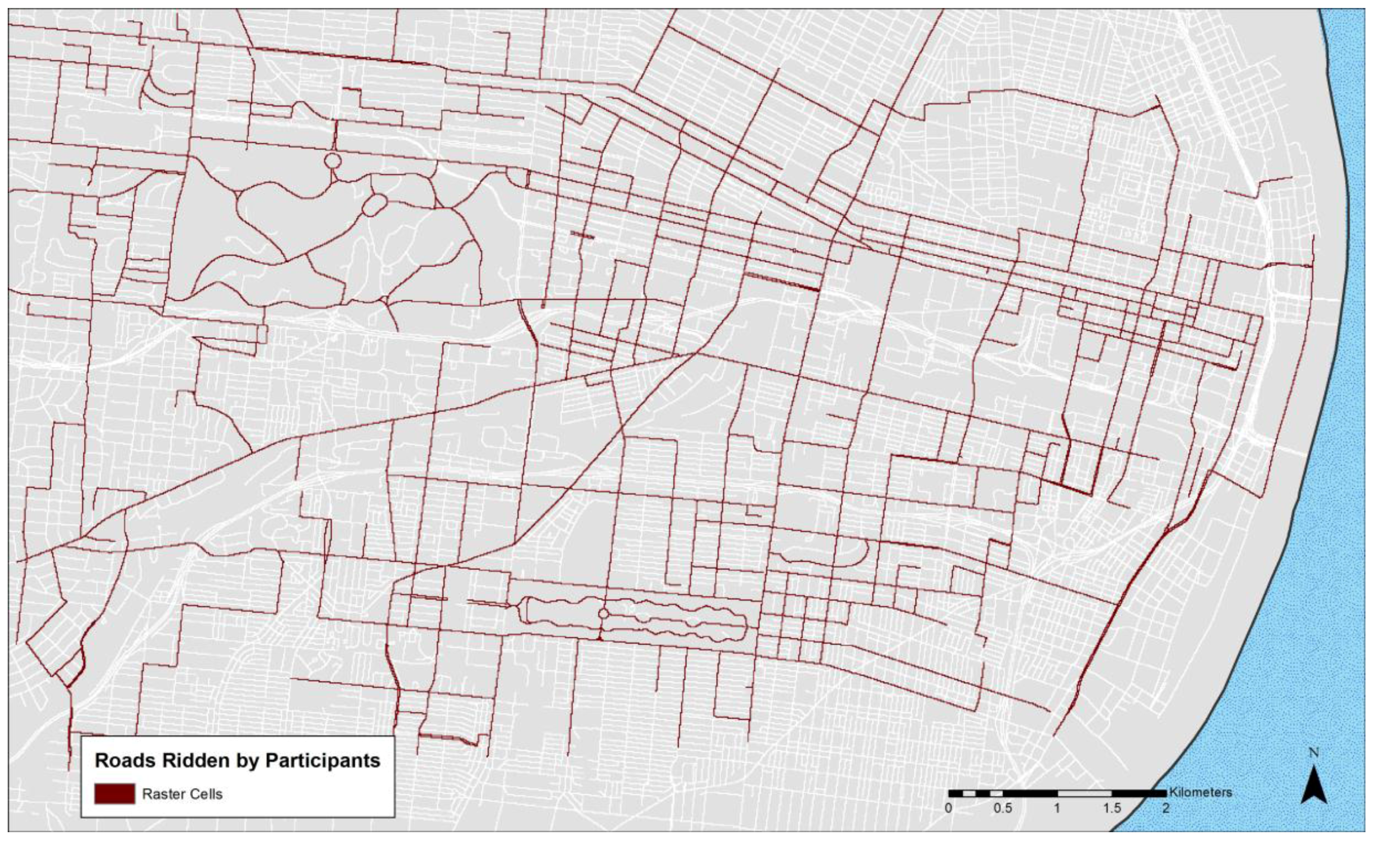
For data visualization and analysis, we combined all routes into a single GIS layer. To do so, we first converted each participant route from vector polyline to gridded raster format using a cell size of 10 m yielding 89 individual raster layers of routes containing LTS values at the pixel level. We then combined all 89 rasterized routes into a single composite layer via raster overlay. For each pixel, variables quantifying the mean LTS value and the number of participants reporting the pixel location as part of their route were generated. There were 33,500 cells present in this composite layer representing routes identified by participants. Cells reported by only one participant were excluded, yielding 18,760 cells (56%) that were used for analysis ( see Figure 3).

Cells included for analysis were converted to vector points (i.e., cell x,y centers). This enabled the use of an ArcGIS data extraction tool to extract from each cell the mean LTS values and number of reporting cyclists to a vector point file with a corresponding attribute table comprised of records in a standard tabular database format. The unit of observation was an individual point located on a route reported by at least two participants. The now tabular data was in a format amenable to analysis using SPSS statistical software (IBM: Armonk, NY, USA).

4.5. Environmental Co-Variates

Following other BRC studies [22,24,26,27,28,50,51,52], we included the following environmental variables in our statistical analysis: street functional classification, traffic speed, number of lanes, and bicycle facility type. Environmental data were tagged to each individual data point. Data for traffic volume were unavailable, so as an alternative we used street functional classification data which categorize all road segments as local, minor collectors, major collectors, minor arterials, or principal arterials. These data are more widely available and often used to categorize traffic intensity [22,27,28,38]. Based on the FHWA definitions of urban functional classifications summarized in

Table 2. Summaries of functional classification definitions according to the U.S. Federal Highway Administration (FHWA) (2013) [59].

Functional Classification	FHWA Definitions
Principal Arterials	Serve major activity centers, highest traffic volume corridors and longest trip demands
	Carry high proportion of total urban travel on minimum of mileage
Minor Arterials	Interconnect and augment the higher level Arterials
	Serve trips of moderate length at a somewhat lower level of travel mobility than Principal Arterials
Major Collectors	Serve both land access and traffic circulation in higher density residential, and commercial/industrial areas
	Operating characteristics include higher speeds and more signalized intersections
Minor Collectors	Serve both land access and traffic circulation in lower density residential and commercial/industrial areas
	Operating characteristics include lower speeds and fewer signalized intersections
Local Roads	Carry no through traffic movement
	Constitute the mileage not classified as part of the Arterial and Collector systems

, we assume traffic intensity to be high for arterial roads, medium for collectors, and low for local roads. We captured number of lanes from Google imagery.

We were able to acquire GIS shapefiles for speed limit, functional classification, and bicycle facilities. However, they were not perfectly aligned with our GIS files of participant routes. Due to the volume of data points involved, the task of spatial alignment was time prohibitive. To expedite the process while maintaining statistically validity, we generated a random sample of 200 points from the existing 18,761 points. Data were manually entered for all 200 points.

4.6. Statistical Analysis Methods

To measure the effect that bicycle infrastructure and other environmental variables had on where participants chose to ride and the levels of stress they felt, we used descriptive statistics (

Table 3. Descriptive statistics for avgLTS and Number of Times Ridden (NTR).

Statistic	avgLTS	NTR
Number	200	200
Range	1.667	20.00
Minimum	1.000	2.000
Maximum	2.667	22.000
Mean	1.515	4.475
Median	1.429	3.000
Mode	1.000	2.000
Standard Deviation	0.485	3.308
Variance	0.235	10.944
Skewness	0.658	2.488
Kurtosis	−0.597	7.556

) and statistical analysis from our 200 data points. We used the dependent variables average level of traffic stress (avgLTS) and number of times ridden (NTR), and the independent variables speed limit, functional classification, number of lanes, and bicycle facility type.

Because avgLTS and NTR data were not normally distributed and ordinal in nature, we used a comparison of medians and Kruskal-Wallis H tests to test if median avgLTS and NTR scores were significantly different across the different group categories of the independent variables. Kruskal-Wallis H tests do not require data to be normally distributed and allow median values to be compared among groups. A caveat to our statistical analysis was that the avgLTS data violated the assumption of independence of observations (data should be independent of each other and such that no two data points should contain responses from the same participant). Since the avgLTS variable was made up of an average of LTS ratings from multiple participants, it is likely that the ratings from the same participant were included in more than one of the 200 sample point observations.

The formula for the Kruskal-Wallis H test is:

$$H=\frac{12}{n\left(n+1\right)}{\displaystyle \sum }_{i=1}^k\frac{R_i^2}{n_i}-3\left(n+1\right)$$

where H equals the test statistic, n equals the number of observations in all samples, and R_i equals the sum of the mean ranks assigned to each group. Results from H tests only indicate that at least one of the median values among the different groups within an independent variable is significantly statistically different. To find out which specific groups were significantly different from each other, we performed pairwise comparisons using Dunn’s (1964) procedure with a Bonferroni correction for multiple comparisons. Results from these tests allow interpretation of whether the different categories of independent variables had an effect on where cyclists chose to ride and the level of stress they felt while riding.

5. Results

The methods from this study were designed to use locally-derived data to assess the bicycle network of a specified area of St. Louis. The assessment focused on where participant cyclists chose to ride within the study area, the level of stress they felt while riding, and how these were influenced by the bicycle infrastructure available and environmental conditions.

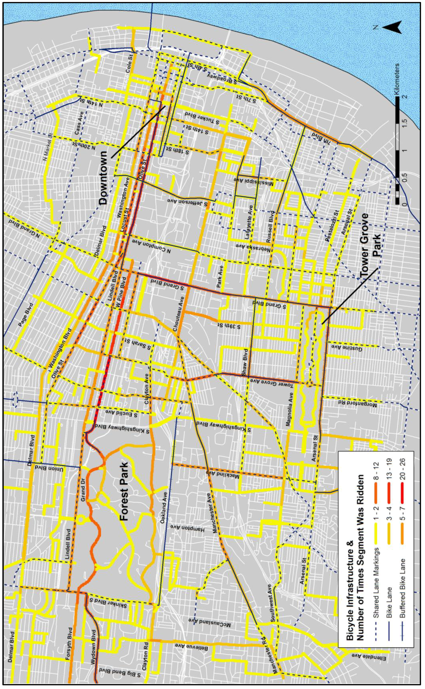
5.1. Visual Analysis of Number of Times Ridden (NTR)

Figure 4 shows the number of times each road segment within the study area was ridden by participants and the available bicycle infrastructure. As expected, the roads most heavily used by participants run east and west along the central corridor between central St. Louis County and Downtown St. Louis. Roads running north and south were used less often. In general, local roads and roads farther away from the central corridor were also used less often. Bicycle infrastructure is well dispersed. Sharrows are the most abundant facility type, while buffered bike lanes are the scarcest. The map shows that many participants chose roads with bicycle facilities.

Figure 4 also allows for comparisons of parallel roads that offer different types of bicycle facilities. Many of these occurrences show that cyclists chose roads with bike lanes over roads with sharrows but chose roads with sharrows over roads with no infrastructure at all. One example is where Washington Avenue, Locust Street, and Olive Street run parallel just west of Downtown. Olive Street contains a bike lane and was the most heavily used of the three parallel streets.

5.2. Visual Analysis of Average Level of Traffic Stress (avgLTS)

Figure 5 shows avgLTS values for all roads used by participants and the bicycle infrastructure available. In general, local roads seemed to receive lower avgLTS scores compared to collector and arterial roads, and the Downtown area appears to have higher avgLTS scores than other areas. Many of the roads running north and south through the central corridor received higher stress scores compared to roads running east and west.

Looking at parallel roads that offer different types of bicycle facilities in Figure 5, associations between bicycle infrastructure and avgLTS are less consistent, though there are several occurrences where roads with bicycle lanes have higher avgLTS values than roads with sharrows or no infrastructure. Focusing on the same location as in the section above, we find an example of this where Washington Avenue, Locust Street, and Olive Street run parallel just west of Downtown. Olive Street, with a bike lane, is rated the most stressful out of the three streets.

5.3. Statistical Analysis of Number of Times Ridden (NTR)

Table 4. Independent variable frequencies.

Variable	Frequency	Percent (%)
Speed Limit
20 mph	2	1.0
25 mph	74	37.0
30 mph	97	48.5
35 mph	27	13.5
Functional Classification
Local	60	30.0
Minor Collector	50	25.0
Major Collector	0	0.0
Minor Arterial	68	34.0
Principal Arterial	22	11.0
Number of Lanes
One	135	67.5
Two	61	30.5
Three	4	2.0
Bicycle Facility Type
None	102	51.0
Sharrows	55	27.5
Bike Lane	23	11.5
Buffered Bike Lane	20	10.0

contains the descriptive statistics of the 200 random data points according to the four independent variables and the different groups within them. In general, single lane roads with speed limits of 25 or 30 mph were used most often by participants. Roads classified as local, minor collector, and minor arterial were used at similar levels, while principal arterials were used much less. Some type of bicycle facility was present at almost half of the data points. This is significant, as we can observe from Figure 4 and Figure 5 above that the majority of roads in the study area did not have any bicycle infrastructure. For further analysis, we did not include the 20 mph, major collector, or three lanes groups, as there were so few occurrences.

Results for the relationships between NTR values and independent variables are reported in

Table 5. Median NTR and avgLTS values by variable groups.

Variable	Median NTR Value	Median avgLTS Value
Speed Limit
25 mph	3.0	1.25
30 mph	4.0	1.60
35 mph	4.0	1.67
Functional Classification
Local	3.0	1.00
Major Collector	4.0	1.25
Minor Arterial	3.5	1.75
Principal Arterial	4.5	1.79
Number of Lanes
One	3.0	1.25
Two	4.0	1.83
Bicycle Facility Type
None	3.0	1.50
Sharrows	4.0	1.33
Bike Lane	6.0	1.33
Buffered Bike Lane	5.0	1.52

. Generally, NTR values trend upward as the variables become more intense (higher speed limits, higher functional classification, greater number of lanes, and more robust bicycle facilities). This suggests that roads with higher speed limits, higher functional classifications, greater numbers of lanes, and more robust bicycle facilities attracted more cyclists.

To make inferences about cyclists’ preferences for road and traffic variables, we report H test results in

Table 6. Results from Kruskal-Wallis H tests and post-hoc pairwise comparisons for median NTR values and independent variables.

Variable	Pairwise Comparison	df	H	p
Speed Limit		2	6.537	0.038 *
25 mph	30 mph			0.052
25 mph	35 mph			0.224
30 mph	35 mph			1.000
Functional Classification		3	9.946	0.019 *
Local	Minor Collector			0.247
Local	Minor Arterial			0.067
Local	Principal Arterial			0.054
Minor Collector	Minor Arterial			1.000
Minor Collector	Principal Arterial			1.000
Minor Arterial	Principal Arterial			1.000
Number of Lanes		1	4.493	0.034 *
Bicycle Facility Type		3	33.964	0.000 ***
None	Sharrows			0.106
None	Bike Lane			0.000 ***
None	Buffered Bike Lane			0.000 ***
Sharrows	Bike Lane			0.039 *
Sharrows	Buffered Bike Lane			0.088
Bike Lane	Buffered Bike Lane			1.000

Note. * p < 0.05, *** p < 0.001.

. For both speed limit and functional classification, the H statistic revealed significant differences (p < 0.05). However, after applying the Bonferroni correction to the pairwise comparisons, the adjusted significance values between all groups were above the 0.05 threshold and therefore insignificant. For number of lanes, the median NTR values between “one lane” (Mdn = 3) and “two lanes” (Mdn = 4) produced a test statistic (H = 4.493) high enough to be significant (p = 0.034). This confirmed that it was most likely not by chance that roads with two lanes received higher usage rates than roads with a single lane. Likewise, the test statistic (H = 33.964) for bicycle facility type was high enough to be significant (p = 0.000). The pairwise comparisons showed that the positive relationship between bicycle facility type and median NTR values is significantly statistically different between the “none” (Mdn = 3) and “bike lane” (Mdn = 6) groups, the “none” (Mdn = 3) and “buffered bike lane” (Mdn = 5) groups, and the “sharrows” (Mdn = 4) and “bike lane” (Mdn = 6) groups. Therefore, it is statistically significant that road segments with bike lanes and buffered bike lanes produced higher usage rates by cyclists than segments without infrastructure and that segments with bike lanes produced higher usage rates than segments with sharrows.

5.4. Statistical Analysis of Average Level of Traffic Stress (avgLTS)

Table 5 shows the median avgLTS scores for each independent variable and the groups within them. For speed limit, functional classification, and number of lanes, as the variable becomes more intense, avgLTS values increase. This suggests that as these variables increase in intensity along a route, cyclists experience higher levels of stress. However, median avgLTS values for the different groups within the bicycle facility type do not follow this trend. The groups “sharrows” and “bike lane” have the same avgLTS score, while the “none” and “buffered bike lane” groups have higher scores.

To make inferences about the relationship between road and traffic variables and cyclists’ levels of stress, we report H test results in

Table 7. Results from Kruskal-Wallis H tests and post-hoc pairwise comparisons.

Variable	Pairwise Comparison	df	H	p
Speed Limit		2	21.080	0.000 ***
25 mph	30 mph			0.000 ***
25 mph	35 mph			0.000 ***
30 mph	35 mph			0.599
Functional Classification		3	75.579	0.000 ***
Local	Collector			1.000
Local	Minor Arterial			0.000 ***
Local	Principal Arterial			0.000 ***
Collector	Minor Arterial			0.000 ***
Collector	Principal Arterial			0.000 ***
Minor Arterial	Principal Arterial			1.000
Number of Lanes		1	61.548	0.000
Bicycle Facility Type		3	1.767	0.622

Note. *** p < 0.001.

. The test statistics for the three variables speed limit, functional classification, and number of lanes were high enough to be significant (p = 0.000). The pairwise comparisons for speed limit showed that the positive relationship between speed limit and median avgLTS values is statistically significant (p = 0.000) between all groups, except between the “30 mph” (Mdn = 1.25) and “35 mph” (Mdn = 1.67) groups. The pairwise comparisons for functional classification showed that the positive relationship between road intensity and median avgLTS values is statistically significant (p = 0.000) between all groups, except between the “local” (Mdn = 1.00) and “collector” (Mdn = 1.25) groups and the “minor arterial” (Mdn = 1.75) and “principal arterial” (Mdn = 1.79) groups. No pairwise comparisons were necessary for number of lanes, as there were only two groups. However, the H test for bicycle facility type revealed that there were no statistically significant differences in the median avgLTS scores between the different types of bicycle facilities. Therefore, while the speed limit, functional classification, and number of lanes of a road segment were positively associated with cyclist’ levels of stress, bicycle infrastructure had no statistically significant effect.

6. Discussion

Like other site-explicit bicycle network audit instruments, this method produced maps that show city planners precisely where improvements to the network are needed. However, this method also provided data on how to make improvements that better suit cyclists. Because data gathered are user-centric, it revealed cyclists’ preferences for street environments and bicycle facilities. For example, reducing cyclist stress on a specific corridor may be more readily gained by directing cyclists to parallel roads with lower speed limits rather than investing in bicycle infrastructure. Data are also place-specific, so planners know results are representative of their specific location and cycling population.

For St. Louis, the results of this study indicate that cyclists use roads running east and west along the central corridor more often than they use roads running north and south. Cyclists prefer roads with bike lanes and buffered bike lanes to roads with sharrows or no bicycle facilities. Cyclists feel more stressed while riding on roads with higher speed limits, functional classes, and numbers of lanes. However, we found no relationship between bicycle facilities and the cyclists’ levels of stress.

It is not surprising that roads along the central corridor were used the most, as these routes connect highly-used parts of the city. It is interesting that, in general, cyclists rated roads running north and south through the corridor as more stressful. Many are even equipped with bike lanes and other bicycle facilities. One possible explanation is that many of these roads intersect with several main highways and thoroughfares, which may cause cyclists stress.

The conclusion that cyclists in St. Louis prefer roads with bike lanes and buffered bike lanes over roads with sharrows or no infrastructure is consistent with results from BRC studies from other locations [22,23,24,25,26,27,28]. This is most likely because bike lanes and buffered bike lanes provide cyclists with designated space on roads and separation from motor traffic. It is possible that cyclists choose routes based on the presence of shops, offices, and other destinations. However, in our comparison of parallel roads (cf. Section 5.1), the three roads had similar densities of shops and other commercial buildings, so land-use patterns likely did not significantly influence where cyclists chose to ride.

Positive correlations between speed limit, functional classification, and number of lanes and cyclists’ levels of stress are also consistent with previous BRC studies and often assumed by audit instruments [38]. These variables typically increase the rate and volume of motor vehicle traffic, often causing cyclists to feel less safe. However, an unexpected result of our study was that bicycle facilities had no correlation with levels of stress. As bike lanes and buffered bike lanes increase the separation between cyclists and motor vehicles, we expected they would be associated with lower levels of cyclist stress. This was also assumed by Mekuria et al. [38]. One possible explanation for our results is that infrastructure planners in St. Louis may have chosen to install bicycle facilities on roads where traffic and road variables are more intense. Any reduction in stress brought on by the facilities could have been neutralized by other traffic and road variables.

7. Limitations

There were several limitations to our study design. First, data gathered for the study were based on participants’ recollections of recent bike rides and their levels of stress, so recall error was a possibility. Participants’ perceptions of stress were subjective, so two participants could have felt different levels of stress while riding on the same road. Almost all participants described themselves as confident or very confident cyclists, so LTS scores most accurately represent these two groups of riders. Participants most likely rode their routes at different times of the day, which could have an effect on levels of stress due to fluctuations in traffic. We were able to reduce some of the variability in responses by eliminating routes that were only ridden by one participant in our statistical analysis.

Because environmental data had to be entered into our data points manually, our analysis only included 200 data points. Having spatially matching shapefiles would have allowed us to simply extract environmental data to any number of data points using ArcGIS tools. Gathering data and developing a base roads map with all necessary environmental data prior to digitizing participants’ routes would expedite this process, though this is dependent on data availability.

Our data for avgLTS also violated the assumption of independence of observations that is required of the Kruskal-Wallis H test. A possible solution would be to create one randomly placed data point along each individual route ridden by a participant. This would ensure data independence, but would require a much larger sample of cyclists.

Future research in our study area could explore how the environmental factors of roads with bicycle infrastructure differ from those without it. This could test our hypothesis that roads with more robust bicycle infrastructure often have higher intensities of traffic and other road characteristics, which may neutralize any reduction in levels of stress brought about by bicycle facilities.

8. Conclusions

The bicycle assessment method used in this study was designed to be replicated in other study locations. As cycling culture and city structures differ by location, results from this approach may produce varying results. Also, depending on the availability of data other independent variables could easily be added into the model. Comparing results from different locations could illustrate whether standards for bicycle infrastructure should be unique to locations or whether any could be considered universal.

Results from this rider-centered approach to bicycle network analysis could be used in several ways by cyclists, local officials, and city planners. Local cyclists could use the maps generated from this approach (cf. Figure 4 and Figure 5) when looking for low-stress routes in the city. For a recreation ride they may choose routes running east and west, as those were generally less stressful. They could also use the maps to avoid high-stress segments.

Planners could use these results when identifying sites for future bicycle infrastructure projects. They may wish to address high-stress segments, but as the results show, bicycle facilities alone may not be able to reduce cyclists’ levels of stress. Since cyclists tend to ride where infrastructure is present, another option may be to incorporate bicycle facilities on more local and collector roads, where speed limits are lower and levels of stress are already low. This could persuade cyclists to use these roads rather than more stressful arterial roads.

Ultimately, the purpose of a bicycle network assessment is to pilot a means of generating data to improve the network. An effective bicycle network will not only minimize the barriers that often keep people from riding bicycles but will also contribute to a city’s sustainability goals.