1. Introduction
Global recognition of the dual challenges of international development and the mitigation of environmental change is resulting in a large redirection of resources towards developing countries. The United States alone has pledged nearly $4 billion dollars of aid to mitigate climate vulnerability over the next 4 years, and the Paris convention urged donors to target $100 billion annually by the year 2020 [
1]. Coupled with increasing pressure from recipient nations, donors have and continue to introduce more stringent environmental safeguards on development projects of all types, including requirements for compliance with national and international regulations, environmental management plans, reforestation goals, and others [
2,
3]. These requirements for compliance promote—at least—a neutral impact for a project, irrespective of the sector or goal of the specific project.
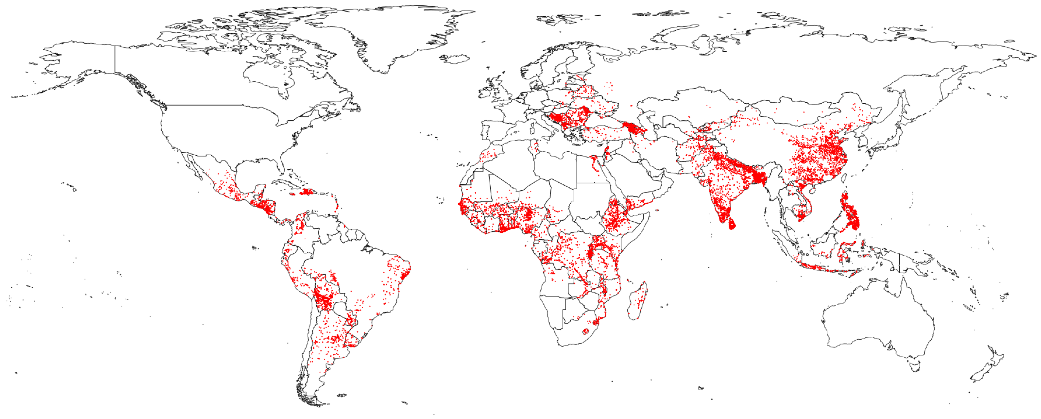
Despite these shifts in the policies of donor agencies, there is a gap in empirical studies examining the impacts of these policies on environmental outcomes. This research aims to illustrate an approach to overcoming this gap, as well as highlight many of the remaining methodological challenges. We specifically examine the impact of large-scale World Bank projects on vegetation and subsequent changes in carbon sequestration, leveraging a novel and publicly available data set of 61,243 World Bank project locations (see
Figure 1) from AidData in conjunction with long-term satellite data quantifying vegetative biomass and a number of spatially-referenced control variables (see
Table 1). We do not theorize on the explicit causal pathways for impact, instead seeking to identify evidence of where the World Bank has—or has not—met the goal of promoting neutral or positive environmental outcomes.
We find that while the overall impact of large scale World Bank projects on carbon sequestration appears to be positive, considerable temporal and spatial variation exists in these impacts. We illustrate the advantages and limitations of a geographically explicit approach to estimating the causal effects of development aid projects, and outline a number of topics for further research. Specifically, we discuss the need for hard assumptions of model independence in geographically explicit models to enable causal estimates, the concomitant limitations in interpretation this necessitates, and possible pathways forward to overcome this critical limitation. Finally, we introduce an enhanced publicly available data set of the global spatially-explicit distribution of World Bank activities encompassing projects initiated between 1995 and 2014.
2. Methods
Significant progress has been made in methods which integrate spatial data (i.e., satellite information on forest cover) to quantify the causal impact of interventions (i.e., projects aimed at the prevention of deforestation) [
7]. These nascent “top-down” approaches—or, approaches which primarily rely on remotely sensed or other already available data—offer great promise for cost-effective screening exercises to enable more targeted in-situ observational studies. These methods largely rely on propensity score and other matching-based methods to select “control” cases where no or limited intervention occurred, and match these with similar “treatment” cases at the sites of interventions [
8]. We build on these approaches, implementing a geographically explicit two-stage Propensity Score Matching estimation strategy. This is motivated by the context of this analysis: specifically, we hypothesize that the impact of World Bank projects is geographically heterogeneous—i.e., a project in the Sahara is unlikely to have the same impact as one in the Amazon. In this section, we detail one approach which enables researchers to measure impacts in a way that flexibly incorporates geographical heterogeneity, and in the discussion highlight many limitations and possible extensions.
2.1. Geographically Explicit Impacts
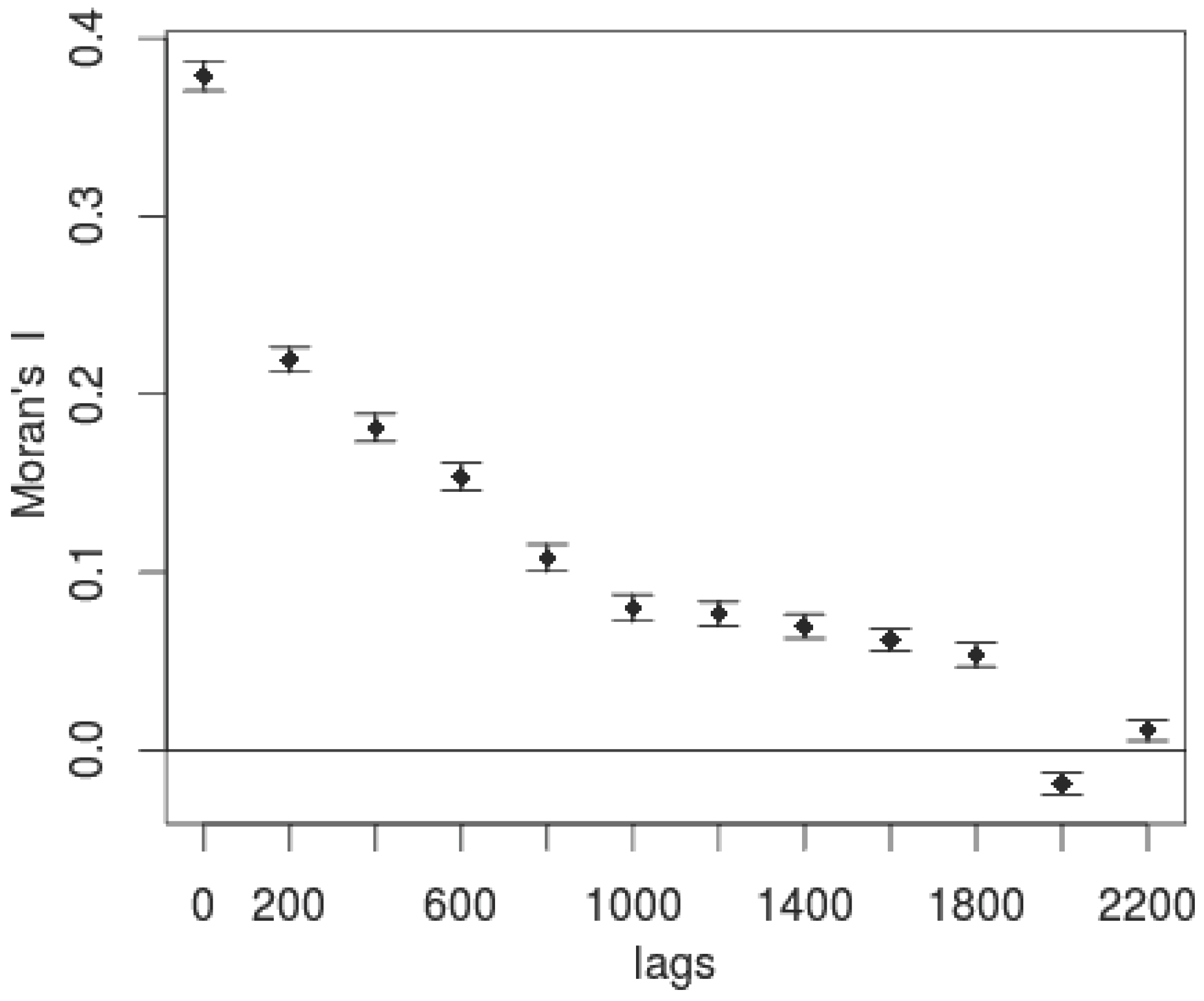
First, we subset the data to cover World Bank projects from 2000 to 2010 due to limitations of our ancillary information, resulting in a total of 41,306 World Bank project locations. From this, we remove data which do not have precise latitude and longitude information, leaving us with 19,940 locations. Second, the area of influence within which we anticipate each World Bank project could plausibly have an impact on deforestation is calculated by examining the historic spatial distance at which forest cover is spatially correlated. To parameterize this distance, we calculate a Moran’s I [
9] score at increasing distances—a metric that measures the degree of spatial autocorrelation for a given variable. We use this metric to estimate the distance at which spatial autocorrelation is no longer predominant for our outcome measure of forest cover, measured in 1999. We argue that this is a highly conservative estimate of the possible area of influence a project could have (i.e., we will tend to over-estimate the buffer size), as it represents the totality of historic spillovers up to the year 1999.
For each of 12 distance bins (between 0 and 2200 km, in increments of approximately 180 km), Moran’s I is calculated as follows:
where
h represents each spatial bin,
N the number of spatial units,
i and
j are indexes for each unit,
X is the variable of interest, and
represents the weights matrix. In this application, the weights matrix is specified according to the bin (
h) being analyzed.
Once calculated, the distance at which Moran’s I is equal to or less than 0.10 is identified, and used to parameterize a buffer around each project location. The project locations are then subdivided into six different groups based on project sectors—Health, Environment, Education, Industrial, Infrastructure, and Other. For each sector group, the respective locations are further subdivided into three equally-sized monetary bins of “low”, “medium”, and “high” based on dollars committed.
Finally, for the high dollar value group, a geographically explicit propensity score model is fit. This is conducted following a three-stage process which is repeated for every high dollar value World Bank project location, resulting in a model for each of the project locations. In the first stage, a high dollar value World Bank project location is selected, and all World Bank projects that fall within the distance threshold estimated according to the Moran’s I are selected as the relevant “subpopulation” for that point. All points within the subpopulation are defined as treated or untreated pending their monetary value—units of observation with a high dollar value (in the upper 33% for a given sector) are assigned as treated (1), while all projects in the low bin (in the lower 33% for a sector) are assigned an untreated value (0).
In the second stage, all points within the subpopulation are matched according to a propensity score matching routine. Variables matched on can be seen in
Table 1, with the goal of minimizing the difference between matched treated (areas with a large dollar value World Bank project) and untreated (areas with a small dollar value World Bank project) units along observed dimensions using a propensity matching approach. These dimensions include, for example, measures of proximity to roads, nighttime lights, and initial forest cover states. Matching along such dimensions seek to ensure that pairs have similar values in terms of observable sources of potential bias; i.e., two locations close to roads may be more likely to experience deforestation than two far from roads. By matching along observable dimensions, these routines hope to minimize the potential for omitted variable biases (i.e., unobserved variables), under the assumption that units similar along all observable dimensions are more likely to be similar along unobserved dimensions (extensive discussions of propensity score matching and its application can be found in [
10,
11]). The propensity scores are calculated following a logit model:
where
T is the treatment binary, and
are the estimated coefficients for each covariate,
.
The estimates from this equation are applied to each unit of observation within the subpopulation, and the differences between propensity scores across different units of observation are used to represent a univariate measure of similarity. For the set of high dollar value locations within the area of influence, the optimal set of matched untreated units (without replacement) are identified using a nearest-neighbor optimization [
12]. This results in a dataset in which each treated unit is matched with the single control unit most similar to it, with units that have no meaningful comparison dropped from the analysis (see
Table 2).
In the third stage, a linear regression relationship is estimated between the outcome measure (the average NDVI value in the years after project implementation), the treatment binary, and all available covariates (a traditional, ordinary least squares model is fit using QR decomposition to promote the computational feasibility of this approach, but the authors note that other modeling approaches (Spatial Autoregressive, Generalized Linear Models) may be more appropriate in some use cases). As contrasted to linear modeling efforts where the goal might be to improve model fit, here the primary goal is to ensure that the parameters estimated for the treatment binary (
θ) are accurate:
where
represents the level of forest cover within each zone
i,
θ represents the estimated impact of the treatment,
represents a fixed effect for each paired observation, and
represents a sector-specific fixed effect. Every unit of observation
n has a zone
i, defined as all locations which fall within the distance calculated using Moran’s I.
This process is repeated for every unit of observation in the high dollar value subset. In some cases, insufficient matches or eligible cases existed to approximate the impact for a region; these units were omitted from the analysis.
2.2. Estimating Carbon Sequestration
Because the outcome measure examined (NDVI) is only a proxy for carbon, an additional step of modeling must be conducted to translate changes in NDVI into changes in estimated relative tonnes of carbon sequestered. To accomplish this, we employ a fixed-effects approach to account for the geographically variable relationship between NDVI and carbon (a heterogeneous relationship largely driven by different floral regimes across the globe). This relies on two datasets: an estimate of global vegetative carbon stocks representing the year circa 2000 [
5], and ecofloristic zone information representing key geographic divisions of flora relevant for carbon [
6]. Using this information in conjunction with LTDR NDVI from 2000, a fixed effect model is fit:
where
represents a fixed effect for each of 60 ecofloristic zones. The ecofloristic zone that each World Bank project exists in is then identified and used in conjunction with the impacts estimated in the geographically explicit methodology outlined above to estimate the relative carbon sequestration attributable to a given World Bank project location (tonnes/ha).
3. Results
First, we use the Moran’s I measurements (Equation (
1)) to select a buffer radius to use in the estimation of each individual location. As
Figure 2 illustrates, the distance-decay function of NDVI in 1999 follows an expected pattern, with spatial autocorrelation dropping off as distances increase. We use this information to select a buffer radius of 800 km as our threshold (Moran’s I = 0.10). For each unit of analysis, we then draw a subpopulation of all locations which fall within the 800 km radius.
For each of these subpopulations, we match control and treatment cases on the basis of the propensity scores estimated in Equation (
2), following a nearest-neighbor matching strategy. A caliper of 0.25 is used to exclude poor matches, and after matching, if a sufficient total of matches does not exist (less than 30 total matches), the unit is excluded from analysis and we move to the next subpopulation.
After matching is conducted for each subpopulation, a regression is performed for that subpopulation following Equation (
3). This results in 8399 locations which have adequate matches for estimation, or 47% of all large-scale projects’ locations. For each of these models, we record all relevant information regarding standard errors and estimated coefficients. The impacts estimated for each of these locations (
θ and the sector-specific interaction term in Equation (
3)) are entered into the fixed-effect model derived following Equation (
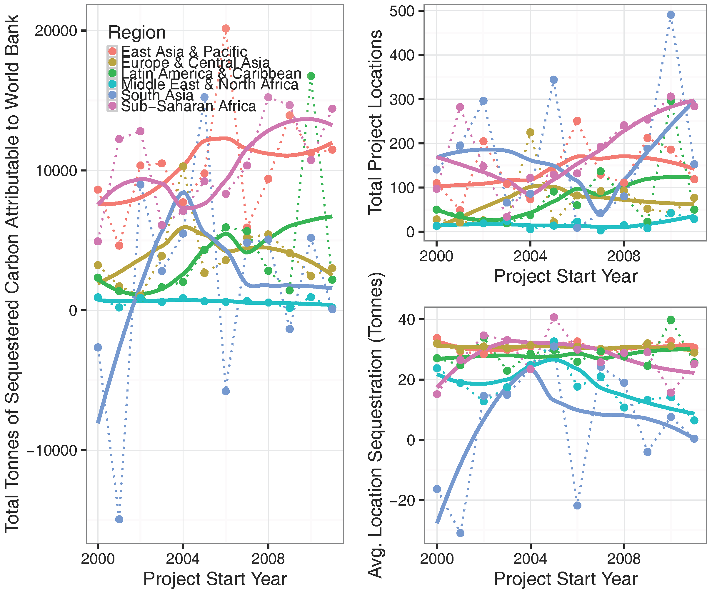
4). This provides a regionally-specific estimate of the tonnes of carbon sequestered attributable to a World Bank project (tonnes/ha). A regional- and temporal-disaggregation of the results across all estimated projects can be seen in
Figure 3. Individual estimates for projects—as well as estimated uncertainties—can be found in a dynamic online appendix (see [
13]).
4. Discussion and Conclusions
The approach outlined in this document highlights a number of interesting findings, but is constrained by significant methodological limitations. Of the key findings, we highlight the general improvement of World Bank projects over time, most notably in south Asia—a trend which could be reflective of functional environmental safeguards. However, we also highlight the significant geographic variation in this finding. For example, development projects in India almost universally had relatively negative impacts on sequestration, while those in the Philippines had relatively positive impacts. This is also evident on a region-by-region basis, as the negative trend line within the Middle East and North Africa highlights (see
Figure 3).
As shown in the online appendix, there is significant geographic variation—even across small areas—in the impact of World Bank projects on carbon sequestration. This variation is in-and-of-itself informative: for example, projects in southern Latin America tend to nearly universally outperform those located in Mexico; within Mexico, projects closer to Mexico City tend to have slightly better performance than those in the northern regions of the country. Considering that country-specific effects are not explicitly entered into the model, such country differences can lead to new types of questions regarding why projects are performing well within some areas in a region and poorly in others. Intra-country differences can lead to similar types of inquiry: why are some bright spots emerging in Mexico, despite the more negative outcomes observed in much of the country? Exploration of these questions from a "bottom up" in-situ perspective could allow for deeper insights into the causal mechanisms driving (or failing to drive) impacts on carbon sequestration; the methodology presented here can help to better target such efforts.
This approach has the benefit of contrasting World Bank locations to other locations at which it is known a World Bank project (albeit of a small magnitude) exists, and comparisons are conducted within projects that are at least known to be within the same sector. Contrasted to the "null case" comparison—where World Bank projects are contrasted to areas at which no World Bank projects existed—this approach allows an increased confidence that the processes and patterns being compared are similar in key ways. However, this choice has two key negative implications. First, the external validity of the study is questionable; because World Bank projects are not sited randomly, our findings may only hold for the set of projects analyzed here. For our particular application, this is an acceptable tradeoff, but this may not be the case in all contexts. Second, because our contrast group is known locations where World Bank projects exist, we may provide inaccurate absolute estimates if small-scale projects cause large impacts on carbon sequestration. There is limited evidence that this would be the case, but is a potential direction for future research.
By leveraging the geographic context in which projects exist, this approach has the potential to improve matches by providing pairs which are contextually similar—i.e., projects in dense forests are compared to other projects in dense forests; those near urban areas are contrasted to others near urban areas. Both of these attributes help to mitigate concerns over omitted variable biases, though they come with drawbacks (noted below). Lastly, by leveraging the geographically explicit approach detailed here, each location receives an estimated impact. Thus, the geographical subpopulations generated in this approach provide unique insights into trends that may vary over space.
Many opportunities exist to advance research which seeks to incorporate geographic data into models which causally identify impacts. First and foremost are the well known disadvantages to geographically weighted regression (GWR) approaches—namely, spatial correlation in estimated coefficients, bias in standard error terms [
14], and the necessity to define a weights matrix (i.e., in this piece, we use a Moran’s I based threshold to approximate a single distance threshold, but many alternative means for estimation of relevant thresholds exist). The approach selected to construct a weights matrix is of particular importance for causally-identified models, as one must ensure that the approach selected will not introduce potential bias into your estimates around
θ. Traditional approaches—i.e., co-kriging—which include information on covariates (or, even the treatment itself) can be susceptible to this problem under some circumstances, necessitating careful consideration. While we use Moran’s I to attempt to mitigate this concern, the univariate nature of Moran’s I is a double edged sword - by examining only spillover in NDVI before treatment was implemented, we prevent potential endogeneity in our threshold but omit potentially useful information on what the plausible range of World Bank project impacts in particular might be (instead only being able to estimate the cumulative historic impact on NDVI as a whole). There are additionally remaining concerns regarding the Stable Unit Treatment Value Assumption (SUTVA), as World Bank projects may experience spillover that is not adequately captured in the approach presented here. These factors limit the interpretation of the estimates calculated in this paper, specifically preventing insights into the significance of treatment impacts at any single project location. Ongoing research is examining potential solutions to this problem—for example, modifications to the techniques of Seemingly Unrelated Regression (SUR) or emergent causal machine learning approaches (see [
15]), but much of this research is currently nascent, and solutions appear to be extremely computationally intensive. Autoregressive approaches to model fitting may be valuable for mitigating concerns related to spatial spillover from World Bank projects, but relatively little literature has explored the pros or cons of such models in the context of causal inferential models (with a small number of notable exceptions, including [
16]).
A second limitation of this approach is in the matching strategy employed. We chose to contrast high-dollar value World Bank projects to low-dollar value World Bank projects, but outside of sectoral information have relatively little knowledge regarding the actual projects that were implemented at any given site. While we incorporate sectoral-specific fixed effects to ensure—to the degree possible—that we are comparing “apples to apples”, and further mitigate this problem by only selecting projects for which exact geographic information is available (thus omitting many broader, country-level initiatives that are rarely immediately associated with physical land change), the potential for bias due to poor comparison still exists. This is representative of a broader concern of any top-down approaches to impact evaluation, as there is frequently limited information on the characteristics of the project and relevant geographic contextual factors to include. Ongoing research into key characteristics of projects (i.e., beyond the number of dollars allocated and sectoral grouping, and including factors such as spatial correlation amongst covariates) seeks to mitigate these concerns, and provide increasingly better matches when top-down strategies are pursued.
A third limitation is in the available sources of data for these types of analyses. There are many different data products which seek to quantify vegetation—ranging from forest cover to vegetation density—and all come with many opportunities and drawbacks. Here, we selected NDVI due to the length of the satellite record; leveraging the NASA LTDR record, we are able to observe over thirty years of trends. However, NDVI is prone to issues such as saturation over dense regions, making it difficult to detect some important changes. Alternatives such as the Enhanced Vegetation Index—or, more recent high-resolution land cover products such as those produced by Hansen et al. [
17]—may be more appropriate for other case studies.
Despite these limitations, we believe this approach provides policymakers with a cost-effective approach to rapidly assess a very large portfolio of projects to identify “warning flags” or “bright spots”. We do not suggest that such analyses take the place of traditional impact evaluation strategies, but rather argue that top-down analyses such as these can help better direct resources for more rigorous in-situ assessments. Further, because we leverage satellite information which is regularly updated, such strategies could be applied not only to project evaluation, but also project monitoring.
Following this, we argue that sub-national data can be helpful in the identification of geographically heterogeneous impact effects. This piece highlights this by examining the impact of large-scale World Bank projects on carbon sequestration at a global scale, using a novel and publicly available data set of World Bank project locations. We find that while these projects appear to have an overall positive effect, significant temporal and geographic variation exists which would be masked if single aggregate estimates were examined. Finally, we argue for the importance of further research into methods to estimate geographically heterogeneous impacts effects.


