
An Economic Assessment of Local Farm Multi-Purpose Surface Water Retention Systems under Future Climate Uncertainty


Abstract
:1. Introduction
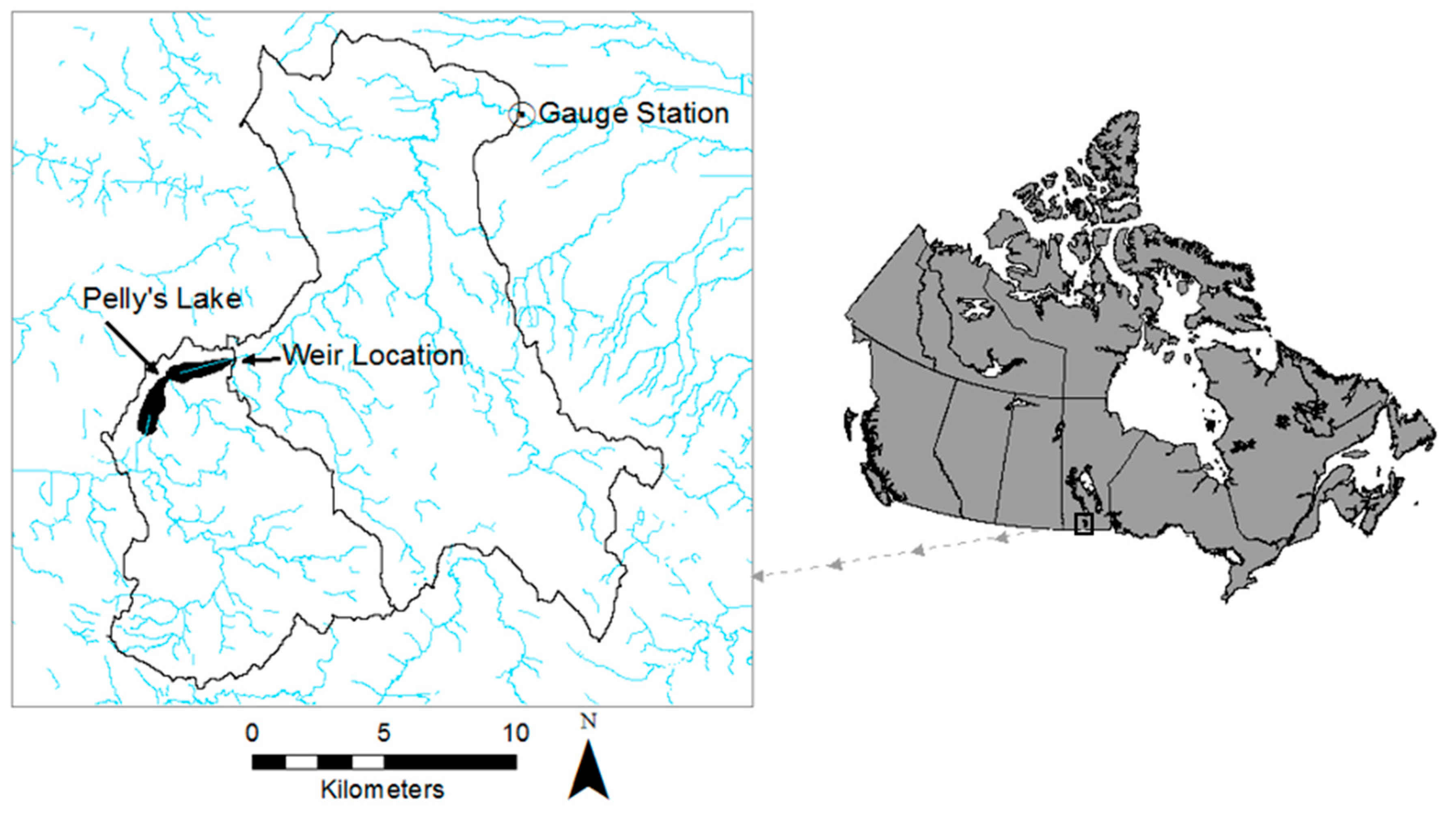
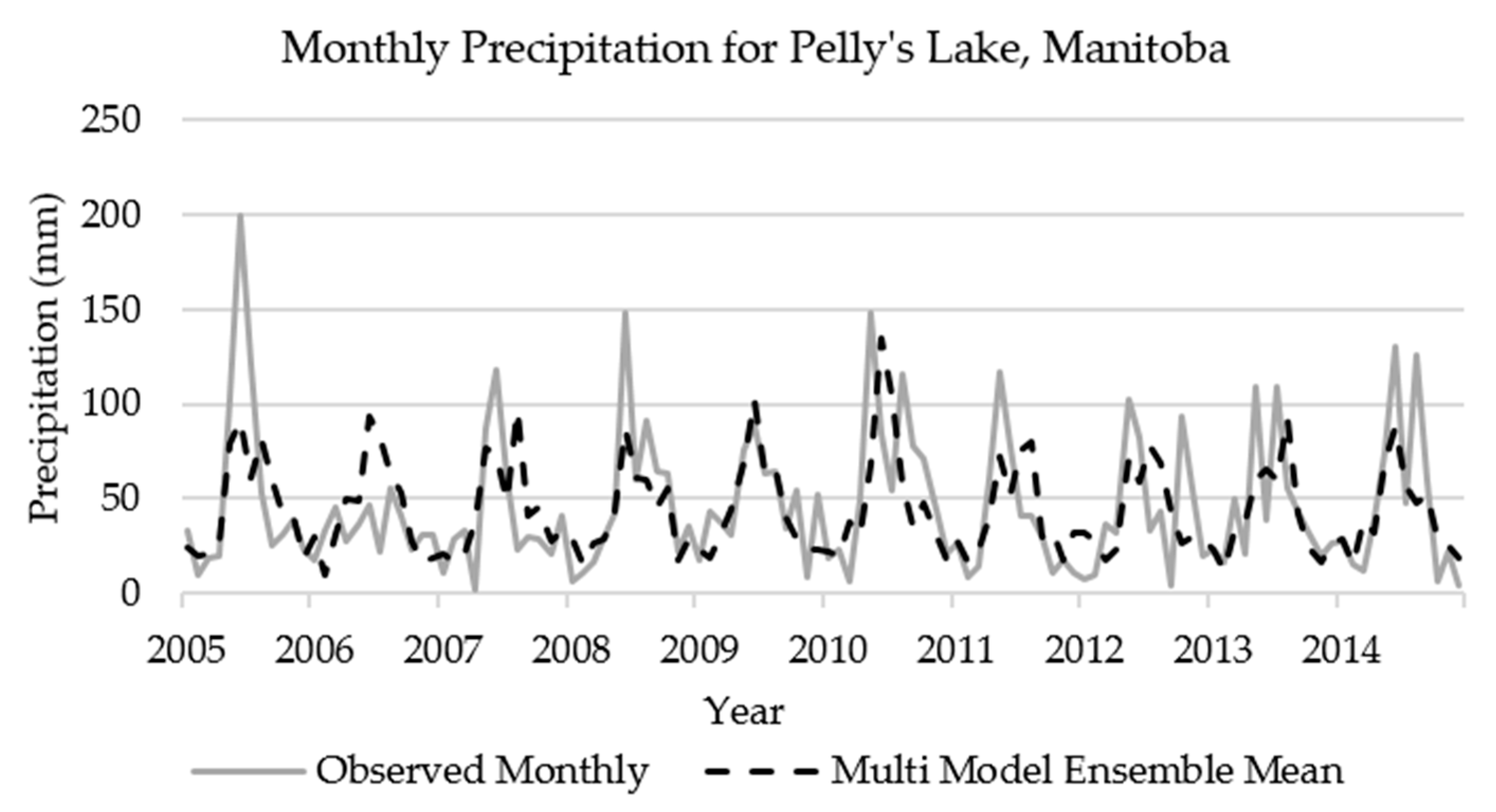
Study Site
2. Materials and Methods
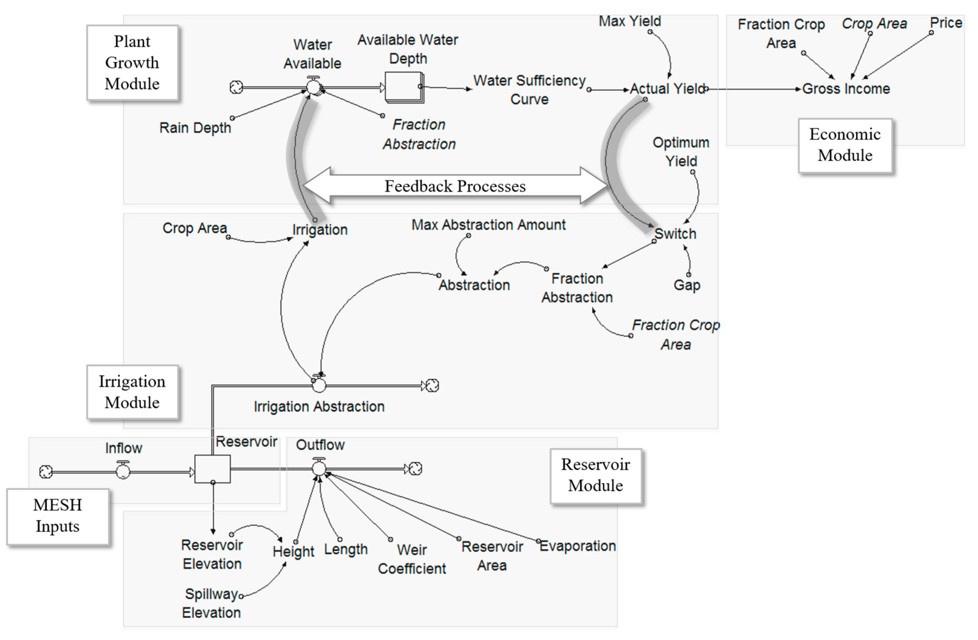
2.1. Modeling System
2.1.1. Hydrologic Model and Reservoir Module
2.1.2. Irrigation and Plant Growth Module
2.1.3. Economic Module
2.2. Climate Change
2.2.1. Delta Method
2.2.2. Uncertainty
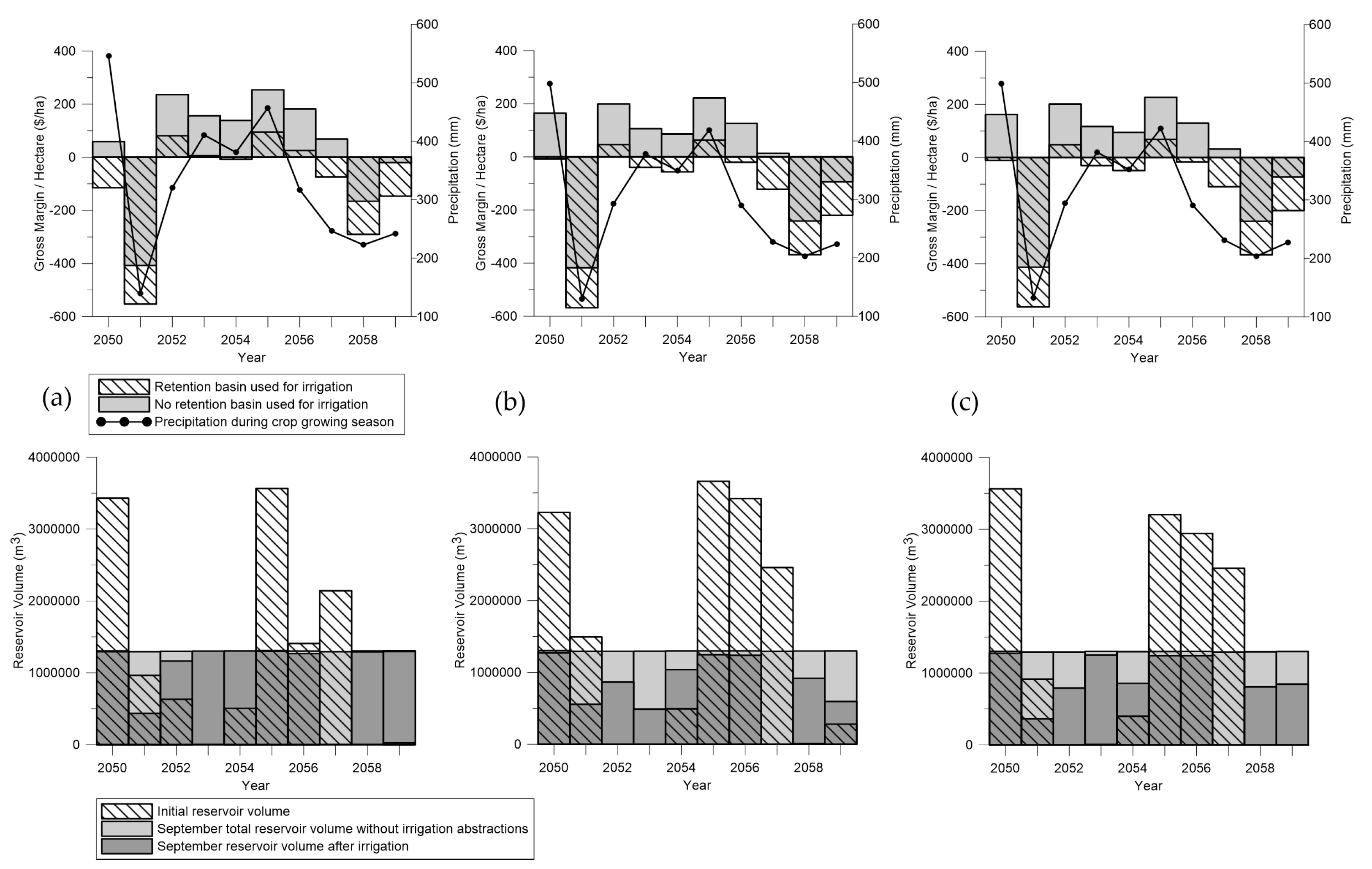
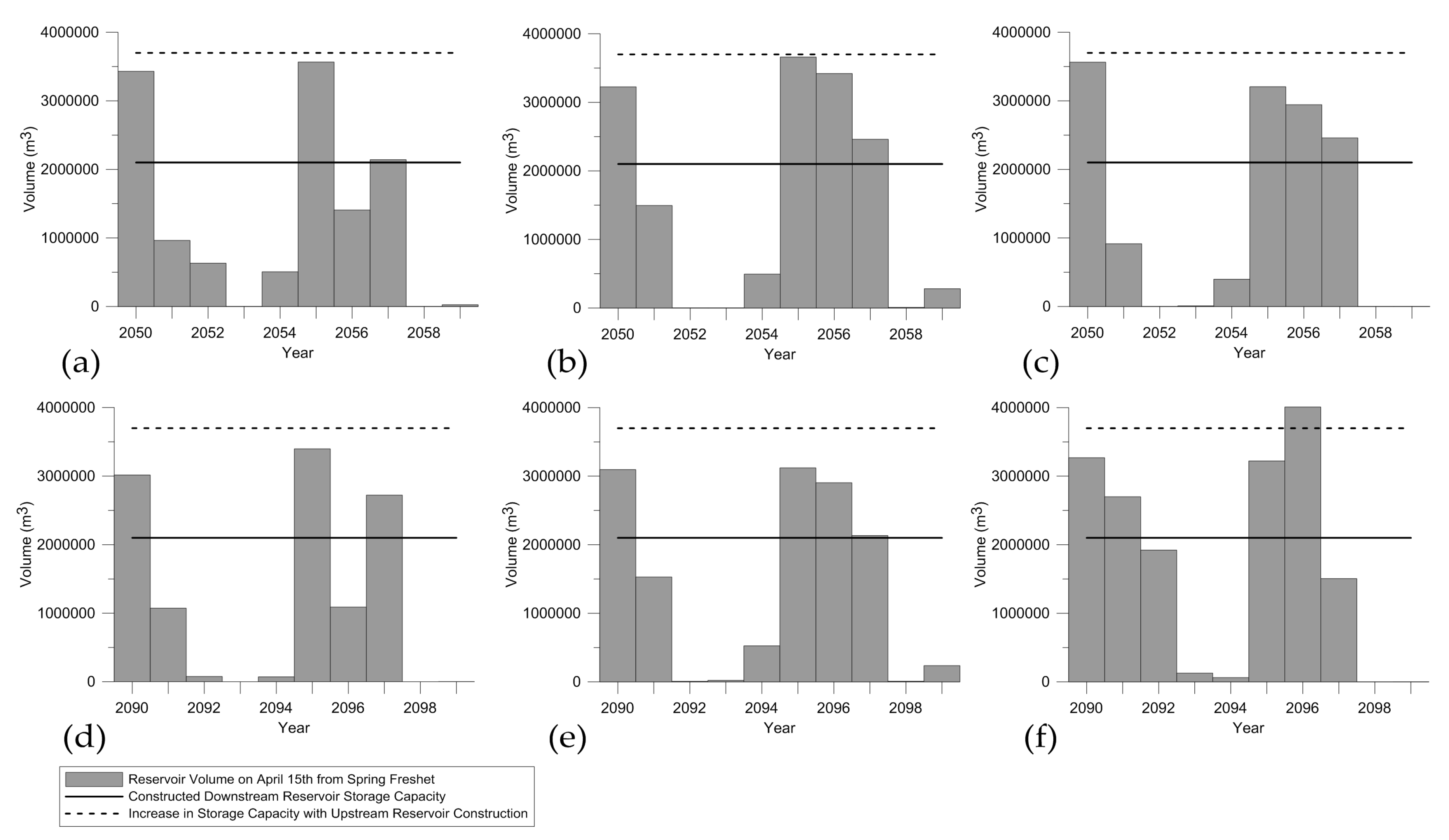
3. Results
4. Discussion
Future Directions
5. Conclusions
Acknowledgments
Author Contributions
Conflicts of Interest
References
- Warren, F.J.; Lemmon, D.S. (Eds.) Synthesis; in Canada in a Changing Climate: Sector Perspectives on Impacts and Adaptation; Government of Canada: Ottawa, ON, Canada, 2014. Available online: http://www.nrcan.gc.ca/environment/resources/publications/impacts-adaptation/reports/assessments/2014/16309 (accessed on 3 January 2016).
- Vincent, L.A.; Wang, X.L.; Milewska, E.J.; Wan, H.; Yang, F.; Swail, V. A second generation of homogenized Canadian monthly surface air temperature for climate trend analysis. J. Geophys. Res. Atmos. 2012, 117, 1–13. [Google Scholar] [CrossRef]
- Venema, H.D.; Oborne, B.; Neudoerffer, C. The Manitoba Challenge: Linking Water and Land Management for Climate Adaptation; International Institute for Sustainable Development: Winnipeg, MB, Canada, 2010. [Google Scholar]
- Bonsal, B.R.; Wheaton, E.E.; Chipanshi, A.C.; Lin, C.; Sauchyn, D.J.; Wen, L. Drought research in Canada: A review. Atmos. Ocean 2011, 49, 303–319. [Google Scholar] [CrossRef]
- Intergovernmental Panel on Climate Change (IPCC). Climate Change 2007: Synthesis Report. Contribution of Working Groups I, II, and III to the Fourth Assessment Report of the Intergovernmental Panel on Climate Change; Core Writing Team, Pachauri, R., Reisinger, A., Eds.; IPCC: Geneva, Switzerland, 2007. [Google Scholar]
- Hearne, R.R. Evolving water management institutions in the Red River Basin. Environ. Manag. 2007, 40, 842–852. [Google Scholar] [CrossRef] [PubMed]
- Wheaton, E.; Kulshreshtha, S.; Wittrock, V.; Koshida, G. Dry times: Hard lessons from the Canadian drought of 2001 and 2002. Can. Geogr. 2008, 52, 241–262. [Google Scholar] [CrossRef]
- Wall, E.; Smit, B. Climate Change Adaptation in Light of Sustainable Agriculture. J. Sustain. Agric. 2005, 27, 113–123. [Google Scholar] [CrossRef]
- Pittman, J.; Wittrock, V.; Kulshreshtha, S.; Wheaton, E. Vulnerability to climate change in rural Saskatchewan: Case study of the Rural Municipality of Rudy No. 284. J. Rural Stud. 2011, 27, 83–94. [Google Scholar] [CrossRef]
- Belcher, K. Agroecosystem Sustainability: An Integrated Modeling Approach. Ph.D. Thesis, University of Saskatchewan, Saskatoon, SK, Canada, 1999. [Google Scholar]
- Samarawickrema, A.; Kulshreshtha, S. Value of irrigation water for drought proofing in the South Saskatchewan River Basin (Alberta). Can. Water Resour. J. 2008, 33, 273–282. [Google Scholar] [CrossRef]
- Bower, S.S. Watersheds: Conceptualizing Manitoba’s Drained Landscape, 1985–1950. Environ. Hist. Durh. N. C. 2007, 12, 796–819. [Google Scholar] [CrossRef]
- La Salle Redboine Conservation District. La Salle River Watershed: State of the Watershed Report, 2007. pp. 1–296. Available online: https://www.gov.mb.ca/waterstewardship/iwmp/whitemud/documentation/summary_lasalle.pdf (accessed on 23 November 2015).
- Government of Manitoba. Surface Water Management Strategy; Government of Manitoba: Winnipeg, MB, Canada, 2014. Available online: http://gov.mb.ca/waterstewardship/questionnaires/surface_water_management/pdf/surface_water_strategy_final.pdf (accessed on 1 October 2015).
- Manitoba Government. Conservation and Water Stewardship. Available online: http://mli2.gov.mb.ca/ (accessed on 1 September 2014).
- Pavelic, P.; Srisuk, K.; Saraphirom, P.; Nadee, S.; Pholkern, K.; Chusanathas, S.; Munyou, S.; Tangsutthinon, T.; Intarasut, T.; Smakhtin, V. Balancing-out floods and droughts: Opportunities to utilize floodwater harvesting and groundwater storage for agricultural development in Thailand. J. Hydrol. 2012, 470–471, 55–64. [Google Scholar] [CrossRef]
- Grosshans, R.E.; Gass, P.; Dohan, R.; Roy, D.; Venema, H.D.; McCandless, M. Cattail Harvesting for Carbon Offsets and Nutrient Capture: A Lake Friendly Greenhouse Gas Project; International Institute for Sustaianble Development: Winnipeg, MB, Canada, 2012; Available online: http://www.iisd.org/library/cattails-harvesting-carbon-offsets-and-nutrient-capture-lake-friendly-greenhouse-gas-project (accessed on 3 November 2015).
- Government of Canada. Agriculture and Agri-Food Canada Positive Effects of Small Dams and Reservoirs: Water Quality and Quantity Findings from a Prairie Watershed; WEBS Fact Sheet #7; Government of Canada: Ottawa, ON, Canada, 2012. Available online: http://www.agr.gc.ca/eng/?id=1351881784186 (accessed on 24 April 2016).
- Arnold, J.G.; Stockle, C.O. Simulation of Supplemental Irrigation from On-Farm Ponds. J. Irrig. Drain. Eng. 1991, 117, 408–424. [Google Scholar] [CrossRef]
- Berry, P. An economic Assessment of On-Farm Surface Water Retention Systems. Ph.D. Thesis, University of Saskatchewan, Saskatoon, SK, Canada, 2016. [Google Scholar]
- Tiessen, K.H.D.; Elliott, J.A.; Stainton, M.; Yarotski, J.; Flaten, D.N.; Lobb, D.A. The effectiveness of small-scale headwater storage dams and reservoirs on stream water quality and quantity in the Canadian Prairies. J. Soil Water Conserv. 2011, 66, 158–171. [Google Scholar] [CrossRef]
- Sharpley, A.; Smith, S.J.; Zollweg, J.A.; Coleman, G.A. Gully treatment and water quality in the Southern Plains. J. Soil Water Conserv. 1996, 51, 498–503. [Google Scholar]
- Kovacic, D.A.; Twait, R.M.; Wallace, M.P.; Bowling, J.M. Use of created wetlands to improve water quality in the Midwest-Lake Bloomington case study. Ecol. Eng. 2006, 28, 258–270. [Google Scholar] [CrossRef]
- Salvia-Castellvi, M.; Dohet, A.; Vander Borght, P.; Hoffmann, L. Control of the eutrophication of the reservoir of Esch-sur-Sûre (Luxembourg): Evaluation of the phosphorus removal by predams. Hydrobiologia 2001, 459, 61–71. [Google Scholar] [CrossRef]
- Avilés, A.; Niell, F.X. The control of a small dam in nutrient inputs to a hypertrophic estuary in a Mediterranean climate. Water Air Soil Pollut. 2007, 180, 97–108. [Google Scholar] [CrossRef]
- Uusi-Kämppä, J.; Braskerud, B.; Jansson, H.; Syversen, N.; Uusitalo, R. Buffer zones and constructed wetlands as filters for agricultural phosphorus. J. Environ. Qual. 2000, 29, 151–158. [Google Scholar] [CrossRef]
- Chrétien, F.; Gagnon, P.; Thériault, G.; Guillou, M. Performance analysis of a wet-retention pond in a small agricultural catchment. J. Environ. Eng. 2016, 142, 4016005. [Google Scholar] [CrossRef]
- Manitoba Liquor and Lotteries Corporation. Environmental Innovation. Available online: http://www.mbll.ca/content/environmental-innovation (accessed on 12 December 2016).
- Brander, L.; Brouwer, R.; Wagtendonk, A. Economic valuation of regulating services provided by wetlands in agricultural landscapes: A meta-analysis. Ecol. Eng. 2013, 56, 89–96. [Google Scholar] [CrossRef]
- Olewiler, N. The Value of Natural Capital in Settled Areas of Canada; Ducks Unlmited and the Nature Conservancy of Canada: Stonewall, MB, Canada, 2004; Available online: http://www.cmnbc.ca/sites/default/files/natural%2520capital_0.pdf (accessed on 5 May 2016).
- Wilson, S. Ontario’s Wealth, Canada’s Future: Appreciating the Value of the Greenbelt’s Eco-Services; David Suzuki Foundation: Vancouver, BC, Canada, 2008; Available online: http://www.davidsuzuki.org/publications/downloads/2008/DSF-Greenbelt-web.pdf (accessed on 5 May 2016).
- Sohngen, B.; King, K.W.; Howard, G.; Newton, J.; Forster, D.L. Nutrient prices and concentrations in Midwestern agricultural watersheds. Ecol. Econ. 2015, 112, 141–149. [Google Scholar] [CrossRef]
- Collins, A.R.; Gillies, N. Constructed Wetland Treatment of Nitrates: Removal Effectiveness and Cost Efficiency. J. Am. Water Resour. Assoc. 2014, 50, 898–908. [Google Scholar] [CrossRef]
- Grosshans, R.; Grieger, L.; Ackerman, J.; Gauthier, S.; Swystun, K.; Gass, P.; Roy, D. Cattail Biomass in a Watershed-Based Bioeconomy: Commercial-Scale Harvesting and Processing for Nutrient Capture, Biocarbon and High-Value Bioproducts; International Institute for Sustainable Development: Winnipeg, MB, Canada, 2014; Available online: http://www.iisd.org/sites/default/files/publications/cattail-biomass-watershed-based-bioeconomy-commerical-scale-harvesting.pdf (accessed on 17 January 2015).
- Dion, J.; McCandless, M. Cost-Benefit Analysis of Three Proposed Distributed Water Storage Options for Manitoba; International Institute for Sustainable Development: Winnipeg, MB, Canada, 2013; Available online: http://www.iisd.org/pdf/2014/mb_water_storage_options.pdf (accessed 23 December 2014).
- McMinn, W.R.; Yang, Q.; Scholz, M. Classification and assessment of water bodies as adaptive structural measures for flood risk management planning. J. Environ. Manag. 2010, 91, 1855–1863. [Google Scholar] [CrossRef] [PubMed]
- Government of Canada. Government of Canada; Statistics Canada; Government of Canada: Ottawa, ON, Canada, 2015; pp. 2–6. Available online: www.statcan.gc.ca/eng/start (accessed on 15 September 2015).
- La Salle Redboine Conservation District. Pelly’s Lake Backflood Project; La Salle Redboine Conservation District: Holland, MB, Canada, 2013; pp. 1–2. Available online: www.lasalleredboine.com/pellys-lake-backflood-project (accessed on 28 August 2015).
- La Salle Redboine Conservation District. About. Available online: http://www.lasalleredboine.com/ (accessed on 24 November 2015).
- Armstrong, R.N.; Pomeroy, J.W.; Martz, L.W. Estimating evaporation in a prairie landscape under drought conditions. Can. Water Resour. J. 2010, 35, 173–186. [Google Scholar] [CrossRef]
- Pomeroy, J.; Fang, X.; Williams, B. Modelling Snow Water Conservation on the Canadian Prairies; University of Saskatchewan: Saskatoon, SK, Canada, 2011; Available online: http://www.usask.ca/hydrology/reports/CHRpt11_Prairie-Shelterbelt-Study_Apr11.pdf (accessed on 5 February 2015).
- Costanza, R.; Duplisea, D.; Kautsky, U. Ecological Modelling on modelling ecological and economic systems with STELLA. Ecol. Model. 1998, 110, 1–4. [Google Scholar]
- Pietroniro, A.; Fortin, V.; Kouwen, N.; Neal, C.; Turcotte, R.; Davison, B.; Verseghy, D.; Soulis, E.D.; Caldwell, R.; Evora, N.; et al. Development of the MESH modelling system for hydrological ensemble forecasting of the Laurentian Great Lakes at the regional scale. Hydrol. Earth Syst. Sci. 2007, 11, 1279–1294. [Google Scholar] [CrossRef]
- Verseghy, D.L. CLASS—A Canadian Land Surface Scheme for GCMS. I. Soil Model. Int. J. Climatol. 1991, 11, 111–133. [Google Scholar] [CrossRef]
- University of Saskatchewan. MEC—Surface and Hydrology (MESH). Available online: http://www.usask.ca/ip3/models1/mesh.htm (accessed on 15 October 2015).
- Verseghy, D.L.; McFarlane, N.A.; Lazare, M. CLASS—A Canadian Land Surface Scheme for GCMS. II. Vegetation Model and Coupled Runs. Int. J. Climatol. 1993, 13, 347–370. [Google Scholar] [CrossRef]
- Mahfouf, J.-F.; Brasnett, B.; Gagnon, S. A Canadian Precipitation Analysis (CaPA) project: Description and preliminary results. Atmos. Ocean 2007, 45, 1–17. [Google Scholar] [CrossRef]
- Côté, J.; Desmarais, J.-G.; Gravel, S.; Methot, A.; Patoine, A.; Roch, M.; Staniforth, A. The operational CMC—MRB Global Environmental Multiscale (GEM) Model. Part II: Results. Mon. Weather Rev. 1998, 126, 1397–1418. [Google Scholar] [CrossRef]
- Kouwen, N.; ASCE, M.; Soulis, E.D.; Pietroniro, A.; Donald, J.; Harrington, R.A. Grouped Response Units for Distributed Hydrologic Modeling. J. Water Resour. Plan. Manag. 1993, 119, 289–305. [Google Scholar] [CrossRef]
- Government of Manitoba. Guidelines for Estimating Crop Production Costs 2015; Government of Manitoba: Winnipeg, MB, Canada, 2015. Available online: https://www.gov.mb.ca/agriculture/business-and-economics/financial-management/cost-of-production.html (accessed on 15 January 2015).
- Statistics Canada. The Financial Picture of Farms in Canada. Available online: http://www.statcan.gc.ca/ca-ra2006/articles/finpicture-portrait-eng.htm (accessed on 25 January 2017).
- Waelti, C.; Spuhler, D. Retention Basin. Available online: http://www.sswm.info/content/retention-basin (accessed on 14 August 2014).
- Grinder, B. Alberta’s Irrigation Infrastructure; Government of Alberta: Lethbridge, AB, Canada, 2000. Available online: http://www1.agric.gov.ab.ca/$department/deptdocs.nsf/all/irr7197 (accessed on 3 March 2015).
- Government of Manitoba. Personal communication, 2015.
- Government of Manitoba. Manitoba Land Initiative: Core Maps—Data Warehouse; Government of Manitoba: Winnipeg, MB, Canada. Available online: http://mli2.gov.mb.ca/mli_data/index.html (accessed on 23 September 2014).
- Government of Canada. Historical Climate Data. Available online: http://climate.weather.gc.ca/ (accessed on 15 February 2015).
- Belcher, K.W.; Boehm, M.M.; Fulton, M.E. Agroecosystem sustainability: A system simulation model approach. Agric. Syst. 2004, 79, 225–241. [Google Scholar] [CrossRef]
- Werner, A.T. BCSD Downscaled Transient Climate Projections for Eight Select GCMs over British Columbia, Canada; Pacific Climate Impacts Consortium, University of Victoria: Victoria, BC, Canada, 2011; Available online: https://pdfs.semanticscholar.org/5dc0/a283b244d177e30c12e1d48d8a227f3720f9.pdf (accessed on 4 January 2016).
- Pacific Climate Impacts Consortium Statistically Downscaled Climate Scenarios. Available online: https://www.pacificclimate.org/data/statistically-downscaled-climate-scenarios (accessed on 1 July 2016).
- Randall, D.A.; Wood, R.A.; Bony, S.; Colman, R.; Fichefet, T.; Fyfe, J.; Kattsov, V.; Pitman, A.; Shukla, J.; Srinivasan, J.; et al. Climate Models and Their Evaluation. In Climate Change 2007: The Physical Science Basis. Contribution of Working Group 1 to the Fourth Assessment Report of the Intergovernmental Panel on Climate Change; Soloman, S., Qin, D., Manning, M., Chen, Z., Marquis, M., Averyt, K.B., Tignor, M., Miller, H.L., Eds.; Cambridge University Press: Cambridge, UK; New York, NY, USA, 2007; p. 996. [Google Scholar]
- Schnorbus, M.; Werner, A.; Bennett, K. Impacts of climate change in three hydrologic regimes in British Columbia, Canada. Hydrol. Process. 2014, 28, 1170–1189. [Google Scholar] [CrossRef]
- Hamlet, A.F.; Salathé, E.P.; Carrasco, P. Statistical Downscaling Techniques for Global Climate Model Simulations of Temperature and Precipitation with Application to Water Resources Planning Studies; Chapter 4 in Final Report for the Columbia Basin Climate Change Scenarios Project; Climate Impacts Group, Center for Science in the Earth System, Joint Institute for the Study of the Atmosphere and Ocean, University of Washington: WA, USA, 2010; Available online: https://cig.uw.edu/publications/statistical-downscaling-techniques-for-global-climate-model-simulations-of-temperature-and-precipitation-with-application-to-water-resources-planning-studies/ (accessed on 27 December 2015).
- Werner, A.T.; Cannon, A.J. Hydrologic extremes—An intercomparison of multiple gridded statistical downscaling methods. Hydrol. Earth Syst. Sci. 2016, 20, 1483–1508. [Google Scholar] [CrossRef]
- Shrestha, R.; Schnorbus, M.A.; Werner, A.T.; Zwiers, F.W. Evaluating Hydroclimatic Change Signals from Statistically and Dynamically Downscaled GCMs and Hydrologic Models. J. Hydrometeorol. 2014, 15, 844–860. [Google Scholar] [CrossRef]
- Barrow, E. Climate Change Scenarios. In The Availability, Characteristics and Use of Climate Change Scenarios; Prairie Adaptation Research Collaborative: Regina, SK, Canada, 2001; Available online: http://www.parc.ca/pdf/conference_proceedings/jan_01_barrow1.pdf (accessed on 1 February 2017).
- Diaz-Nieto, J.; Wilby, R.L. A comparison of statistical downscaling and climate change factor methods: Impacts on low flows in the River Thames, United Kingdom. Clim. Chang. 2005, 69, 245–268. [Google Scholar] [CrossRef]
- Graham, L.P.; Andreáasson, J.; Carlsson, B. Assessing climate change impacts on hydrology from an ensemble of regional climate models, model scales and linking methods—A case study on the Lule River basin. Clim. Chang. 2007, 81, 293–307. [Google Scholar] [CrossRef]
- Chen, J.; Brissette, F.P.; Leconte, R. Uncertainty of downscaling method in quantifying the impact of climate change on hydrology. J. Hydrol. 2011, 401, 190–202. [Google Scholar] [CrossRef]
- Trzaska, S.; Schnarr, E. A Review of Downscaling Methods for Climate Change Projections; Tetra Tech ARD: Burlington, VT, USA, 2014. [Google Scholar]
- Intergovernmental Panel on Climate Change—Task Group on Data and Scenario Support for Impact and Climate Analysis (IPCC-TGICA). General Guidelines on the Use of Scenario Data for Climate Impact and Adaptation Assessment; Intergovernmental Panel on Climate Change: Geneva, Switzerland, 2007; Volume 2. Available online: http://www.ipcc-data.org/guidelines/TGICA_guidance_sdciaa_v2_final.pdf (accessed on 16 January 2016).
- Charron, I. A Guidebook on Climate Scenarios: Using Climate Information to Guide Adaptation Research and Decisions; Ouranos: Montreal, QC, Canada, 2014; Available online: https://www.ouranos.ca/publication-scientifique/GuideCharron2014_EN.pdf (accessed on 5 January 2016).
- Nyirfa, W.; Harron, B. Assessment of Climate Change on the Agricultural Resources of the Canadian Prairies; Prairie Adaptation Research Collaborative: Regina, SK, Canada, 2001; Available online: http://www.parc.ca/pdf/research_publications/agriculture4.pdf (accessed on 13 February 2016).
- Sauchyn, D.J.; Barrow, E.M.; Hopkinson, R.F.; Leavitt, P.R. Aridity on the Canadian Plains. Géogr. Phys. Quat. 2002, 56, 247–259. [Google Scholar] [CrossRef]
- Bourne, A.; Armstrong, N.; Jones, G. A Preliminary Estimate of Total Nitrogen and Total Phosphorus Loading to Streams in Manitoba, Canada; Government of Manitoba: Winnipeg, MB, Canada, 2002. Available online: http://www.gov.mb.ca/sd/eal/registries/4864wpgww/mc_nitrophosload.pdf (accessed 10 March 2016).
- Lake Winnipeg Stewardship Board. Reducing Nutrient Loading to Lake Winnipeg and Its Watershed: Our Collective Responsibility and Commitment to Action; Government of Manitoba: Winnipeg, MB, Canada, 2006. Available online: https://www.gov.mb.ca/waterstewardship/water_quality/lake_winnipeg/lwsb2007-12_final_rpt.pdf (accessed on 5 April 2016).


| Parameters/Units | Inputs and Equations with Descriptions | |
|---|---|---|
| Reservoir Module | ||
| Inflow (m3/day) | Input graphically using output data from the MESH hydrologic model on a daily time step. | |
| Reservoir (m3) | Initial reservoir volume calculated based on cumulative output from the MESH hydrologic model from 1 January–14 April. | |
| Outflow (m3/day) | =(3 × Weir_Coefficient × Length × Height1.5 × 86,400) − (Evaporation × Reservoir_Area) | |
| The established engineering equation for discharge over a rectangular weir was multiplied by 86,400 to convert from m3/s to m3/day. Evaporation over the reservoir area was subtracted from the discharge equation [54]. | ||
| Weir Coefficient (dimensionless) | =0.6, An established engineering value was used. | |
| Length (m) | =12, Spillway length was taken from the engineering drawings for the Pelly’s Lake weir. | |
| Height (m) | =IF (Reservoir Elevation − Spillway Elevation) > 0 THEN (Reservoir Elevation − Spillway Elevation) ELSE 0, An established engineering equation. | |
| Reservoir Elevation (m) | =9 × 10⁻⁷ × Reservoir + 378.23 | |
| This equation was determined from the engineering storage rating curve for the Pelly’s Lake weir. | ||
| Spillway Elevation (m) | =379.1, This value was provided on the engineering drawings for the Pelly’s Lake weir. | |
| Evaporation (m3/day) | =0.00182 (April) =0.00422 (May) =0.00460 (June) | =0.00454 (July) =0.00469 (August) =0.00346 (September) |
| Mean monthly evaporation values from 1981–2010 were converted to daily values at Brandon, MB [54]. These values were used due to insufficient data available to calculate evaporation at the study site. | ||
| Reservoir Area (m2) | =85,867,480, calculated in ArcGIS. | |
| Irrigation Module | ||
| Irrigation Abstraction (m3/day) | =Abstraction[Canola] + Abstraction[Wheat] + Abstraction[Barley] + Abstraction[Alfalfa], This variable calculated the total water abstraction volume abstracted from the reservoir. | |
| Abstraction [Crop] | =Max Abstraction Amount × Fraction Abstraction This equation calculated irrigation withdrawal volumes for each crop. | |
| Max Abstraction Amount (m3) | =15,000, this amount was calibrated to allow the reservoir to drain at a rate to provide sufficient water for irrigation for the entire growing season. | |
| Fraction Abstraction [Crop](dimensionless) | =IF ((Switch[Canola] + Switch[Wheat] + Switch[Barley] + Switch[Alfalfa]) > 0) THEN(Switch[Crop] × Fraction_Crop_Area[Crop]/(Switch[Canola] × Fraction_Crop_Area[Canola] + Switch[Wheat] × Fraction_Crop_Area[Wheat] + Switch[Barley] × Fraction_Crop_Area[Barley] + Switch[Alfalfa] × Fraction_Crop_Area[Alfalfa])) ELSE (0) | |
| When water requirements were not being met by a specific crop, this algorithm directed water withdrawals to the crop requiring irrigation. It also ensured water was not applied unless required to optimize crop growth. | ||
| Fraction Crop Area | =0.46 (Canola) =0.38 (Wheat) | =0.11 (Alfalfa) =0.05 (Barley) |
| Historical patterns of crop production in Manitoba were used to determine the fraction of total crop area each crop comprised [37,55]. | ||
| Switch[Crop] | =IF (Actual Yield < Gap × Optimum Yield AND TIME > 30 THEN 1 ELSE 0 | |
| Irrigation was triggered for a specific crop if the crop’s actual yield fell below 80% of optimum yield on day 30 (15 May). | ||
| Gap | =0.8, Irrigation application occurred when available water only allowed for 80% or less of optimum yield growth. Yield reductions due to water stress occur when available water falls below 60% of optimum plant requirements. The threshold of 80% ensured there was always sufficient water available to the plant [53]. | |
| Irrigation (mm/day) | =(Irrigation Abstraction/Crop Area) × 1000 | |
| This equation served to convert irrigation from a volume to a depth. | ||
| Crop Area (m2) | =66,976,634, This was calculated in ArcGIS using data on land use downloaded from the Manitoba Land Initiative [55]. | |
| Plant Growth Module | ||
| Rain Depth (mm/day) | Input graphically using values from Environment and Climate Change Canada for Holland, MB [56]. | |
| Water Available [Crop] (mm/day) | =Rain Depth + Irrigation × Fraction Abstraction | |
| Daily water available for crop growth [57]. | ||
| Available Water Depth [Crop] (mm) | Initial value set at 0. Snowmelt would contribute to initial spring soil moisture, however for the purposes of the model soil moisture was assumed to be recharged solely from precipitation and/or irrigation water. | |
| Water Sufficiency Curve [Crop] | These curves were input graphically and represented the unique optimal water requirements of each crop. They allowed for crop yield to be calculated based on water availability [57]. | |
| Max Yield [Crop](tonnes/m2) | = 0.000224124 (Canola) = 0.000336063 (Wheat) | =0.000376588 (Barley) =0.000672126 (Alfalfa) |
| Max yield values were held constant for all simulations [50]. | ||
| Actual Yield [Crop] (tonnes/hectare) | =Max Yield × Water Sufficiency Curve × 10,000 | |
| Crop yield was calculated based on water availability. Each crop’s water sufficiency curve provided a proportion of maximum growth based on water availability. This proportion was multiplied by max yield and 10,000 to convert from m2 to hectares. | ||
| Optimum Yield [Crop] | For each crop, values were input graphically. The variable represented the maximum yield of each crop over time when its water requirements were being met. Values were constant for all simulations. | |
| Economic Module | ||
| Gross Income [Crop] ($) | =Actual Yield × Price × Crop Area × Fraction Crop Area/10,000 Calculated landscape level gross income. | |
| Price [Crop] ($/tonne) | =418.87 (Canola) =238.83 (Wheat) | =173.23 (Barley) =132.28 (Alfalfa) |
| Crop prices were not available for years before 2015. Thus, 2015 crop prices were used in all simulations [50]. | ||
| RCP | Description |
|---|---|
| RCP2.6 | Radiative forcing will peak at approximately 3 W/m2 before 2100 and then levels will decline. |
| RCP4.5 | Radiative forcing will stabilize at 4.5 W/m2 after 2100. |
| RCP6 | Radiative forcing will stabilize at 6 W/m2 after 2100. |
| RCP8.5 | Radiative forcing will rise resulting in 8.5 W/m2 in 2100. |
| Modeling Center | Institute ID | Model Name |
|---|---|---|
| Canadian Centre for Climate Modeling and Analysis | CCCMA | CanESM2 |
| Meteorological Office Hadley Centre | MOHC | HadGEM2-ES |
| Max Planck Institute for Meteorology | MPI-M | MPI-ESM-LR |
| NOAA Geophysical Fluid Dynamics Laboratory | NOAA GFDL | GFDL-ESM2G |
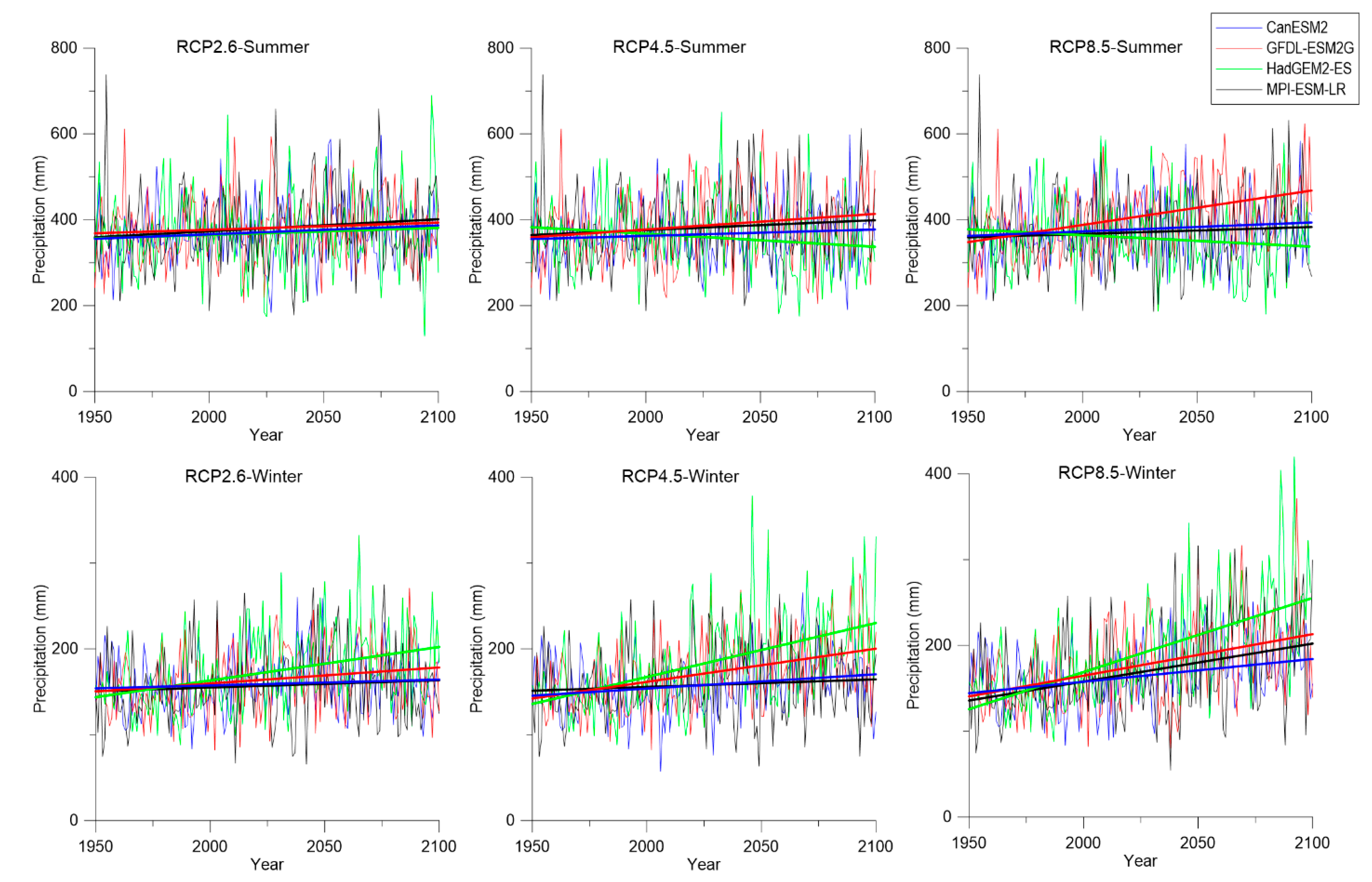
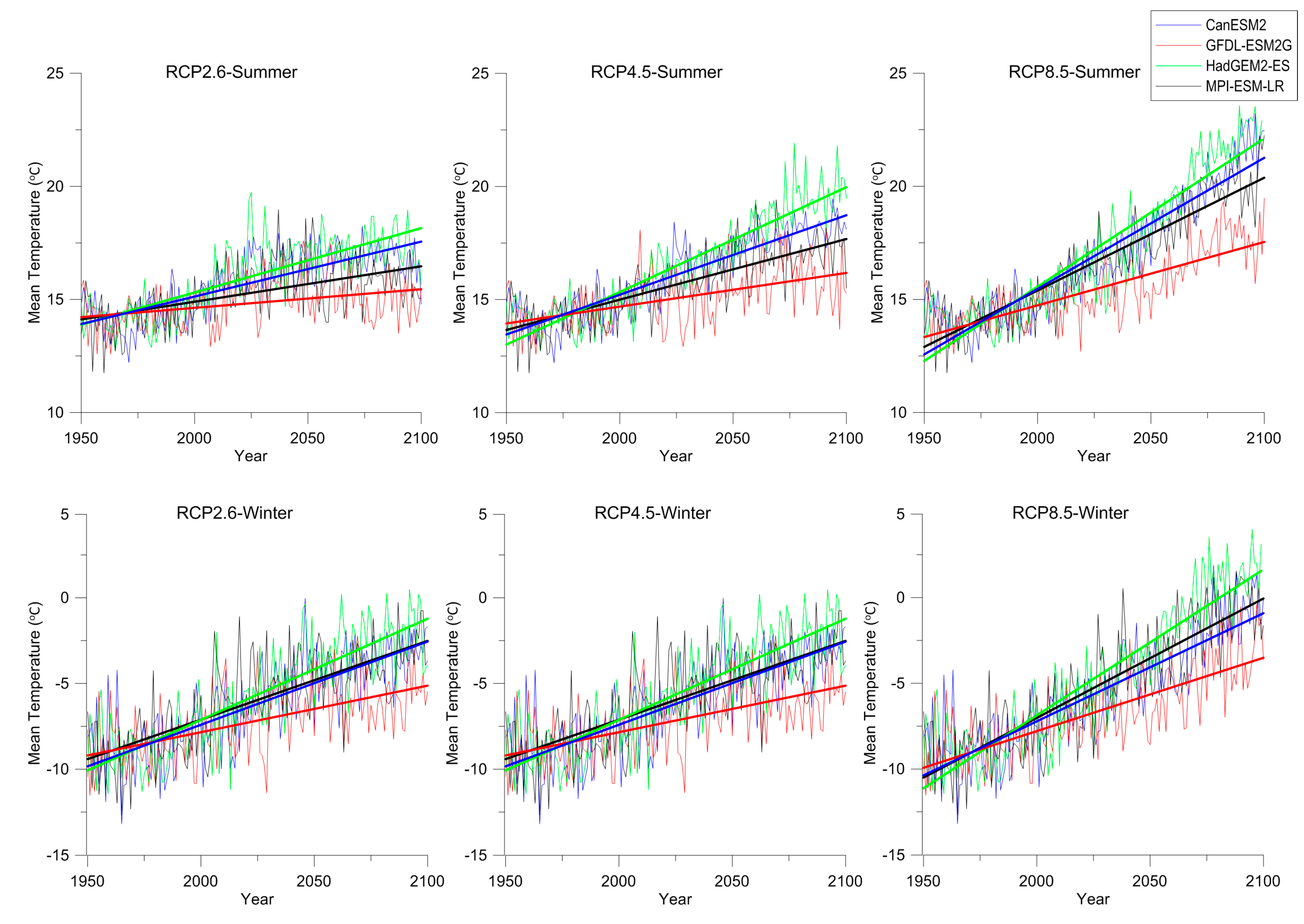
| Decade | Mean Precipitation Total (mm) | Incremental Increase % | Mean Temperature (°C) | Temperature Increase (°C) | ||||||||
|---|---|---|---|---|---|---|---|---|---|---|---|---|
| RCP | RCP | RCP | RCP | |||||||||
| 2.6 | 4.5 | 8.5 | 2.6 | 4.5 | 8.5 | 2.6 | 4.5 | 8.5 | 2.6 | 4.5 | 8.5 | |
| Summer (May–October) | ||||||||||||
| 2005–2014 | 371.9 | 371.9 | 371.9 | - | - | - | 15.29 | 15.44 | 15.25 | - | - | - |
| 2050–2059 | 413.3 | 376.8 | 377.7 | 11.1 | 1.3 | 1.56 | 16.17 | 16.86 | 17.56 | 0.9 | 1.4 | 2.3 |
| 2090–2099 | 382.2 | 381.2 | 408.9 | 2.77 | 2.5 | 9.95 | 16.00 | 17.82 | 20.51 | 0.7 | 2.4 | 5.3 |
| Winter (November–April) | ||||||||||||
| 2005–2014 | 162.7 | 162.7 | 162.7 | - | - | - | −6.867 | −6.525 | −6.857 | - | - | - |
| 2050–2059 | 174.5 | 176.9 | 199.3 | 7.25 | 8.8 | 22.5 | −5.786 | −4.489 | −4.241 | 1.1 | 2.0 | 2.6 |
| 2090–2099 | 159.6 | 189.6 | 218.7 | −1.91 | 16.6 | 34.4 | −6.158 | −3.178 | −0.430 | 0.7 | 3.4 | 6.4 |
| Year | Difference in Crop Gross Margins without Irrigation and Crop Gross Margins with Irrigation and Associated Variable and Infrastructure Costs ($/hectare) | Increase in Crop Gross Margins under Irrigation ($/hectare) | ||||
|---|---|---|---|---|---|---|
| RCP2.6 | RCP4.5 | RCP8.5 | RCP2.6 | RCP4.5 | RCP8.5 | |
| 2050 | −174.00 | −172.00 | −173.00 | −13.60 | −11.80 | −12.30 |
| 2051 | −145.00 | −151.00 | −150.00 | 15.10 | 9.42 | 10.60 |
| 2052 | −155.00 | −153.00 | −153.00 | 4.79 | 7.31 | 6.94 |
| 2053 | −150.00 | −146.00 | −147.00 | 9.99 | 14.50 | 12.80 |
| 2054 | −146.00 | −143.00 | −144.00 | 14.01 | 17.40 | 16.50 |
| 2055 | −159.00 | −159.00 | −159.00 | 0.83 | 1.53 | 1.53 |
| 2056 | −157.00 | −146.00 | −147.00 | 3.60 | 14.00 | 13.50 |
| 2057 | −143.00 | −136.00 | −142.00 | 17.40 | 24.50 | 17.90 |
| 2058 | −125.00 | −127.00 | −127.00 | 35.40 | 33.10 | 33.70 |
| 2059 | −126.00 | −126.00 | −126.00 | 33.90 | 33.90 | 33.90 |
| Average | −148.00 | −146.00 | −147.00 | 12.10 | 14.40 | 13.50 |
| Year | Difference in Crop Gross Margins without Irrigation and Crop Gross Margins with Irrigation and Associated Variable and Infrastructure Costs ($/hectare) | Increase in Crop Gross Margins under Irrigation ($/hectare) | ||||
|---|---|---|---|---|---|---|
| RCP2.6 | RCP4.5 | RCP8.5 | RCP2.6 | RCP4.5 | RCP8.5 | |
| 2090 | −173.00 | −173.00 | −174.00 | −13.10 | −13.20 | −13.50 |
| 2091 | −151.00 | −150.00 | −142.00 | 9.42 | 10.10 | 18.00 |
| 2092 | −154.00 | −154.00 | −155.00 | 6.39 | 6.35 | 4.86 |
| 2093 | −146.00 | −147.00 | −153.00 | 14.30 | 12.80 | 7.15 |
| 2094 | −143.00 | −144.00 | −146.00 | 17.00 | 16.30 | 14.00 |
| 2095 | −159.00 | −159.00 | −159.00 | 1.53 | 1.53 | 0.82 |
| 2096 | −147.00 | −147.00 | −157.00 | 13.30 | 13.00 | 3.60 |
| 2097 | −135.00 | −142.00 | −144.00 | 25.20 | 17.90 | 16.30 |
| 2098 | −125.00 | −125.00 | −125.00 | 35.30 | 35.30 | 35.40 |
| 2099 | −126.00 | −126.00 | −129.00 | 34.10 | 33.90 | 30.90 |
| Average | −146.00 | −147.00 | −148.00 | 14.30 | 13.40 | 11.80 |
© 2017 by the authors. Licensee MDPI, Basel, Switzerland. This article is an open access article distributed under the terms and conditions of the Creative Commons Attribution (CC BY) license ( http://creativecommons.org/licenses/by/4.0/).
Share and Cite
Berry, P.; Yassin, F.; Belcher, K.; Lindenschmidt, K.-E. An Economic Assessment of Local Farm Multi-Purpose Surface Water Retention Systems under Future Climate Uncertainty. Sustainability 2017, 9, 456. https://doi.org/10.3390/su9030456
Berry P, Yassin F, Belcher K, Lindenschmidt K-E. An Economic Assessment of Local Farm Multi-Purpose Surface Water Retention Systems under Future Climate Uncertainty. Sustainability. 2017; 9(3):456. https://doi.org/10.3390/su9030456
Chicago/Turabian StyleBerry, Pamela, Fuad Yassin, Kenneth Belcher, and Karl-Erich Lindenschmidt. 2017. "An Economic Assessment of Local Farm Multi-Purpose Surface Water Retention Systems under Future Climate Uncertainty" Sustainability 9, no. 3: 456. https://doi.org/10.3390/su9030456