Risk Assessment for Distribution Systems Using an Improved PEM-Based Method Considering Wind and Photovoltaic Power Distribution

Abstract

The intermittency and variability of permeated distributed generators (DGs) could cause many critical security and economy risks to distribution systems. This paper applied a certain mathematical distribution to imitate the output variability and uncertainty of DGs. Then, four risk indices—EENS (expected energy not supplied), PLC (probability of load curtailment), EFLC (expected frequency of load curtailment), and SI (severity index)—were established to reflect the system risk level of the distribution system. For the certain mathematical distribution of the DGs’ output power, an improved PEM (point estimate method)-based method was proposed to calculate these four system risk indices. In this improved PEM-based method, an enumeration method was used to list the states of distribution systems, and an improved PEM was developed to deal with the uncertainties of DGs, and the value of load curtailment in distribution systems was calculated by an optimal power flow algorithm. Finally, the effectiveness and advantages of this proposed PEM-based method for distribution system assessment were verified by testing a modified IEEE 30-bus system. Simulation results have shown that this proposed PEM-based method has a high computational accuracy and highly reduced computational costs compared with other risk assessment methods and is very effective for risk assessments.

1. Introduction

The extensive penetration of renewable-type distributed generators (DGs) (e.g., wind and PV) in distribution networks could bring many benefits to the grid, as they are alternative to conventional generators [1,2]. However, the randomness of these DGs could cause some critical risks to security and economy aspects of distribution systems, such as power quality and stability, fault level, and the value of load curtailment, which impose challenges when planning distribution systems [3,4]. Therefore, it is becoming increasingly important to assess the risks associated with the variability and uncertainty of DGs.

In the past decade, many researches concentrated on how to assess the impacts of random DGs on distribution systems. Many risk indices have been established in [5,6,7,8]. These papers aimed to establish the risk indices by using the product of probability and severity, but ignored many significant aspects such as the value of load curtailment. Many other risk indices have also been presented. In [9], three risk indices—including LOLP (loss of load probability), EENS (expected energy not supplied), and ECOST (expected customer interruption cost)—were used for reliability and price risk assessment. In [10,11], the indices of SAIFI (system average interruption frequency index), SAIDI (system average interruption duration index), and EENS were used to assess the reliability of an active distribution network. In [12], EENS, ENLC (expected number of load curtailment), and ADLC (average duration of load curtailment) were used for power system reliability assessment. In [13,14,15], EENS, PLC (probability of load curtailment), EFLC (expected frequency of load curtailment), and SI (severity index) were presented as risk indices to assess the risk level of distribution system. In [9,10,11,12,13,14,15], more considerations were concentrated on the operation risk level. Needless to say, EENS, PLC, EFLC, and SI are the most important risk indices that reflect the high penetration of DGs in distribution system.

The output uncertainties of DGs can be dealt with by many uncertainty modeling methods including probabilistic methods and other uncertainty methods [16]. Among the other uncertainty methods, IGDT (information gap decision theory), robust optimization, and a hybrid possibilistic–probabilistic approach were respectively introduced in [17,18,19]. However, the power output of wind or photovoltaic (PV) generating units is generally subject to a certain mathematical distribution [20,21]. Namely, the randomness of wind and PV can be imitated by some mathematical formulas. Therefore, these other uncertainty methods mentioned are not applicable for the risk assessment of a distribution system with the penetration of probabilistic DGs. For probabilistic DGs, probabilistic methods—including the Monte Carlo method, scenario-based decision-making method, and point estimate method—can be suitably applied. However, the Monte Carlo method (which was introduced in [22,23]) and the scenario-based decision-making method (introduced in [24]) are all computationally harder. Compared to the other probabilistic methods, the point estimate method (PEM), described in [25,26,27], has highly reduced computational costs and is extremely applicable for the probabilistic uncertainties of DGs. However, the accuracy of PEM is very low. Therefore, the traditional PEM should be improved for application.

In this study, in order to reasonably assess the risks of distribution systems with the penetration of DGs, a risk assessment method for distribution systems using an improved PEM-based method—considering wind and photovoltaic power distribution—was proposed. Four risk indices (EENS, PLC, EFLC, and SI) were applied to reflect the system risk level of distribution systems. Then, for the certain mathematical distribution of the DGs’ output power, an improved PEM-based method was proposed to calculate these four system risk indices. In this improved PEM-based method, an enumeration method was used to list the states of the distribution system; an improved PEM was proposed to deal with the uncertainties of DGs in the distribution system. Finally, the effectiveness and advantage of this proposed PEM-based method for power system assessment were verified by testing a modified IEEE 30-bus system, which showed that this proposed PEM-based method is very effective for risk assessments in distribution systems and has a high computational accuracy and largely reduced computational costs compared with other risk assessment methods. Simulation results also demonstrate that total generation capacity, type, location, dispersion, and capacity proportion of DGs have great influences on the system risk indices.

2. Distribution of Wind and Photovoltaic DGs

In distribution systems, the output of DGs contributes to whether the load can be supplied when malfunction occurs. Therefore, the output randomness of DGs should be imitated by mathematical formulas. In this paper, wind generators and photovoltaic generators are only considered as DGs.

2.1. Output Uncertainty of Wind Generators

Large amounts of research in the past decades have demonstrated that wind speed v is the main stochastic factor that determines the output power of wind generators. Generally, a Weibull distribution can be used to imitate the stochastic wind speed v [6]. The probability density function (PDF) for wind speed v is described as (1):

$$f_v(v)=\frac{k}{c}(\frac{v}{c})\exp [-{(\frac{v}{c})}^k]$$

(1)

where k and c are, respectively, the shape parameter and the scale parameter of the wind speed distribution. According to the historical data of wind speed v, these two indices can be estimated.

Based on the PDF of wind speed v, the output of a wind turbine generator can be acquired [28]:

$$P_w=\{\begin{array}{c}0,\\ P_N\frac{v-v_{in}}{v_N-v_{in}},\\ P_N,\\ 0,\end{array}\begin{array}{c}v<v_{in}\\ v_{in}\le v<v_N\\ v_N\le v<v_{out}\\ v\ge v_{out}\end{array}$$

(2)

where P_w is the active output power, P_N is the rated output power of wind turbine generator, v_N is rated wind speed, v_in is cut-in wind speed, and v_out is cut-out wind speed.

2.2. Output Uncertainty of Photovoltaic Generators

In most occasions, illumination intensity is thought to be the major factor that affects the active output of photovoltaic generators. Because of cloud cover and other insolation-reducing phenomena, the illumination intensity I can also be represented by a random variable. In general, illumination intensity I approximately follows a beta distribution with shape indexes α and β [29]:

$$f(I)=\frac{\mathsf{\Gamma }(\alpha +\beta )}{\mathsf{\Gamma }(\alpha )\mathsf{\Gamma }(\beta )}\cdot {\left(\frac{I}{I_{\max }}\right)}^{\alpha -1}\cdot {\left(1-\frac{I}{I_{\max }}\right)}^{\beta -1}$$

(3)

where I_max is the maximum intensity during a certain interval. The two shape indexes α and β can be evaluated by the mean value and the variance of illumination intensity.

Many studies have showed that the active output of photovoltaic generators could be described as [30]:

$$P_v=A\cdot \eta \cdot I$$

(4)

where A is photoelectric array area and η is the photoelectric transformation efficiency. Combining Equations (3) and (4), the PDF of photovoltaic generators’ output power P_v can be acquired:

$$f(P_v)=\frac{\mathsf{\Gamma }(\alpha +\beta )}{A\cdot \eta \cdot \mathsf{\Gamma }(\alpha )\mathsf{\Gamma }(\beta )}\cdot {\left(\frac{P_v}{P_v^{\max }}\right)}^{\alpha -1}\cdot {\left(1-\frac{P_v}{P_v^{\max }}\right)}^{\beta -1}$$

(5)

where $P_v^{\max }$ is the maximum value of P_v, which can be calculated by $P_v^{\max }$ = A·η·I_max. According to (5), P_v also follows beta distribution with shape indexes α and β.

3. Risk Assessment Indices and Method

3.1. Risk Assessment Indices

It should be noted that risk indices such as EENS, PLC, EFLC, and SI in [13,14,15] are more considered with the penetration of DGs. Therefore, in this paper, these four risk indices were used to reflect the system risk level of distribution systems. The calculation methods of these four risk indices are illustrated by the following [13]:

(1) EENS (unit: MWh/y) represents the energy that is not supplied with the penetration of DGs in the distribution system, which can be computed by (6):

$$\mathrm{EENS}={\displaystyle \sum _{i=1}^{N_L}({\displaystyle \sum _{s\in Q_i}{p}_T(s)}\cdot C_0(s))}\cdot T_i$$

(6)

where i is the load level, N_L is the set for load levels, T_i is the duration of i, and Q_i is the set for system state s at load level i. p_T(s) and C₀(s) are, respectively, the occurrence probability and total load curtailment of system state s.

(2) PLC can be calculated by:

$$\mathrm{PLC}={\displaystyle \sum _{i=1}^{N_L}({\displaystyle \sum _{s\in Q_i}{p}_T(s)})}\cdot \frac{T_i}{T}$$

(7)

(3) EFLC (unit: times/y) can be calculated by:

$$\mathrm{EFLC}={\displaystyle \sum _{i=1}^{N_L}{\displaystyle \sum _{s\in Q_i}\left(p_T(s){\displaystyle \sum _{j=1}^{m(s)}{\theta }_j}\right)}}\cdot \frac{T_i}{T}$$

(8)

where T is total duration of T_i and m(s) is the set of component j at system state s. For component j, θ_j represents transfer rate of component j, which is equal to repair rate ${\mu }_j$ in this paper.

(4) SI (unit: min/y) represents the equivalent duration under an entire system outage during peak conditions, which can be calculated:

$$\mathrm{SI}=\frac{\mathrm{EENS}\times 60}{L}$$

(9)

where L is the value of peak load in 1 year.

In these four risk indices, SI is closely related to EENS. In order to calculate the index of EENS, the total load curtailment at state s C₀(s) should be calculated beforehand; this can be calculated by optimal power flow (OPF), introduced in Section 3.3. For all of these four risk indices, the occurrence probability of system state s p_T(s) is needed. Therefore, an enumeration method is applied for system state selection, which is introduced in Section 4.2.

3.2. Improved Point Estimate Methods

Point estimate method (PEM), which was firstly proposed by Hong in 1998, focuses on the statistical information that is provided by the first few central moments of the input random variables [25]. For each variable, K points are used, and K is a parameter named concentrations and depends on the Hong’s method. These points and the function—which relates input and output variables—are used to obtain the information about the uncertainty associated with problem output random variables.

This paper relies on a 2m and 2m + 1 type scheme of PEM for computing the four risk indices described in Section 3.1, which gives a good trade-off between the solution accuracy and the computational efforts. m denotes the number of random variables, which are wind speed v or illumination intensity I. The 2m type scheme of PEM uses the first two concentrations for each input random variable (i.e., K = 2). For the 2m + 1 type scheme of PEM, K = 3.

Generally speaking, PEM is used to calculate the estimation value (Z^j) of F(X) (Z = F(X) = F(X₁, X₂, …, X_m)) when the stochastic numerical characteristics of variables X₁, X₂, …, X_m are known [26,27]. The point estimation principle can be depicted as:

$$𝔼(Z^j)\approx {\displaystyle \sum _{l=1}^m{\displaystyle \sum _{k=1}^K{\omega }_{l,k}{F}^j({\mu }_{X1},\cdots ,x_{l,k},\cdots ,{\mu }_{Xm})}}$$

(10)

where j is the power of F(X), m is the number of DGs, ${\mu }_{Xi}$ and ξ_i,k are, respectively, the expectation and standard location of variable X_i, which represents illumination intensity I or wind speed v in this paper. ω_l,k represents the weight of X_i at x_l,k, which can be calculated by (11):

$$x_{i,k}={\mu }_{X_i}+{\xi }_{i,k}{\sigma }_{X_i},i=1,2,\cdots ,m;k=1,2,\cdots ,2K-1$$

(11)

where ${\sigma }_{Xi}$ represents the variance of X_i. Standard location ξ_i,k and weight ω_l,k could be determined by (12):

$$\{\begin{array}{c}{\displaystyle \sum _{k=1}^K{\omega }_{i,k}\cdot {\xi }_{i,k}{}^j}={\lambda }_{i,j},j=1,\cdots ,2K-1\\ {\lambda }_{i,j}=E\left[{(x_i-{\mu }_{X_i})}^j\right]/{\sigma }_{X_i}{}^j\\ {\displaystyle \sum _{k=1}^K{\omega }_{i,k}}={\alpha }_i\end{array}$$

(12)

In traditional PEM, ${\displaystyle \sum _{k=1}^K{\omega }_{i,k}}$ is set as $\frac{1}{m}$, which means the impacts of X_i on Z are the same. This assumption can simplify the calculation but may cause a big computational error as there are different impacts of X_i on Z. In the improved PEM, ${\displaystyle \sum _{k=1}^K{\omega }_{i,k}}$ is set as ${\alpha }_i$, which can be determined by the analytic hierarchy process (AHP) described in [31] or the contribution of X_i on Z. This equation appears to be more reasonable, as it considers the different impacts of X_i on Z.

When K = 2 and ξ_i,3 = 0, the equation of (12) can be solved:

$$\{\begin{array}{c}{\xi }_{i,1}=\frac{{\lambda }_{i,3}}{2}+\sqrt{\frac{1}{{\alpha }_i}+{(\frac{{\lambda }_{i,3}}{2})}^2},{\xi }_{i,2}=\frac{{\lambda }_{i,3}}{2}-\sqrt{\frac{1}{{\alpha }_i}+{(\frac{{\lambda }_{i,3}}{2})}^2}\\ {\omega }_{i,1}=-\frac{{\alpha }_i\cdot {\xi }_{i,2}}{{\xi }_{i,1}-{\xi }_{i,2}},{\omega }_{i,2}=\frac{{\alpha }_i\cdot {\xi }_{i,1}}{{\xi }_{i,1}-{\xi }_{i,2}}\end{array}$$

(13)

The calculation results based on (13) is named 2m improved PEM. When K = 3 and ξ_i,3 = 0, 2m + 1 improved PEM can be constructed, and the solving results of Equation (12) are:

$$\{\begin{array}{c}{\xi }_{i,1}=\frac{{\lambda }_{i,3}}{2}+\sqrt{{\lambda }_{i,4}-\frac{3}{4}{\lambda }_{i,3}{}^2},{\xi }_{i,2}=\frac{{\lambda }_{i,3}}{2}-\sqrt{{\lambda }_{i,4}-\frac{3}{4}{\lambda }_{i,3}{}^2}\\ {\omega }_{i,1}=\frac{1}{{\xi }_{i,1}({\xi }_{i,1}-{\xi }_{i,2})},{\omega }_{i,2}=-\frac{1}{{\xi }_{i,2}({\xi }_{i,1}-{\xi }_{i,2})}\\ {\omega }_{i,3}={\alpha }_i-\frac{1}{{\lambda }_{i,4}-{\lambda }_{i,3}{}^2}\end{array}$$

(14)

The AHP is a rough estimation of weights and may be complex in operation. Therefore, the contribution of X_i on Z which can be approximated by the capacity proportion of DG i was used to calculate the value of α_i.

According to Equations (10)–(14), the j-th raw moment of the output random vector Z can be acquired. Then, the mean and the standard deviation of Z can be estimated by Equation (15):

$${\mu }_Z=𝔼(Z)\approx {\displaystyle \sum _{l=1}^m{\displaystyle \sum _{k=1}^K{\omega }_{l,k}F({\mu }_{X1},\cdots ,x_{l,k},\cdots ,{\mu }_{Xm})}},{\sigma }_Z=\sqrt{E(Z^2)-{\mu }_Z{}^2}$$

(15)

For each risk assessment index, the mean and the standard deviation can be respectively acquired by Equation (15). For a variable with a certain mathematical distribution, the mean is the most probable value of the variable [26]. Therefore, the mean of Z, ${\mu }_Z$, is used as the estimation value of each risk index in this paper.

3.3. Optimal Power Flow Algorithm in Distribution Systems

In distribution systems, load curtailment and generation dispatch are extensively applied to enable the system to go from urgent state to normal state. In order to obtain the system security indices in distribution systems, an optimal power flow (OPF) algorithm was presented in this paper to assess the total load curtailment C₀(s) in state s. Equations (16) and (17) were used in the optimal power flow algorithm to simulate the curtailment and dispatch work and ensure the security of distribution system [32]:

$$\min f(\Delta P_{G1},\cdots ,\Delta P_{Gm},\Delta P_{L1},\cdots ,\Delta P_{Ll})={\displaystyle \sum _{k=1}^m{C}_{Gk}\Delta P_{Gk}}+{\displaystyle \sum _{h=1}^l{C}_{Lh}\Delta P_{Lh}}$$

(16)

$$\begin{array}{ll}s.t.& {\displaystyle \sum _{k=1}^m\frac{\partial I_{ij}}{\partial P_{Gk}}\Delta P_{Gk}}+{\displaystyle \sum _{h=1}^l\frac{\partial I_{ij}}{\partial P_{Lh}}\Delta P_{Lh}}\le I_{ij}^{\max }-I_{ij}^0\\ & {\displaystyle \sum _{k=1}^m\frac{\partial P_s}{\partial P_{Gk}}\Delta P_{Gk}}+{\displaystyle \sum _{h=1}^l\frac{\partial P_s}{\partial P_{Lh}}\Delta P_{Lh}=0}\\ & P_{Gk}^{\min }-P_{Gk}^0\le \Delta P_{Gk}\le P_{Gk}^{\max }-P_{Gk}^0\\ & 0\le \Delta P_{Lh}\le P_{Lh}^0\\ & 1\le k\le m,1\le h\le l,1\le i\le N_b,1\le j\le N_b\end{array}$$

(17)

where l is the number of load buses in distribution systems. $\frac{\partial z}{\partial x}(z=I_{ij},P_s;x=P_{Gk},P_{Lh})$ are sensitivity coefficients. N_b is the number of buses; ΔP_Gk and ΔP_Lh are respectively the power variations of generator k and load h; C_GK and C_Lh are respectively the control cost of generator k and load h; and I_ij is the current through overload line ij.

According to the results of this optimal power flow algorithm in distribution systems, the total load curtailment in state s, C₀(s), can be calculated by Equation (18):

$$C_0\left(s\right)={\displaystyle \sum _{h=1}^l\Delta P_{Lh}}+\Delta P_d$$

(18)

where ΔP_d is the value of load curtailment caused by direct structure change of the distribution system. In line with the values of C₀(s) and p_T(s), the risk assessment indices in Equations (6)–(9) can be calculated.

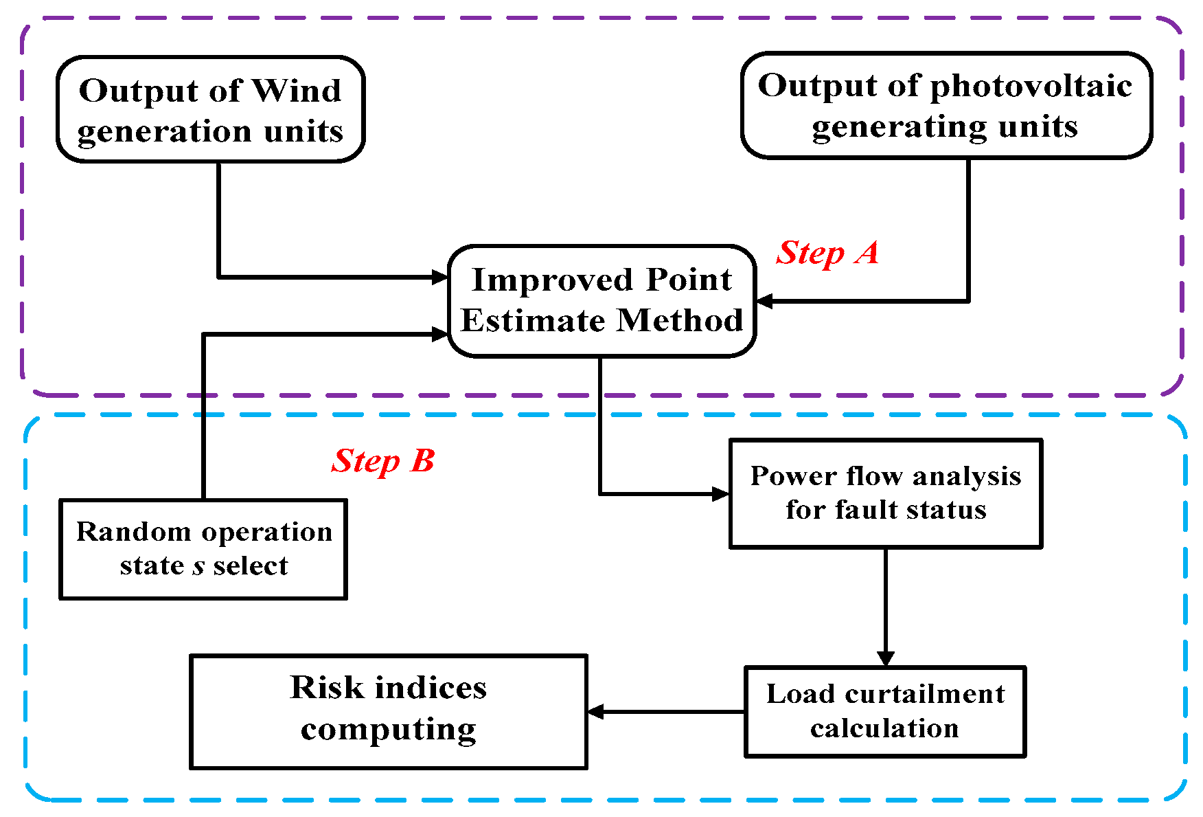
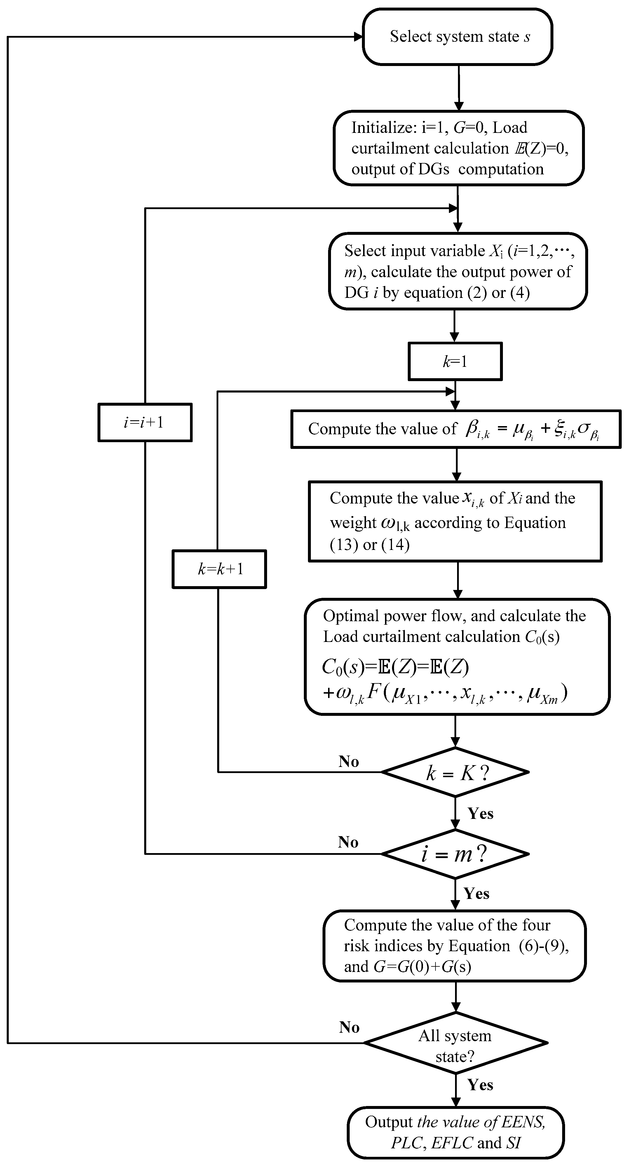
4. Risk Assessment Procedure for Distribution Systems

4.1. Structure for Risk Assessment

To assess the four risk indices in distribution systems, PEM was used and the uncertainties of distribution generators were sufficiently considered. The flowchart of the improved PEM-based method for risk assessment of distribution systems is shown in Figure 1.

In Step A, active outputs of photovoltaic generators and wind generators are calculated according to the stochastic wind speed v and illumination intensity I. In step B, random operation state s of the distribution system was firstly selected. Then, optimal power flow algorithm in state s was applied to compute the value of load curtailment based on the improved point estimate method. Then, the four risk indices listed in Section 3.1 were computed until all the random operation states s are considered.

4.2. Procedure for Calculating Risk Indices

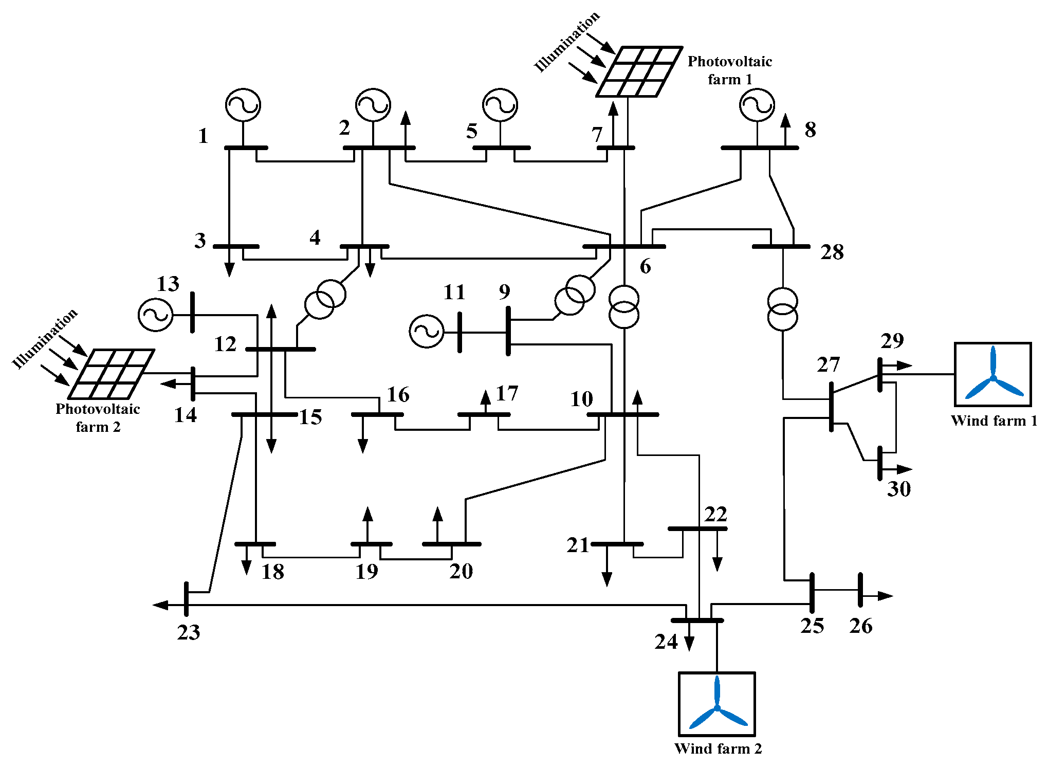
In [13], according to DGs’ probability model, the indices of EENS, PLC, EFLC, and SI were calculated by a proposed hierarchical risk assessment method, which is the combination of a Monte Carlo simulation and an enumeration method. However, this proposed hierarchical method is relatively complex in application. In [6], 2m + 1 PEM was utilized to assess the overload risk of a transmission line. This 2m + 1 PEM has lower accuracy compared to a Monte Carlo simulation. However, the computational burden of 2m + 1 PEM is greatly reduced. Consequently, the improved PEM is applied to compute the four risk indices in this paper. For comparison, the calculation results of the four risk indices based on the hierarchical risk assessment method in [13] were used as the exact values, and the error in accuracy of the improved PEM-based method for risk assessment was analyzed.

For convenience, symbol G is used to represent any parameter of the four risk indices including EENS, PLC, EFLC, and SI. Namely, to calculate the parameter G is to calculate these four risk indices. The designed procedure for computing the symbol G based on PEM is summarized as Figure 2.

In Figure 2, 2m and 2m + 1 improved-PEM were used, respectively. The output power of DG i is calculated by Equation (2) or (4). Further, OPF was applied to calculate the value of C₀(s), which can be referred from Equations (16) and (17). The detailed procedure of the improved PEM-based method for computing risk indices G is summarized as follows.

Step (1): Enumeration method is used to list the states of the distribution system. The occurrence probability p_T(s) in system state s can be calculated by Equation (19):

$$p_T(s)={\displaystyle \prod _{i=1}^{N_f}{\frac{{\lambda }_i}{{\lambda }_i+{\mu }_i}}_i}{\displaystyle \prod _{j=1}^{N_n}(1-\frac{{\lambda }_j}{{\lambda }_j+{\mu }_j})}$$

(19)

where N_f is the total number of failure components, N_n is the total number of normal components. For component i, ${\mu }_i$ is the repair rate, ${\lambda }_i$ is the outage rate, and these two parameters can be obtained by statistics.

Step (2): Initialize and generate the constructed points of wind speed v as well as illumination intensity I. Initialize the initial value of load curtailment calculation 𝔼(Z) = 0 and the initial value of G = 0.

Step (3): Construct the parameters of improved point estimate method, which contains the following substeps:

1) Select the input variable X_i (i = 1, 2, …, m). For wind generating unit i, X_i represents the stochastic wind speed v; for photovoltaic generating units i, X_i represents the stochastic illumination intensity I. m is the total number of wind generators and photovoltaic generators. Then, the output power of DG i is calculated by Equation (2) or (4).

2) With the first central moments, standard locations ξ_i,k and the weights ω_l,k for random variables are computed by Equation (12) or (13). Then, the concentrations x_i,k can be calculated by Equation (10). Consequently, the point (μ_x1, μ_x2, …, x_i,k, …, μ_xm) is constructed.

3) Based on the output of DG i, optimal power flow in state s is applied to compute the value of C₀(s) according to Equations (15) and (16).

4) Repeat sub-steps 2–3 until variable k reaches K. For 2m improved PEM, K = 2; for 2m + 1 improved PEM, K = 3.

5) Repeat sub-steps 2–4 until variable i reaches the total number m, and the calculation of G in state s is completed.

Step (4): Repeat Steps (1)–(3) until all the states in distribution system are considered.

Step (5): Output the values of the four risk indices EENS, PLC, EFLC, and SI.

5. Case Studies

In order to verify the rationality of the proposed PEM-based method for risk assessment of a distribution system, IEEE 30-bus system with DGs is applied, as shown in Figure 3. For all nodes, the upper voltage bound is 1.06 p.u. and lower voltage bound is 0.94 p.u. in this paper [6]. All the cases are achieved by MATLAB in an Advanced Micro Devices 64 Dual Core 3.3 GHz PC. For photovoltaic farms, shape indexes α = 15.42, β = 4.3, A = 2.17 m, η = 13.53%. For wind farms, rated wind speed v_N = 15 m/s, cut-in wind speed v_in = 4m/s, cut-out wind speed v_out = 20 m/s, shape index k = 6.23, and scale index c = 10.43.

5.1. Calculation of Risk Indices Based on PEM

In this modified IEEE 30-bus system, two wind farms and two photovoltaic farms are connected to nodes 7, 14, 24, and 29. The capacity proportion of these four farms is 20%:30%:20%:30%. However, the ratio of DGs’ total generation capacity to the total load K_d varies from 0 to 1. With the known capacity proportion of DGs, the value of α_i can be obtained: α₁ = 0.2, α₂ = 0.3, α₃ = 0.2, α₄ = 0.3.

According to the designed procedure for computing risk indices in Figure 2 and the parameters of DGs, the calculation results of EENS, PLC, EFLC, and SI, based on 2m and 2m + 1 improved PEM, are listed in

Table 1. Calculation results of risk indices based on 2m improved PEM.

Kd	2m PEM
	EENS (MWh/y)	PLC	EFLC (Times/y)	SI (min/y)
0	3151.2	62,247 × 10−7	2.4899	66.716
0.2	2382.5	59,981 × 10−7	2.3992	50.441
0.4	1945.7	53,176 × 10−7	2.1285	41.193
0.6	1744.4	48,635 × 10−7	1.9454	36.932
0.8	1619.1	47,516 × 10−7	1.9006	34.279
1	1580.3	45,243 × 10−7	1.8097	33.457

K_d: generation capacity; EENS: expected energy not supplied; PLC: probability of load curtailment; EFLC: expected frequency of load curtailment; SI: severity index.

and

Table 2. Calculation results of risk indices based on 2m + 1 improved PEM.

Kd	2m + 1 PEM
	EENS (MWh/y)	PLC	EFLC (Times/y)	SI (min/y)
0	3156.7	62,293 × 10−7	2.4917	66.832
0.2	2385.4	60,033 × 10−7	2.4013	50.502
0.4	1948.2	53,212 × 10−7	2.1285	41.246
0.6	1747.3	48,687 × 10−7	1.9475	36.993
0.8	1621.8	47,551 × 10−7	1.9020	34.336
1	1582.5	45,285 × 10−7	1.8114	33.504

, respectively.

As can be seen from Table 1 and Table 2, with the increase of total generation capacity K_d, all of these risk indices decrease gradually. When the generation capacity K_d = 0, which means that DGs are not permeated, the value of EENS is about 3156.7 MWh/year. However, EENS decreases by nearly a half and drops to about 1582.5 MWh/year when the generation capacity K_d rises to 1. Analogously, the value of PLC decreases from about 0.0062293 to 0.0045285 when generation capacity K_d rises from 0 to 1.

The variation tendency of SI is consistent with the variation tendency of EENS since the index of SI is calculated by EENS, which is shown in Section 3.1. Similarly, the variation tendency of EFLC is consistent with the variation tendency of PLC. In addition, the calculation results of risk indices based on 2m improved PEM are very close with the calculation results of risk indices based on 2m + 1 improved PEM.

From Table 1 and Table 2, EENS and SI decrease smoothly with the increment of generation capacity K_d. In addition, the slope of EENS and SI decreases with the growth of generation capacity K_d. Therefore, the decreasing trend of EENS and SI is not as tangible as before, decreasingly when generation capacity K_d increases.

As shown in Table 1 and Table 2, the decrease of EENS, PLC, ELIC, and SI slows when generation capacity K_d increases to about 0.6. Namely, a large value of K_d that promotes the decrease of risk indices of distribution systems is not significantly remarkable. However, the consumption of wind and photovoltaic energy becomes an increasing problem with the increasing generation capacity K_d. It is with reluctance that too much wind and photovoltaic power is abandoned in distribution systems. Therefore, it is not necessary to increase the value of K_d to a certain large degree.

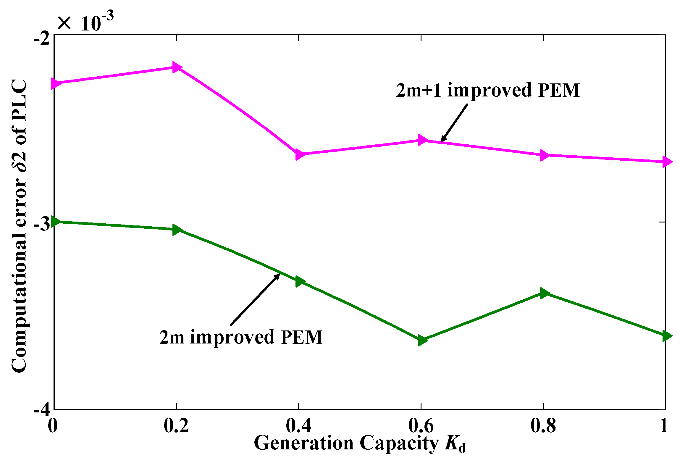
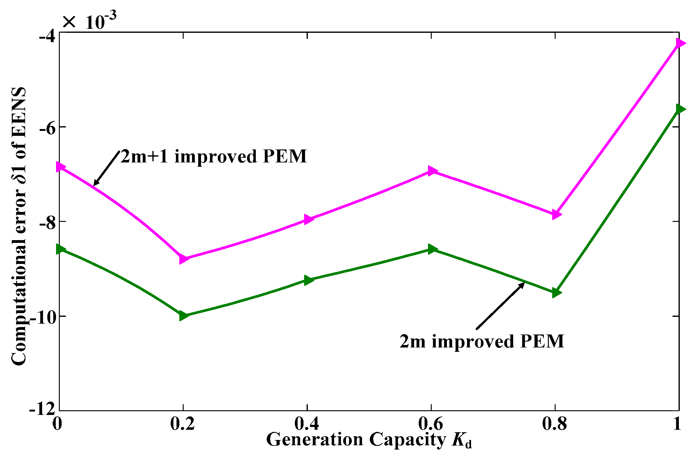
5.2. Deviation and Computational Cost Comparison

In order to illustrate the effectiveness of this improved PEM-based method for risk assessment in distribution systems, the calculation results of EENS, PLC, EFLC, and SI are shown in

Table 3. Calculation results of risk indices based on hierarchical risk assessment method.

Kd	Hierarchical Method
	EENS (MWh/y)	PLC	EFLC (Times/y)	SI (min/y)
0	3178.5	62,434 × 10−7	2.4974	67.293
0.2	2406.6	60,164 × 10−7	2.4066	50.95
0.4	1963.8	53,353 × 10−7	2.1341	41.577
0.6	1759.5	48,812 × 10−7	1.9525	37.251
0.8	1634.6	47,677 × 10−7	1.9071	34.608
1	1589.2	45,407 × 10−7	1.8163	33.646

.

Comparing the calculation results of risk indices in Table 1 and Table 2 with Table 3, it can be seen that they are very close in value. However, the calculation results of these improved PEM-based methods are all less than that of the hierarchical risk assessment method since PEM is an order approximation, which ignores the higher-order terms. Besides, the calculation results of 2m + 1 improved PEM are closer to the exact value than the calculation results of 2m improved PEM, as 2m improved PEM is a third-order approximation but 2m + 1 improved PEM is a fourth-order approximation, in fact.

According to the analysis in Section 3.1, the variation tendency of SI is consistent with the variation tendency of EENS, and the variation tendency of EFLC is consistent with the variation tendency of PLC. Therefore, the deviation comparison of EENS and PLC are only needed to be analyzed, which are shown in Figure 4 and Figure 5.

In Figure 4 and Figure 5, errors δ₁ and δ₂ are respectively calculated by comparing the results of EENS and PLC in Table 1 and Table 2 with Table 3. As can be seen from Figure 4 and Figure 5, the maximum value of computational error δ₁ is about 0.99% and the maximum value of computational error δ₂ is about 0.37%. The computational errors δ₁ and δ₂ are all less than 1%, which greatly verifies the effectiveness of this improved PEM-based method for risk assessment of distribution systems. Also, the computational error δ₂ of PLC is less than the computational error δ₁ of EENS. This is because optimal power flow algorithm (based on Equations (15) and (16)) is used in the calculation procedure for EENS.

Compared with hierarchical risk assessment method—which is a combination of the Monte Carlo method and enumeration method—in fact, the computational burden of this PEM-based method is greatly reduced. When generation capacity K_d = 0.5, the computational costs of risk indices are as listed in

Table 4. Calculation results of risk indices based on hierarchical risk assessment method.

Risk Indices	The Computational Costs of Risk Indices(s)
	2m Improved PEM	2m + 1 Improved PEM	Hierarchical Method
EENS	25.845	27.742	67.293
PLC	1.985	2.031	5.950
EFLC	2.157	2.192	6.107
SI	25.845	27.742	67.293

.

As can be seen from Table 4, the computational costs of this improved PEM-based method for risk assessment in distribution systems are much less than the computational costs of the hierarchical method. For EENS, the computational costs of 2m improved PEM and 2m + 1 improved PEM are 25.845 s and 27.742 s, respectively, but the computational cost of the hierarchical method is 67.293 s. This is because the Monte Carlo method, with many computational hurdles, is used in the hierarchical method. On the contrary, only a few numerical operations are needed in the improved PEM. The calculation of risk indices has to be evaluated only K times for each input variable, which is stochastic wind speed v or stochastic illumination intensity I at the K points.

In addition, the computational costs of 2m + 1 improved PEM-based method are almost the same compared to 2m improved PEM-based method, as the only difference between these two methods are a few numerical operations. These simulations have demonstrated that the improved PEM-based method has high accuracy and highly reduced computational costs, therefore, it is extremely applicable for risk assessment of distribution systems.

5.3. Influence of DGs on System Risk

Many researches have shown that many other aspects such as type, location, dispersion, and capacity proportion of DGs have great influences on the system risk indices. In this part, the influences of these aspects are analyzed.

In Section 5.1, two wind farms and two photovoltaic farms are connected to nodes 7, 14, 24, and 29. Suppose that four wind generating units are respectively connected to nodes 7, 14, 24, and 29 and their capacity proportion is still 20%:30%:20%:30%. This case is named case 1 in this paper. According to the developed 2m + 1 improved PEM-based method for risk assessment in Figure 2, the four system risk indices of EENS, PLC, EFLC, and SI can be acquired when generation capacity K_d = 0.2, which can be seen in

Table 5. Calculation results of risk indices in case 1.

Kd	2m + 1 Improved PEM
	EENS (MWh/y)	PLC	EFLC (Times/y)	SI (min/y)
0.2	2131.7	56,823 × 10−7	2.2729	45.131

.

As can be seen from Table 5, the index of EENS decreases from 2385.4 MWh/y to 2131.7 MWh/y and the values of other indices are also cut down distinctly. Therefore, for DGs’ type, wind farms’ power support is better than that of photovoltaic farms. These results reflect that the randomness of the output power of photovoltaic farms is even bigger than the active output power of wind farms.

To illustrate the influence of DGs’ location, suppose that two wind farms and two photovoltaic farms are respectively connected to nodes 3, 14, 19, and 30 in this part, and their capacity proportion is still 20%:30%:20%:30%. This case is named case 2 in this paper. Likewise, the calculation results of system risk indices based on 2m + 1 improved PEM, when generation capacity K_d = 0.2, are outlined in

Table 6. Calculation results of risk indices in case 2.

Kd	2m + 1 Improved PEM
	EENS (MWh/y)	PLC	EFLC (Times/y)	SI (min/y)
0.2	2193.6	57,232 × 10−7	2.2893	46.442

.

Comparing the calculation results of Table 6 with Table 2, it is observed that the index of EENS decreases from 2385.4 MWh/y to 2193.6 MWh/y and the values of other indices are also cut down distinctly. This comparison shows that the locations of nodes 3, 14, 19, and 30 are more suitable for optimal siting of DGs than nodes 7, 14, 24, and 29. However, these locations may be not the most optimal siting for DGs, and how to ascertain the optimal siting of DGs is worth further study.

To illustrate the influence of DG dispersion, suppose that three wind farms and three photovoltaic farms are respectively connected to nodes 3, 7, 14, 24, 29, and 30 in this part, and their capacity proportion is 15%:15%:20%:15%:15%:20%. This case is named case 3 in this paper and the calculation results of system risk indices are outlined in

Table 7. Calculation results of risk indices in case 3.

Kd	2m + 1 Improved PEM
	EENS (MWh/y)	PLC	EFLC (Times/y)	SI (min/y)
0.2	2058.4	55,785 × 10−7	2.2314	43.579

.

In case 3, the total proportion of wind farms and photovoltaic farms is still 50%:50% but the dispersion degree of DGs in case 3 is enhanced. The results in Table 2 and Table 7 show that system risk indices decrease along with dispersion degree increment. Therefore, when installed, DGs should be as highly dispersed as possible for the optimal siting of DGs for application.

The influence of DGs’ capacity proportion reflects the influence of DGs’ type on system risk indices. As wind farms’ power support is better than that of photovoltaic farms, the values of system risk indices are cut down when the wind generating units’ capacity proportion is increased.

These test results illustrate that appropriate DGs’ siting and sizing have great influences on the system risk indices. For the sizing of DGs, system risk indices increase along with the DG’s capacity, however, the corresponding investment costs will increase. For the appropriate siting of DGs, different locations may suit different types of DGs, and DGs’ dispersion can decrease the value of system risk indices.

6. Conclusions

DGs connected to a distribution system could cause some critical risks to distribution systems from security and economy aspects. In order to reasonably assess the risks of distribution systems with penetrating DGs, four risk indices—EENS, PLC, EFLC, and SI—were used in this paper to reflect the system risk level in distribution systems. The output uncertainties of DGs were depicted by some certain mathematical distributions. Then, an improved PEM-based method was proposed to calculate these four system risk indices. In this improved PEM-based method, enumeration method was used to list the states of distribution systems, and an improved PEM was presented to deal with the uncertainties of DGs.

Test results of case studies have shown that this proposed PEM-based method is highly effective for assessing the risk of a distribution system with DGs, as it has a high computational accuracy and highly reduced computational costs compared with other risk assessment methods. Simulation results also demonstrate that total generation capacity, type, location, dispersion, and capacity proportion of DGs have great influences on the system risk indices. The determining method of appropriate DGs’ siting and sizing, considering the operation risk of a distribution system with DGs, is worthy of further research.

References

1. Arabali, A.; Ghofrani, M.; Etezadi-Amoli, M. Stochastic Performance Assessment and Sizing for a Hybrid Power System of Solar/Wind/Energy Storage. IEEE Trans. Sustain. Energy 2014, 5, 363–371. [Google Scholar] [CrossRef]
2. Zhao, H.; Guo, S. External Benefit Evaluation of Renewable Energy Power in China for Sustainability. Sustainability 2015, 7, 4783–4805. [Google Scholar] [CrossRef]
3. Wu, Q.; Peng, C. Comprehensive Benefit Evaluation of the Power Distribution Network Planning Project Based on Improved IAHP and Multi-Level Extension Assessment Method. Sustainability 2016, 8, 796. [Google Scholar] [CrossRef]
4. Al Kaabi, S.S.; Zeineldin, H.H.; Khadkikar, V. Planning Active Distribution Networks Considering Multi-DG Configurations. IEEE Trans. Power Syst. 2014, 29, 785–793. [Google Scholar] [CrossRef]
5. Negnevitsky, M.; Nguyen, D.H.; Piekutowski, M. Risk Assessment for Power System Operation Planning with High Wind Power Penetration. IEEE Trans. Power Syst. 2015, 30, 1359–1368. [Google Scholar] [CrossRef]
6. Li, X.; Zhang, X.; Wu, L. Transmission Line Overload Risk Assessment for Power Systems with Wind and Load-Power Generation Correlation. IEEE Trans. Smart Grid 2015, 3, 1233–1242. [Google Scholar] [CrossRef]
7. Marsadek, M.; Mohamed, A.; Mohd, Z. Assessment and classification of line overload risk in power systems considering different types of severity functions. WSEAS Transcr. Power Syst. 2010, 3, 182–191. [Google Scholar]
8. Feng, Y.Q.; Wu, W.C.; Zhang, B.; Li, W.Y. Power system operation risk assessment using credibility theory. IEEE Trans. Power Syst. 2008, 23, 1309–1318. [Google Scholar] [CrossRef]
9. Ding, Y.; Wang, P. Reliability and price risk assessment of a restructured power system with hybrid market structure. IEEE Trans. Power Syst. 2006, 21, 108–116. [Google Scholar] [CrossRef]
10. Celli, G.; Ghiani, E.; Pilo, F.; Soma, G.G. Active distribution network reliability assessment with a pseudo sequential Monte Carlo method. In Proceedings of the IEEE PowerTech, Trondheim, Norway, 19–23 June 2011; pp. 1–8. [Google Scholar]
11. Atwa, Y.M.; El-Saadany, E.F. Reliability evaluation for distribution system with renewable distributed generation during islanded mode of operation. IEEE Trans. Power Syst. 2009, 24, 572–581. [Google Scholar] [CrossRef]
12. Li, W.; Zhou, J.; Lu, J.; Yan, W. Incorporating a combined fuzzyand probabilistic load model in power system reliability assessment. IEEE Trans. Power Syst. 2007, 22, 1386–1388. [Google Scholar] [CrossRef]
13. Jia, H.; Qi, W.; Liu, Z.; Wang, B. Hierarchical Risk Assessment of Transmission System Considering the Influence of Active Distribution Network. IEEE Trans. Power Syst. 2015, 2, 1084–1093. [Google Scholar] [CrossRef]
14. Li, W.; Zhou, J.; Xie, K.; Xiong, X. Power system risk assessment using a hybrid method of fuzzy set and Monte Carlo simulation. IEEE Trans. Power Syst. 2008, 23, 336–343. [Google Scholar]
15. Billinton, R.; Wang, P. Reliability cost/worth assessment ofdistribution systems incorporating time-varying weather conditions andrestorations resources. IEEE Trans. Power Deliv. 2002, 17, 260–265. [Google Scholar]
16. Soroudi, A.; Amraee, T. Decision making under uncertainty in energy systems: State of the art. Renew. Sustain. Energy Rev. 2013, 28, 376–384. [Google Scholar] [CrossRef]
17. Soroudi, A.; Ehsan, M. IGDT based robust decision making tool for DNOs in load procurement under severe uncertainty. IEEE Trans. Smart Grid 2013, 4, 886–895. [Google Scholar] [CrossRef]
18. Bertsimas, D.; Litvinov, E.; Sun, X.A.; Zhao, J.; Zheng, T. Adaptive robust optimization for the security constrained unit commitment problem. IEEE Trans. Power Syst. 2013, 28, 52–63. [Google Scholar] [CrossRef]
19. Baudrit, C.; Dubois, D.; Guyonnet, D. Joint propagation and exploitation of probabilistic and possibilistic information in risk assessment. IEEE Trans. Fuzzy Syst. 2006, 14, 593–608. [Google Scholar] [CrossRef]
20. Liu, K.Y.; Sheng, W.; Hu, L.; Liu, Y. Simplified probabilistic voltage stability evaluation considering variable renewable distributed generation in distribution systems. IET Gener. Transm. Distrib. 2015, 9, 1464–1473. [Google Scholar] [CrossRef]
21. Liu, Z.; Wen, F.; Ledwich, G. Optimal siting and sizing of distributed generators in distribution systems considering uncertainties. IEEE Trans. Power Deliv. 2011, 26, 2541–2551. [Google Scholar] [CrossRef]
22. Rei, A.M.; Schilling, M.T. Reliability assessment of the Brazilianpower system using enumeration and Monte Carlo. IEEE Trans. Power Syst. 2008, 23, 1480–1487. [Google Scholar] [CrossRef]
23. Martinez-Velasco, J.A.; Guerra, G. Parallel Monte Carlo approach for distribution reliability assessment. IET Gener. Transm. Distrib. 2014, 8, 1810–1819. [Google Scholar] [CrossRef]
24. Conejo, A.J.; Carrión, M.; Morales, J.M. Decision Making under Uncertainty in Electricity Markets; Springer: New York, NY, USA, 2010; Volume 1. [Google Scholar]
25. Hong, H.P. An efficient point estimate method for probabilistic analysis. Reliab. Eng. Syst. Saf. 1998, 59, 261–267. [Google Scholar] [CrossRef]
26. Morales, J.M.; Perez-Ruiz, J. Point estimate schemes to solve the probabilistic power flow. IEEE Trans. Power Syst. 2007, 4, 1594–1601. [Google Scholar] [CrossRef]
27. Su, C.L. Probabilistic load-flow computation using point estimate method. IEEE Trans. Power Syst. 2005, 20, 1843–1851. [Google Scholar] [CrossRef]
28. Papavasiliou, A.; Oren, S.S.; O’Neill, R.P. Reserve requirements for wind power integration: A scenario-based stochastic programming framework. IEEE Trans. Power Syst. 2011, 26, 2197–2206. [Google Scholar] [CrossRef]
29. Li, J.; Wei, W.; Xiang, J. A simple sizing algorithm for stand-alone PV/wind/battery hybrid microgrids. Energies 2012, 5, 5307–5323. [Google Scholar] [CrossRef]
30. Kratochvil, J.A.; Boyson, W.E.; King, D.L. Photovoltaic Array Performance Model; Technical Report; Sandia National Laboratories: New Mexico, NM, USA, 2004.
31. Saaty, T.L. Analytic hierarchy process. In Encyclopedia of Biostatistics; John Wiley and Sons, Inc.: Somerset, NJ, USA, 2001; pp. 19–28. [Google Scholar]
32. Stott, B.; Marinho, J.L. Linear programming for power-system network security applications. IEEE Trans. Power Appl. Syst. 1979, 3, 837–848. [Google Scholar] [CrossRef]
Figure 1. Diagram of the improved point estimate method (PEM)-based method for risk assessment of distribution lines in a distribution system.
Sustainability 09 00491 g001
Figure 2. Flowchart of computing procedure for risk indices.
Sustainability 09 00491 g002
Figure 3. Modified IEEE 30-bus system with distributed generators (DGs).
Sustainability 09 00491 g003
Figure 4. The computational error δ1 of EENS in pace with Kd.
Sustainability 09 00491 g004
Figure 5. The computational error δ2 of PLC in pace with Kd.
Sustainability 09 00491 g005