The Role of Natural Gas and Renewable Energy in Curbing Carbon Emission: Case Study of the United States

School of Economic & Management, China University of Petroleum (Huadong), No. 66 West Changjiang Road, Qingdao 257000, China
*
Author to whom correspondence should be addressed.
Sustainability 2017, 9(4), 600; https://doi.org/10.3390/su9040600
Submission received: 20 March 2017
/
Revised: 10 April 2017
/
Accepted: 11 April 2017
/
Published: 13 April 2017
(This article belongs to the Section Energy Sustainability)
Abstract
:This paper adopts the vector auto-regression model (VAR) to study the dynamic effect of renewable energy consumption on carbon dioxide emissions. Our model is based on a given level of primary energy consumption, economic growth and natural gas consumption in the US, from 1990 to 2015. Our results indicate that a long-running equilibrium relationship exists between carbon emissions and four other variables. According to the variance decomposition of carbon dioxide emissions, the use of primary energy has a positive and notable influence on CO2 emissions, compared to other variables. From the Impulse Response Function (IRF) results, we find that the use of renewable energy would remarkably reduce carbon emissions, despite leading to an increase in emissions in the early stages. Natural gas consumption will have a negative impact on CO2 emissions in the beginning, but will have only a modest impact on carbon emission reductions in the long run. Finally, our study indicates that the use of renewable forms of energy is an effective solution to help reduce carbon dioxide emissions. The findings of our study will help policy makers develop energy-saving and emission-reduction policies.
1. Introduction
In recent years, climate change has become the focus of global attention [1,2,3]. It is widely recognized that, unless drastic actions are taken to reduce global warming, the world could be heading not only towards reduced growth but also, and more importantly, towards a major environmental disaster [4,5,6,7]. Emissions of greenhouse gases (especially carbon dioxide (CO2) emissions) generated by the burning of fossil fuels, is the primary cause of climate change [8,9,10,11]. The extraction of natural gas from shale rock in the United States (US) is one of the landmark events in the 21st century [12,13,14]. This type of natural gas is being heralded as a transition fuel on the path to a low-carbon future [15]. Therefore, searching for effective measures to reduce CO2 emissions is of critical importance to mitigate climate change.
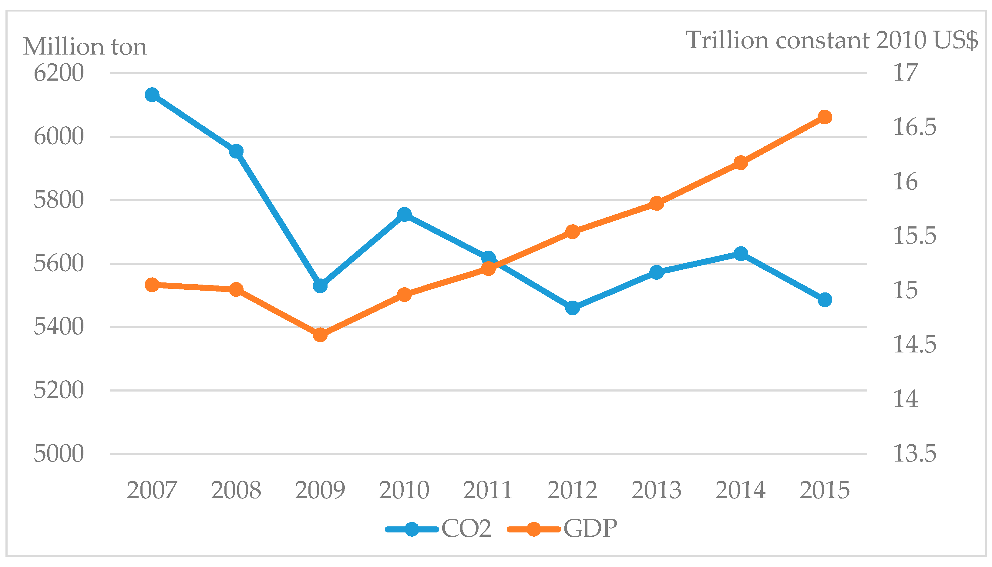
At the 2015 World Climate Conference held in Paris, 196 parties (including 195 separate countries and the entire European Union) came to an agreement on the steps needed to limit global temperature rises to no more than 2 degrees Centigrade. According to previous studies published by the Intergovernmental Panel on Climate Change (IPCC) [16,17], CO2 emissions have historically always increased in line with improvements in the global economy. However, the United States is currently experiencing negative growth in CO2 emissions, while the country’s GDP per capita has continued to grow since 2007. Based on the BP Statistical Review of World Energy 2016 [10,18,19,20], US carbon emissions increased year-on-year before 2007. Then, between 2007 and 2015, US carbon emissions decreased from 6132.4 to 5485.7 Mt per annum, as shown in Figure 1. Accordingly, the US provides a good example for other countries around the world on how to decrease carbon emissions without holding back economic progress. The purpose of this paper is also to reveal the major factors affecting CO2 emissions and thus give other countries useful information to help them formulate effective energy-saving and carbon emission-reduction policies.
After a strong drop from 2007 to 2015, the carbon emissions in 2015 had declined in the US by a full 10%, compared to the 2007 carbon emission levels. However, the country’s gross domestic product (GDP) did not fall. Rather, the GDP continued to show a significant increase, from 15,055.4 billion constant 2010 US$ in 2007, up to 16,597.4 billion constant 2010 US$ in 2015. These figures represent an annual average growth rate of close to 1.25%. Accordingly, the US provides a good example for other countries around the world of how to decrease carbon emissions without holding back economic progress. Simultaneously, the driving force behind this phenomenon is worthy of concentrated investigation. The relevant information would be referential and useful for Asian countries in terms of providing the experience related to reducing carbon emissions while still increasing GDP.
2. Literature Review
In previous studies, Birgit Friedl et al. [21] used the Environmental Kuznets Curve (EKC) to explore the relationship between economic growth and carbon dioxide emissions in Austria over the period from 1960 to 1999. The study concluded that there is a cubic relationship between GDP per capita and CO2 emissions. Lojo Menyah et al. [22] found a unidirectional causality without feedback from US nuclear energy consumption to CO2 emissions from 1960 to 2007, by using the Granger causality test. However, in reality there is no causality from renewable energy consumption to carbon dioxide emissions. Susan Sunlia Sharma [23] confirmed for the global panel that GDP per capita and per capita total primary energy consumption are the determinants of CO2 emissions. Moreover, trade openness, per capita electric power consumption and urbanization all have a negative impact on CO2 emissions. Eyou Dogan et al. [24] adopted an Environmental Kuznets Curve model to study the effects on CO2 emissions of renewable energy consumption, non-renewable sources, real income and trade openness in the European Union. This study, which covered the years from 1980 to 2012, indicated that a bidirectional causality running between renewable energy and CO2 emissions exists, while a unidirectional causality was found from real income to CO2 emissions, from CO2 emissions to non-renewable energy sources, and from trade openness to CO2 emissions. Kais Saidi et al. [25] found a bidirectional causality between labor and capital, and between CO2 emissions and capital, as well as a unidirectional causality from labor to CO2 emissions. This study employed the dynamic panel method and covered nine developed countries over the period from 1990 to 2013. According to the experimental results of Zakaria et al. [26], renewable energy has a negative effect on CO2 emissions. In addition, renewable energy is an effective alternative to conventional fossil fuels in the long term. Wang Q analyzed the importance of renewable energy on reducing carbon emissions in China [27,28,29] and elaborated upon the energy environment now facing China [28,30,31,32,33,34]. Some studies have taken the US as an example. These studies explore the carbon emissions from different sources, such as land-use change [35,36,37,38], farm operations [39], agriculture and forestry [40], and international trade [41]. In addition, other studies have analyzed the impact of energy consumption and income on carbon emissions [42].
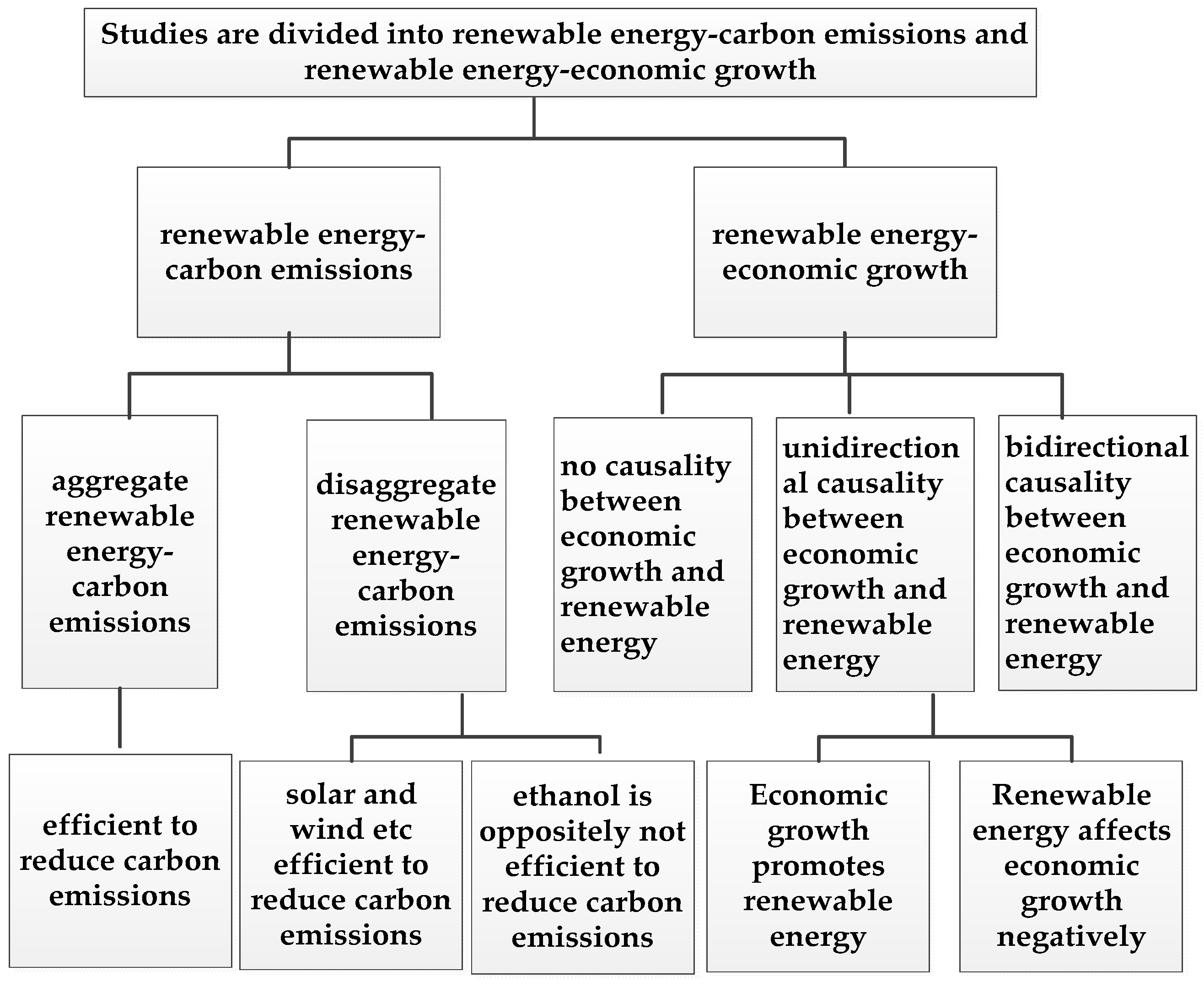
Furthermore, we use the meta-analytic method [43,44,45] to enrich the review of literature related to renewable energy. The studies related to renewable energy are mostly classified into two categories. The first category explores the relationship between renewable energy and carbon emissions. The second category explores the relationship between renewable energy and economic growth. These renewable energy-carbon emissions studies are mostly focused on two aspects, namely, (1) aggregate renewable energy-carbon emissions studies which employ total renewable energy as a whole, and (2) disaggregate renewable energy-carbon emissions studies which concentrate on specific types of renewable energy (namely solar, wind, ethanol, etc.). According to Table 1, we can conclude that the aggregate amount of renewable energy is efficient to reduce carbon emissions. We also find that disaggregate renewable energy has different effects on carbon emissions. Specifically, the use of solar, wind and other forms of renewable energy is an efficient means by which to reduce carbon emissions. However, conversely, some types of renewable energy (e.g., ethanol) are not efficient means by which to reduce carbon emissions. These energy types are shown in detail in Figure 2. According to both Table 2 and Figure 2, we can see three categories with which exhibit no causality, bidirectional causality and unidirectional causality between economic growth and renewable energy. In addition, there are two categories exhibiting unidirectional causality between economic growth and renewable energy, including examples in which economic growth promotes renewable energy, and in which renewable energy negatively affects economic growth. These examples are shown in detail in Figure 2.
A number of studies have already attempted to examine the determinants of CO2 emissions. Most of these studies used different econometric methods, including bivariate and multivariate models, and time series and panel data analyses, as methods to find the determinants of CO2 emissions when given the usage of a set of variables. Nevertheless, no definitive conclusions have yet been made about which factors could have a significant impact on reducing CO2 emissions, especially as regards the function of renewable energy. The above research methods are well worth learning and provide a reference for us. Great differences still exist in the study of the interaction and causality between renewable energy and carbon emissions among foreign scholars. This paper aims to establish the determinants of CO2 emission reductions, as well as the relationship between renewable energy and carbon emissions in the US, between 2007 and 2015.
3. Materials and Methods
3.1. Model Equation
In this paper, time-series data are used to explore changes in the levels of CO2 emissions. We use Equation (1) and take into account the variables that substantially affect carbon emissions, in order to calculate carbon dioxide emissions [58,59,60,61,62]. Our method is based on the vector auto-regression (VAR) model proposed by Burbidge [63], as follows:
where represents carbon dioxide emissions at time t; represents the renewable energy consumption (the sum of hydroelectricity and other renewable energy); represents economic growth; represents primary energy consumption; represents natural gas consumption, represents the error term. As reported in previous studies, economic growth and primary energy consumption have a positive impact on CO2 emissions. In such cases, the signs of , are both expected to be positive. In addition, using renewable energy and natural gas can actually reduce carbon emissions to a certain extent, so the signs of , should be negative in the long-run.
Time-series data analysis based on the VAR model includes six aspects [64]: (1) unit root test, (2) cointegration test, (3) optimal lag order test, (4) Granger causality test, (5) variance decomposition, (6) impulse responses analysis. The vector auto-regression model (VAR) is used to predict and analyze the dynamic impact of random disturbance on the system. The core idea of modeling is to construct a model by taking each exogenous variable as a function of the lagged values of all endogenous variables. Before modeling, we need to test the stationary nature of variables and then, in turn, perform the cointegration test and causality test. In general, the unit root test and cointegration test in the time series are usually required and necessary before building the VAR model in which statistical inferences are conducted [65]. Usually, the root test is employed to conduct a stationary analysis of all variable quantities before the cointegration analysis [60]. We also conducted the unit root test to ensure the stationary property, subsequent to the cointegration test [66], which is to measure whether there is the long-run equilibrium relationship between total carbon dioxide emissions and the effect of each factor or not. Once all the variables are stationary and the long-run equilibrium relationship between total carbon dioxide emissions and the effect of each factor is established, it is prepared to the Granger causality test and to build the VAR model.
In this study, we conducted an augmented Dickey–Fuller (ADF) unit root test and a Johansen cointegration test. The augmented Dickey–Fuller (ADF) unit root test is the most commonly used unit root test and has non-distribution traits, even asymptotically [67] The advantage of the ADF unit root test and the endogenous break unit root tests is that they omit the possibility of a unit root with a break [68], subsequent to the running of the Johansen cointegration test. A common practice to test for cointegration is, in fact, the Johansen cointegration test, which has the maximum likelihood estimator for a cointegrated system with Gaussian errors [69]. This test is applied to check for multivariate cointegrating relationships, which in turn meets the requirements of this study [70,71]. This is why we selected the Johansen cointegration test to analyze the long-run equilibrium relationship between total carbon dioxide emissions and the effect of each factor.
3.1.1. Cointegration Analysis
To investigate the long-term equilibrium relationship between renewable energy consumption, economic growth, primary energy consumption, natural gas consumption and carbon dioxide emissions, our paper employs the VAR model first proposed by C.A. Sims [72]. The unconstrained error correction regression of Equation (1) is represented as follows [73]:
where represents the first order difference of variables; is the intercept term, and parameter n represents the lag lengths. The proper lag length is selected based on the Akaike information criterion (AIC) or final prediction error (FPE). What’s more, the null hypothesis () of no long-term equilibrium relationship should be contrasted with another hypothesis (). If the calculated statistics are between the upper and lower critical values, then the test result is uncertain. If the calculated statistic exceeds the upper critical value, this means that the null hypothesis is rejected, while if the calculated statistic is lower than the lower bound, it means that there is no cointegration relationship between these variables.
3.1.2. Granger Causality Test
The existence of a cointegration relationship shows that a causal relationship exists between variables. However, the direction of that causality is not clear. For that reason, the Granger causality test is applied to investigate the short and long term dynamic causal relationship between variables. Suppose that the variables are non-stationary and that a cointegration relationship exists between the variables. Then, Equation (3) develops a vector error correction model, in order to investigate the Granger causality between variables, as follows:
Before the cointegration test, the optimal lag order aims to select the appropriate lag order, using the AIC or SC minimum value to choose the lag period. A different lag period will lead to significant differences in the estimated results of the model [74].
3.2. Data Source
The observations and data of the US during the 1990–2015 period were obtained from the BP Statistical Review of World Energy (2016) [18]. Carbon emissions were calculated using the total amount of carbon dioxide emissions (measured in million tons). Renewable energy consumption (including hydroelectricity and other renewable energy such as solar, wind, biomass and geothermal), and primary energy consumption were also measured in terms of equivalent million tons of oil. Natural gas consumption figures exclude those of natural gas converted to liquid fuels, but they include gas derivatives of coal, as well as natural gas consumed in gas-to-liquid forms. Primary energy consumption comprises commercially-traded fuels and includes modern renewable energy types used to generate electricity. The actual per capita GDP figures collected from the World Bank were calculated using a constant $2010. Table 3 summarizes the descriptive statistics of the variables estimated in Equation (1). The descriptive statistics of the variable growth rates are shown in Table 4.
4. Analysis Results
4.1. Augmented Dickey-Fuller Unit Root Test
The VAR method is not suitable for the cointegration test until the variables have actually passed the unit root test. Therefore, the unit root test must be conducted before using the VAR method. In order to improve the reliability of the unit root test for each variable, our paper uses the Dickey-Fuller generalized least squares (DF-GLS) method, with a constant and time series. Our test results show that the logarithmic forms of all variables, except and , are stable after taking the second difference; all other variables are stationary when taking the first difference, as shown in Table 5. In addition, the VAR method is applicable for a cointegration test only when the time trend remains steady.
4.2. Johansen Cointegration Test
Based on the stationarity test, we can further perform the Johansen cointegration test represented in Table 6, thereby laying the foundations for the next Granger causality test. This test shows that at least three co-integrating relationships exist between the variables at the 5% confidence level. In conclusion, the calculated results indicate that at least three cointegrating relationships exist between carbon dioxide emissions and renewable energy consumption, economic growth, primary energy consumption, and natural gas consumption.
4.3. Optimal Lag Order
Another important aspect of the VAR estimation model is the choice of the lag period. It is very important for the VAR model to select the appropriate lag order, because different lag periods can lead to different results. Here, we choose the optimal lag period according to the AIC or SC minimum criterion. In consideration of the influence of lag length on significance tests, it is necessary to select the appropriate lag order when using the VAR model. The optimal lag order is determined by the following system-wide method: Akaike information criterion (AIC), Final Prediction Error (FPE) criterion, Hannan-Quinn (HQ) criterion, Schwarz information criterion (SIC) and likelihood ratio (LR). Our experimental results show that the optimal lag length is 3 (Table 7).
We then used the Ordinary Least Squares (OLS) method to calculate the coefficients of Equation (1). As shown in the linear regression (Table 8), the coefficients of Ln and Lnare positive. This result is in accordance with previous literature. The coefficient of Ln is negative, thereby implying that the use of renewable energy benefits carbon reduction efforts. Also, the coefficient of Ln is 0.044435, indicating that natural gas consumption will not have a notable influence on carbon emission reductions in the short term.
4.4. The Granger Causality Results
The results of our Granger causality analysis are displayed in Table 9. We employed p-values to test the causal relationship between two variables. That is to say, the two variables have a causality when their p-values are lower than 0.05 or 0.1; otherwise no causality exists. From the following table, the use of renewable energy and the level of carbon dioxide emissions has a bidirectional relationship, suggesting that these two factors interact with each other in the long term. These findings imply that the construction and maintenance of renewable energy power generation facilities may result in high energy consumption and additional emissions in the short term, but these facilities would do well in terms of reducing carbon emissions in the future. A two-way causal relationship also exists between economic growth and carbon dioxide emissions. This finding indicates that an increase in per capita GDP will lead to an increase in carbon dioxide emissions in the long run. As we all know, carbon emission levels will increase as we use more primary energy sources. As such, a two-way relationship exists between these two factors. In addition, the consumption of natural gas will also influence CO2 emission levels.
4.5. Variance Decomposition
As can be seen from Figure 3, all the roots of the VAR model are in the unit circle and their modules are less than 1, which shows that the VAR model is stable. We can utilize the model to analyze the following variance decomposition and impulse response function on this basis. The stability of the VAR model is the prerequisite for variance decomposition and impulse responses analysis.
Based on several of the above procedures, we built a vector auto-regression model (VAR) for the purpose of analyzing the dynamic effects of different variables on CO2 emissions. Moreover, the variance decomposition method [75] was used to quantitatively study the relationship between the different variables (Table 10). For instance, during Period 10, S.E. is 0.053, which consisted of 68% residual shock from S.E. itself, 5.7% from natural gas consumption, 9.9% from primary energy consumption, 7.8% from the use of renewable energy and 8.2% from economic growth. In a word, primary energy consumption has greatly influenced the level of CO2 emissions, compared to other variables (especially natural gas consumption).
4.6. Impulse Responses Analysis
Finally, the Impulse Responses Function (IRF) method was employed to settle the dispute over which variable contributed most greatly to emissions reductions in the US during the 2007–2015 period. The Impulse Response Function (IRF) is the trajectory of the impact of a standard deviation shock on the current and future values of the endogenous variables. Also, the IRF can accurately describe the dynamic interaction between variables.
Figure 4 is the response of carbon emissions to the emissions themselves. As we can see from Figure 4, there has been no immediate response to the positive impact of a standard deviation of emissions during the current period. In addition, emission levels are in a state of fluctuation at all times in the abovementioned graph. The emission levels decreased rapidly during the first phase, until the minimum value was reached in the second period, when the levels suffered a negative shock from themselves. Subsequently, CO2 levels maintained an upward trend, right up to the time the maximum level was reached in Period 4, where the levels have a positive influence on themselves. Overall, emission levels have been in a state of fluctuation, but the amplitude of that fluctuation is getting smaller and smaller, thereby indicating that carbon emissions will gradually become stable at some point in the future.
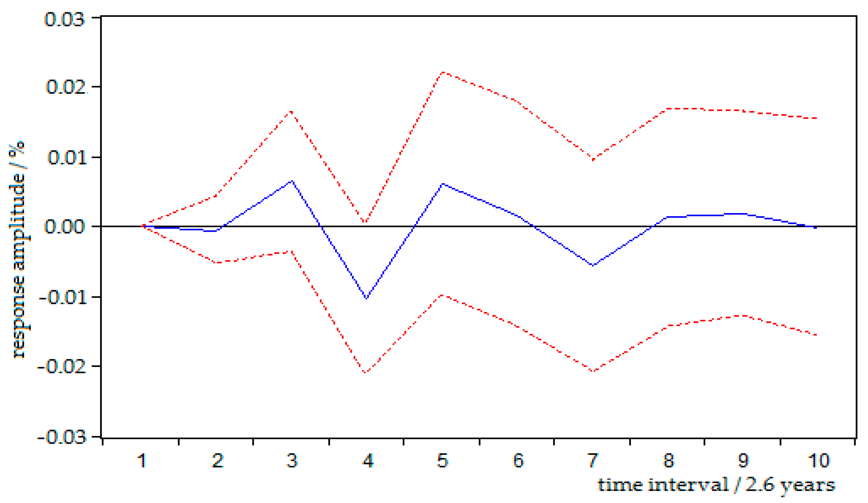
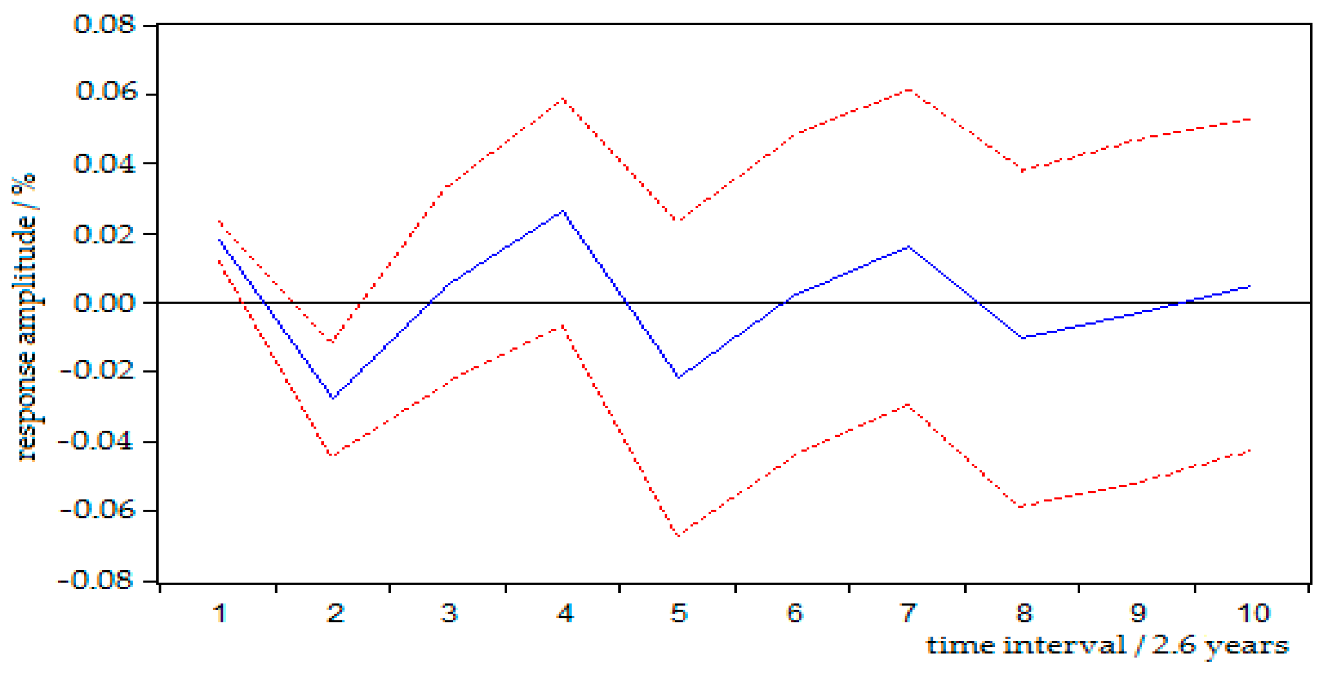
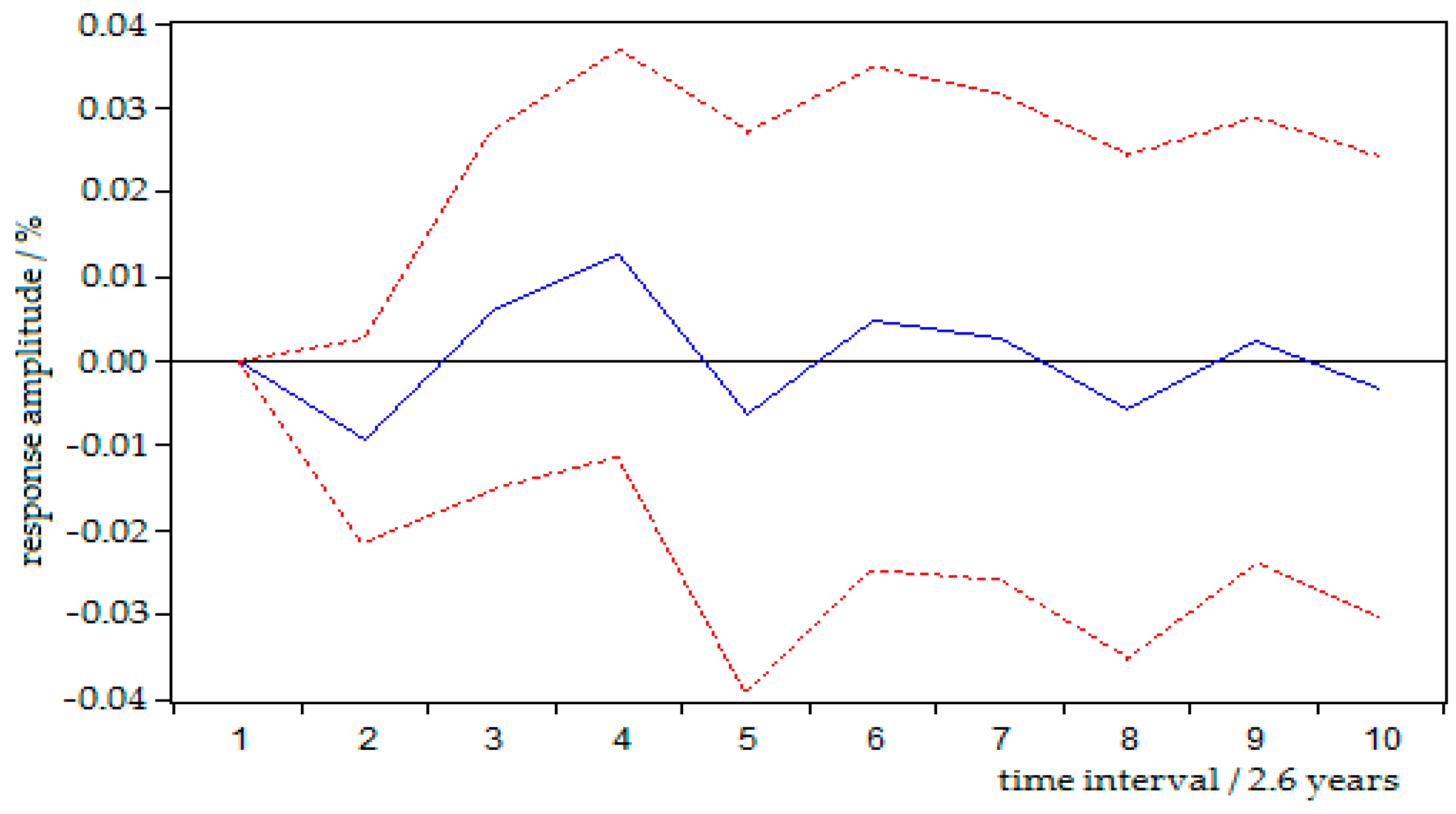
Figure 5, Figure 6, Figure 7 and Figure 8 show the IRF of the annual changes in emissions from renewable energy consumption, natural gas consumption, primary energy consumption and economic growth. As shown in these figures, the horizontal axis represents the number of lag periods of the impact, and the default value is 10 (unit = 2.6 years). The vertical axis represents changes in carbon emissions (unit of measure: %). Furthermore, there are three lines in the graphs. The solid line represents the IRF, while the dashed lines represent the deviation of the positive and negative two times standard deviation.
From Figure 5, we see that a positive, ongoing shock from the use of renewable energy will reduce emission levels in the beginning, before returning to zero in the second period. From Phases 3 to 9, the volatility of emission levels is relatively large. Respectively, emission levels reached their lowest point (−0.028927) in the fourth period and reached their highest point (0.017969) in the ninth period. In the ninth period, the consumption of renewable energy was given a significant positive concussion, resulting in the emission levels falling rapidly, until reaching −0.012521 in the tenth period. Therefore, we believe that emission reductions in the United States during the 2007–2015 period was most likely caused by the extensive use of renewable energy sources.
Figure 6 depicts the impact of natural gas consumption on emissions. As shown in the figure, the level of emissions will decrease in line with the positive shock of natural gas consumption in the early stage. Then, levels gradually rose, due to another positive impact in Period 2, before reaching the highest point (0.12729) during the fourth phrase. After that, emission levels show a downward trend when subjected to the negative impact of natural gas use. From the fifth to the eighth phase, emission levels continue to fluctuate as a result of alternative positive and negative shocks. The results suggest that the consumption of natural gas has so far contributed to a reduction in emissions, but not significantly.
As we can see in Figure 7, emission levels maintained their upward trend in the beginning and then began to decline after suffering the negative impact of primary energy consumption in Period 3. In addition, with the alternation of positive and negative shocks, the emission levels change continuously until the ninth period before reaching a stable state, at which time primary energy consumption has a positive impact on emissions. We can see from these findings that primary energy consumption will increase carbon emission levels.
As we can clearly see in Figure 8,
emission levels have no immediate response to the negative impact of economic growth, at least in the very beginning. When affected by a positive impact from economic growth, carbon emission levels began to increase, until they peaked at 0.006451 in Period 3. After that, emission levels appear to diminish rapidly and down to their minimum in Period 4, with a corresponding negative economic growth. As time went on, the level of
emissions gradually stabilized in the eighth to the tenth phase, but still remained positive. In this case, we can say that economic growth also led to an increase in carbon emissions.
Hence, we can draw a conclusion from the IRF results that the use of renewable energy was the main cause of emissions reductions in the US during the 2007–2015 period. The use of natural gas does not have a significant impact on emissions reductions, despite the fact that the use of natural gas will mitigate carbon dioxide emissions to a certain extent, according to the IRF. In addition, primary energy consumption was the biggest single factor leading to the increase in emissions during the period from 1990–2015, followed by economic growth.
5. Conclusions and Policy Implications
In view of the above findings, we can mainly draw the following conclusions: The Johansen cointegration test results confirmed that, whether in the short term or long term, renewable energy consumption, primary energy consumption, economic development and natural gas consumption all have a certain degree of equilibrium relationship with CO2 emissions in the US. According to the Granger causality test results, we can see that a bidirectional causality exists between CO2 emissions and four other variables. We can also say that CO2 emission levels and the variables covered in this paper affected each other over the past two or three decades in the United States. In addition, a bidirectional causality also existed between the four variables (except for a unidirectional causality from economic growth to renewable energy) in the 1990–2015 period covered by our study.
Variance decomposition results showed that primary energy consumption is the single biggest factor affecting CO2 emissions of the four given variables, in addition to the impact of carbon dioxide itself. Primary energy consumption had a positive and notable influence on CO2 emissions throughout the entire experimental interval. Economic growth and renewable energy consumption are the second and third most influential factors that influence CO2 emission levels. Alternatively, natural gas consumption is the least influential factor and made the smallest contribution to changes in CO2 emission levels, compared to the other variables. From the perspective of the Impulse Responses Function (IRF) results, renewable energy consumption played an important role in lowering US CO2 emissions in Period 10. On the other hand, natural gas consumption resulted in a decrease in CO2 emission levels during the early stage but led to a positive upward trend in the end. Therefore, we believe that the US CO2 emissions reductions did not result from natural gas consumption during the 2007–2015 period. In brief, an increase in CO2 emission levels mainly depended on the given level of economic development, as well as the degree of primary energy consumption. Conversely, the decrease in CO2 emissions was primarily due to the increase in renewable energy consumption.
The above conclusions can provide useful information for policy makers when devising carbon reduction policies. Specifically:
(1) It is necessary to raise the proportion of renewable energy in the overall energy structure as much as possible. For example, biogas, solar energy, biomass energy and other renewable energies all release very little carbon dioxide during use. Since there is a unidirectional causality from economic growth to renewable energy without feedback, any increase in the use of renewable energy will not do any harm to the national economy. In other words, the economy will continue to grow, even in the case of reducing carbon emissions.
(2) Of course, technological innovation should be encouraged, in order to develop new energy and clean energy forms which release less or even no carbon dioxide. Hydroelectric power, onshore wind power and other technologies should continue to be promoted for the purpose of optimizing the energy structure. Furthermore, natural gas exploitation should be accelerated, and the proportion of natural gas consumption (rather than traditional fossil fuels) should be gradually increased, in order to reduce the impact on the environment. The government should also strengthen relevant publicity and education, in order to improve people’s awareness of environmental protection and energy-saving issues. At the same time, the government should encourage the public to use recyclable materials in daily life, instead of disposable and non-recyclable articles. Establishing and perfecting the relevant legal mechanisms as a means of ensuring that energy-saving and carbon emission-reduction policies are implemented smoothly will also be an indispensable step.
(3) Improving energy efficiency is another effective measure which can be employed to mitigate carbon emissions, as a positive correlation exists between primary energy consumption and emissions. Industrial enterprises should gradually reduce their dependence on fossil fuels and exercise strict control over their greenhouse gas emissions, so as not to destroy the environment for the sake of manufacturing.
(4) In particular, the low carbon lifestyle should continue to be strongly advocated in the future. For instance, green travel should be vigorously advocated. Green transport initiatives can reduce vehicle exhaust emissions and reduce traffic jams and road congestion. In China, the government must also pay close attention to taking the necessary actions to reduce carbon emission levels [10,28,76,77,78,79]. These conclusions can provide useful information for policy makers (including in China) looking to formulate carbon reduction policies. The proportion of renewable energy in terms of the country’s overall energy structure should be raised as much as possible. In addition, the government should strengthen publicity and education to improve people's awareness of environmental protection. The public should also be encouraged to use recyclable materials instead of disposable articles in daily life. Furthermore, a low carbon lifestyle should be strongly advocated.
Acknowledgments
The current work is supported by “the Fundamental Research Funds for the Central Universities(27R1706019B)” and the Recruitment Talent Fund of China University of Petroleum (Huadong) (05Y16060020). We have received the grants in support of our research work. The funds we have received for covering the costs to publish in open access.
Author Contributions
Rongrong Li conceived and designed the experiments and wrote the paper; Rongrong Li and Min Su performed the experiments, analyzed the data and contributed reagents/materials/analysis tools. Min Su selected the data. All authors read and approved the final manuscript.
Conflicts of Interest
The authors declare no conflict of interest.
References
- O’connor, R.E.; Bord, R.J.; Fisher, A. Risk perceptions, general environmental beliefs, and willingness to address climate change. Risk Anal. 1999, 19, 461–471. [Google Scholar] [CrossRef]
- Pielke, R.; Prins, G.; Rayner, S.; Sarewitz, D. Climate change 2007: Lifting the taboo on adaptation. Nature 2007, 445, 597–598. [Google Scholar] [CrossRef] [PubMed]
- Hotchkiss, E.; Hall, R., Jr.; Sponseller, R.; Butman, D.; Klaminder, J.; Laudon, H.; Rosvall, M.; Karlsson, J. Sources of and processes controlling CO2 emissions change with the size of streams and rivers. Nat. Geosci. 2015, 8, 696–699. [Google Scholar] [CrossRef]
- Menyah, K.; Wolde-Rufael, Y. CO2 emissions, nuclear energy, renewable energy and economic growth in the US. Energy Policy 2010, 38, 2911–2915. [Google Scholar] [CrossRef]
- Adamantiades, A.; Kessides, I. Nuclear power for sustainable development: Current status and future prospects. Energy Policy 2009, 37, 5149–5166. [Google Scholar] [CrossRef]
- DeCanio, S.J. The political economy of global carbon emissions reductions. Ecol. Econ. 2009, 68, 915–924. [Google Scholar] [CrossRef]
- Reddy, B.S.; Assenza, G.B. The great climate debate. Energy Policy 2009, 37, 2997–3008. [Google Scholar] [CrossRef]
- Vitousek, P.M.; Mooney, H.A.; Lubchenco, J.; Melillo, J.M. Human domination of Earth’s ecosystems. Science 1997, 277, 494–499. [Google Scholar] [CrossRef]
- Hansen, J.; Sato, M. Regional climate change and national responsibilities. Environ. Res. Lett. 2016, 11, 034009. [Google Scholar] [CrossRef]
- Wang, Q.; Li, R. Journey to burning half of global coal: Trajectory and drivers of China׳s coal use. Renew. Sustain. Energy Rev. 2016, 58, 341–346. [Google Scholar] [CrossRef]
- Wang, Q.; Li, R. Drivers for energy consumption: A comparative analysis of China and India. Renew. Sustain. Energy Rev. 2016, 62, 954–962. [Google Scholar] [CrossRef]
- Wang, Q.; Li, R. Natural gas from shale formation: A research profile. Renew. Sustain. Energy Rev. 2016, 57, 1–6. [Google Scholar] [CrossRef]
- Wang, Q.; Chen, X.; Jha, A.N.; Rogers, H. Natural gas from shale formation–the evolution, evidences and challenges of shale gas revolution in United States. Renew. Sustain. Energy Rev. 2014, 30, 1–28. [Google Scholar] [CrossRef]
- Wang, Q.; Li, R. Research status of shale gas: A review. Renew. Sustain. Energy Rev 2017, 74, 715–720. [Google Scholar] [CrossRef]
- Hughes, J.D. Energy: A reality check on the shale revolution. Nature 2013, 494, 307–308. [Google Scholar] [CrossRef] [PubMed]
- IPCC. Contribution of Working Group III to the Fourth Assessment Report of the Intergovernmental Panel on Climate Change Cambridge; Climate Change 2007; Cambridge University Press: London, UK, 2007. [Google Scholar]
- O’Neill, B.C.; Oppenheimer, M.; Warren, R.; Hallegatte, S.; Kopp, R.E.; Pörtner, H.O.; Scholes, R.; Birkmann, J.; Foden, W.; Licker, R. IPCC reasons for concern regarding climate change risks. Nat. Climate Chang. 2017, 7, 28–37. [Google Scholar] [CrossRef]
- BP Statistical Review of World Energy. Available online: http://www.bp.com/en/global/corporate/energy-economics/statistical-review-of-world-energy.html (accessed on 10 April 2017).
- Sakata, M.; Phan, H.G.; Mitsunobu, S. Variations in atmospheric concentrations and isotopic compositions of gaseous and particulate boron in Shizuoka City, Japan. Atmos. Environ. 2017, 148, 376–381. [Google Scholar] [CrossRef]
- Lee, J.S.; Won, D.I.; Jung, W.J.; Son, H.J.; Pac, C.; Kang, S.O. Widely controllable syngas production by a dye-sensitized TiO2 hybrid system with ReI and CoIII catalysts under visible-light irradiation. Angew. Chem. Int. Ed. 2017, 56, 976–980. [Google Scholar] [CrossRef] [PubMed]
- Friedl, B.; Getzner, M. Determinants of CO2 emissions in a small open economy. Ecol. Econ. 2003, 45, 133–148. [Google Scholar] [CrossRef]
- Menyah, K.; Wolde-Rufael, Y. Energy consumption, pollutant emissions and economic growth in South Africa. Energy Econom. 2010, 32, 1374–1382. [Google Scholar] [CrossRef]
- Sharma, S.S. Determinants of carbon dioxide emissions: Empirical evidence from 69 countries. Appl. Energy 2011, 88, 376–382. [Google Scholar] [CrossRef]
- Dogan, E.; Seker, F. Determinants of CO2 emissions in the European Union: The role of renewable and non-renewable energy. Renew. Energy 2016, 94, 429–439. [Google Scholar] [CrossRef]
- Saidi, K.; Mbarek, M.B. Nuclear energy, renewable energy, CO2 emissions, and economic growth for nine developed countries: Evidence from panel Granger causality tests. Prog. Nucl. Energy 2016, 88, 364–374. [Google Scholar] [CrossRef]
- Zoundi, Z. CO2 emissions, renewable energy and the Environmental Kuznets Curve, a panel cointegration approach. Renew. Sustain. Energy Rev. 2016. [Google Scholar] [CrossRef]
- Wang, Q.; Li, R. Impact of cheaper oil on economic system and climate change: A SWOT analysis. Renew. Sustain. Energy Rev. 2016, 54, 925–931. [Google Scholar] [CrossRef]
- Wang, Q.; Chen, X. Energy policies for managing China’s carbon emission. Renew. Sustain. Energy Rev. 2015, 50, 470–479. [Google Scholar] [CrossRef]
- Wang, Q. Effective policies for renewable energy—The example of China’s wind power—Lessons for China’s photovoltaic power. Renew. Sustain. Energy Rev. 2010, 14, 702–712. [Google Scholar] [CrossRef]
- Wang, Q. Cheaper oil challenge and opportunity for climate change. Environ. Sci. Technol. 2015, 49, 1997–1998. [Google Scholar] [CrossRef] [PubMed]
- Wang, Q.; Li, R. Cheaper oil: A turning point in Paris climate talk? Renew. Sustain. Energy Rev. 2015, 52, 1186–1192. [Google Scholar] [CrossRef]
- Wang, Q. Nuclear safety lies in greater transparency. Nature 2013, 494, 403. [Google Scholar] [CrossRef] [PubMed]
- Wang, Q.; Li, R. Sino-Venezuelan oil-for-loan deal—The Chinese strategic gamble? Renew. Sustain. Energy Rev. 2016, 64, 817–822. [Google Scholar] [CrossRef]
- Wang, Q. China needs workers more than academics. Nature 2013, 499, 381. [Google Scholar] [CrossRef] [PubMed]
- Searchinger, T.; Heimlich, R.; Houghton, R.A.; Dong, F.; Elobeid, A.; Fabiosa, J.; Tokgoz, S.; Hayes, D.; Yu, T.-H. Use of US croplands for biofuels increases greenhouse gases through emissions from land-use change. Science 2008, 319, 1238–1240. [Google Scholar] [CrossRef] [PubMed]
- Houghton, R.; Hackler, J.; Lawrence, K. The US carbon budget: Contributions from land-use change. Science 1999, 285, 574–578. [Google Scholar] [CrossRef] [PubMed]
- Fargione, J.; Hill, J.; Tilman, D.; Polasky, S.; Hawthorne, P. Land clearing and the biofuel carbon debt. Science 2008, 319, 1235–1238. [Google Scholar] [CrossRef] [PubMed]
- Hertel, T.W.; Golub, A.A.; Jones, A.D.; O’Hare, M.; Plevin, R.J.; Kammen, D.M. Effects of US maize ethanol on global land use and greenhouse gas emissions: Estimating market-mediated responses. BioScience 2010, 60, 223–231. [Google Scholar] [CrossRef]
- Lal, R. Carbon emission from farm operations. Environ. Int. 2004, 30, 981–990. [Google Scholar] [CrossRef] [PubMed]
- McCarl, B.A.; Schneider, U.A. Greenhouse gas mitigation in US agriculture and forestry. Science 2001, 294, 2481–2482. [Google Scholar] [CrossRef] [PubMed]
- Weber, C.L.; Matthews, H.S. Embodied environmental emissions in US international trade, 1997−2004. Environ. Sci. Technol. 2007, 41, 4875–4881. [Google Scholar] [PubMed]
- Soytas, U.; Sari, R.; Ewing, B.T. Energy consumption, income, and carbon emissions in the United States. Ecol. Econ. 2007, 62, 482–489. [Google Scholar] [CrossRef]
- Menegaki, A.N.; Tiwari, A.K. The index of sustainable economic welfare in the energy-growth nexus for American countries. Ecol. Indic. 2017, 72, 494–509. [Google Scholar] [CrossRef]
- Armitage, C.J.; Conner, M. Efficacy of the theory of planned behaviour: A meta-analytic review. Br. J. Soc. Psychol. 2001, 40, 471–499. [Google Scholar] [CrossRef] [PubMed]
- Martin, D.J.; Garske, J.P.; Davis, M.K. Relation of the therapeutic alliance with outcome and other variables: A meta-analytic review. J. Consult. Clin. Psychol. 2000, 68, 438–450. [Google Scholar] [CrossRef] [PubMed]
- Sims, R. Renewable energy: A response to climate change. Sol. Energy 2004, 76, 9–17. [Google Scholar] [CrossRef]
- Sims, R.E.H.; Rogner, H.H.; Gregory, K. Carbon emission and mitigation cost comparisons between fossil fuel, nuclear and renewable energy resources for electricity generation. Energy Policy 2003, 31, 1315–1326. [Google Scholar] [CrossRef]
- Perry, S.; Klemeš, J.; Bulatov, I. Integrating waste and renewable energy to reduce the carbon footprint of locally integrated energy sectors. Energy 2008, 33, 1489–1497. [Google Scholar] [CrossRef]
- De Oliveira, M.E.D.; Vaughan, B.E.; Rykiel, E.J. Ethanol as fuel: Energy, carbon dioxide balances, and ecological footprint. BioScience 2005, 55, 593–602. [Google Scholar] [CrossRef]
- Vehmas, J.; Luukkanen, J.; Kaivo-oja, J. Linking analyses and environmental Kuznets curves for aggregated material flows in the EU. J. Clean. Prod. 2007, 15, 1662–1673. [Google Scholar] [CrossRef]
- Panwar, N.; Kaushik, S.; Kothari, S. Role of renewable energy sources in environmental protection: A review. Renew. Sustain. Energy Rev. 2011, 15, 1513–1524. [Google Scholar] [CrossRef]
- Sadorsky, P. Renewable energy consumption, CO2 emissions and oil prices in the G7 countries. Energy Econ. 2009, 31, 456–462. [Google Scholar] [CrossRef]
- Bowden, N.; Payne, J.E. Sectoral analysis of the causal relationship between renewable and non-renewable energy consumption and real output in the US. Energy Sources Part B Econ. Plan. Policy 2010, 5, 400–408. [Google Scholar] [CrossRef]
- Apergis, N.; Payne, J.E. Renewable energy consumption and economic growth: Evidence from a panel of OECD countries. Energy Policy 2010, 38, 656–660. [Google Scholar] [CrossRef]
- Menegaki, A.N.; Tsagarakis, K.P. Rich enough to go renewable, but too early to leave fossil energy? Renew. Sustain. Energy Rev. 2015, 41, 1465–1477. [Google Scholar] [CrossRef]
- Marques, A.C.; Fuinhas, J.A.; Menegaki, A.N. Renewable vs non-renewable electricity and the industrial production nexus: Evidence from an ARDL bounds test approach for Greece. Renew. Energy 2016, 96, 645–655. [Google Scholar] [CrossRef]
- Menegaki, A.N.; Ozturk, I. Renewable energy, rents and GDP growth in MENA countries. Energy Sour. Part B: Econ.Plan. Policy 2014. [Google Scholar] [CrossRef]
- Saidi, K.; Mbarek Mbarek, M.B.; Saidi, K. How Effective Are Renewable Energy in Addition of Economic Growth and Curbing CO2 Emissions in the Long Run? A Panel Data Analysis for Four Mediterranean Countries. J. Knowl. Econom. 2016. [Google Scholar] [CrossRef]
- Baek, J. Do nuclear and renewable energy improve the environment? Empirical evidence from the United States. Ecol. Indic. 2016, 66, 352–356. [Google Scholar] [CrossRef]
- Wang, Q.; Li, R.; Jiang, R. Decoupling and Decomposition Analysis of Carbon Emissions from Industry: A Case Study from China. Sustainability 2016, 8, 1059. [Google Scholar] [CrossRef]
- Wang, Q.; Jiang, X.-T.; Li, R. Comparative decoupling analysis of energy-related carbon emission from electric output of electricity sector in Shandong Province, China. Energy 2017, 127, 78–88. [Google Scholar] [CrossRef]
- Wang, Q.; Chen, X. China’s electricity market-oriented reform: From an absolute to a relative monopoly. Energy Policy 2012, 51, 143–148. [Google Scholar] [CrossRef]
- Burbidge, J.; Harrison, A. Testing for the effects of oil-price rises using vector autoregressions. Int. Econ. Rev. 1984, 459–484. [Google Scholar] [CrossRef]
- Wang, Y.; Zhang, Q.; Wang, J. Analysis of influencing factors of oil consumption in China based on VAR model. J. Shenyang Univ. Technol. (Soc. Sci. Ed.) 2017, 10. [Google Scholar] [CrossRef]
- Toda, H.Y.; Yamamoto, T. Statistical inference in vector autoregressions with possibly integrated processes. J. Econ. 1995, 66, 225–250. [Google Scholar] [CrossRef]
- Granger, C.W. Some recent development in a concept of causality. J. Econ. 1988, 39, 199–211. [Google Scholar] [CrossRef]
- MacKinnon, J.G. Numerical distribution functions for unit root and cointegration tests. J. Appl. Econ. 1996, 601–618. [Google Scholar] [CrossRef]
- Lee, J.; Strazicich, M.C. Minimum lagrange multiplier unit root test with two structural breaks. Rev. Econ. Stat. 2003, 85, 1082–1089. [Google Scholar] [CrossRef]
- Crowder, W.J.; Hamed, A. A cointegration test for oil futures market efficiency. J. Futures Mark. 1993, 13, 933–941. [Google Scholar] [CrossRef]
- Maddala, G.S.; Kim, I.-M. Unit Roots, Cointegration, and Structural Change; Cambridge University Press: Cambridge, UK, 1998. [Google Scholar]
- Christopoulos, D.K.; Tsionas, E.G. Financial development and economic growth: Evidence from panel unit root and cointegration tests. J. Dev. Econ. 2004, 73, 55–74. [Google Scholar] [CrossRef]
- Pesaran, M.H.; Shin, Y. An autoregressive distributed-lag modelling approach to cointegration analysis. Econ. Soc. Monogr. 1998, 31, 371–413. [Google Scholar]
- Narayan, P.K. The saving and investment nexus for China: Evidence from cointegration tests. Appl. Econ. 2005, 37, 1979–1990. [Google Scholar] [CrossRef]
- Guo, J. Dynamic Analysis of the Energy Economy and Study on the Energy Efficiency. Ph.D. Thesis, Tianjin University, Tianjin, China, June 2007. [Google Scholar]
- Campbell, J.Y.; Ammer, J. What moves the stock and bond markets? A variance decomposition for long-term asset returns. J. Financ. 1993, 48, 3–37. [Google Scholar] [CrossRef]
- Wang, Q. China has the capacity to lead in carbon trading. Nature 2013, 493, 273. [Google Scholar] [CrossRef] [PubMed]
- Wang, Q. China should aim for a total cap on emissions. Nature 2014, 512, 115. [Google Scholar] [CrossRef] [PubMed]
- Wang, Q. China’s citizens must act to save their environment. Nature 2013, 497, 159. [Google Scholar] [CrossRef] [PubMed]
- Wang, Q.; Li, R.; Hua, L. Toward decoupling: Growing GDP without growing carbon emissions. Environ. Sci. Technol. 2016, 50, 11435. [Google Scholar] [CrossRef] [PubMed]
Figure 1.
The trend of CO2 emissions and GDP of US from 2007 to 2015.

Figure 2.
A fresh meta-analytic categorization of renewable energy-carbon emissions and renewable energy-economic growth literature.
Figure 2.
A fresh meta-analytic categorization of renewable energy-carbon emissions and renewable energy-economic growth literature.

Figure 3.
Stability test of VAR model.
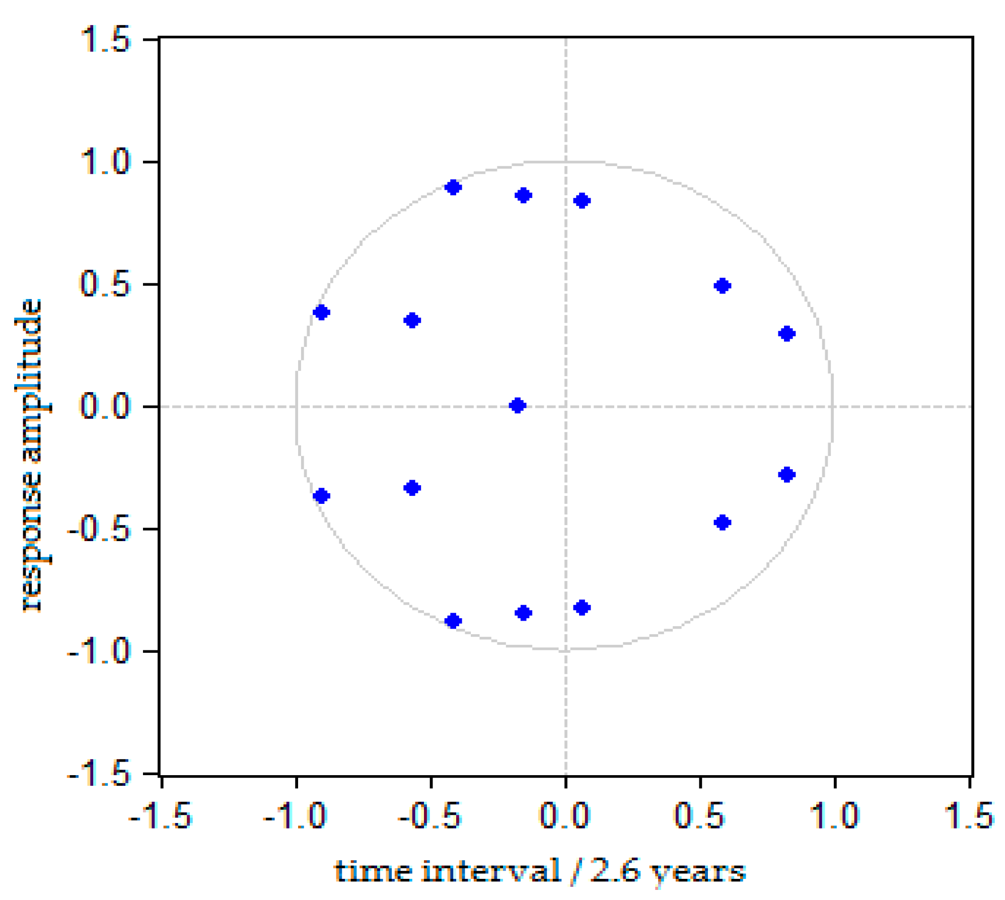
Figure 4.
Response of to .

Figure 5.
Response of to RE.
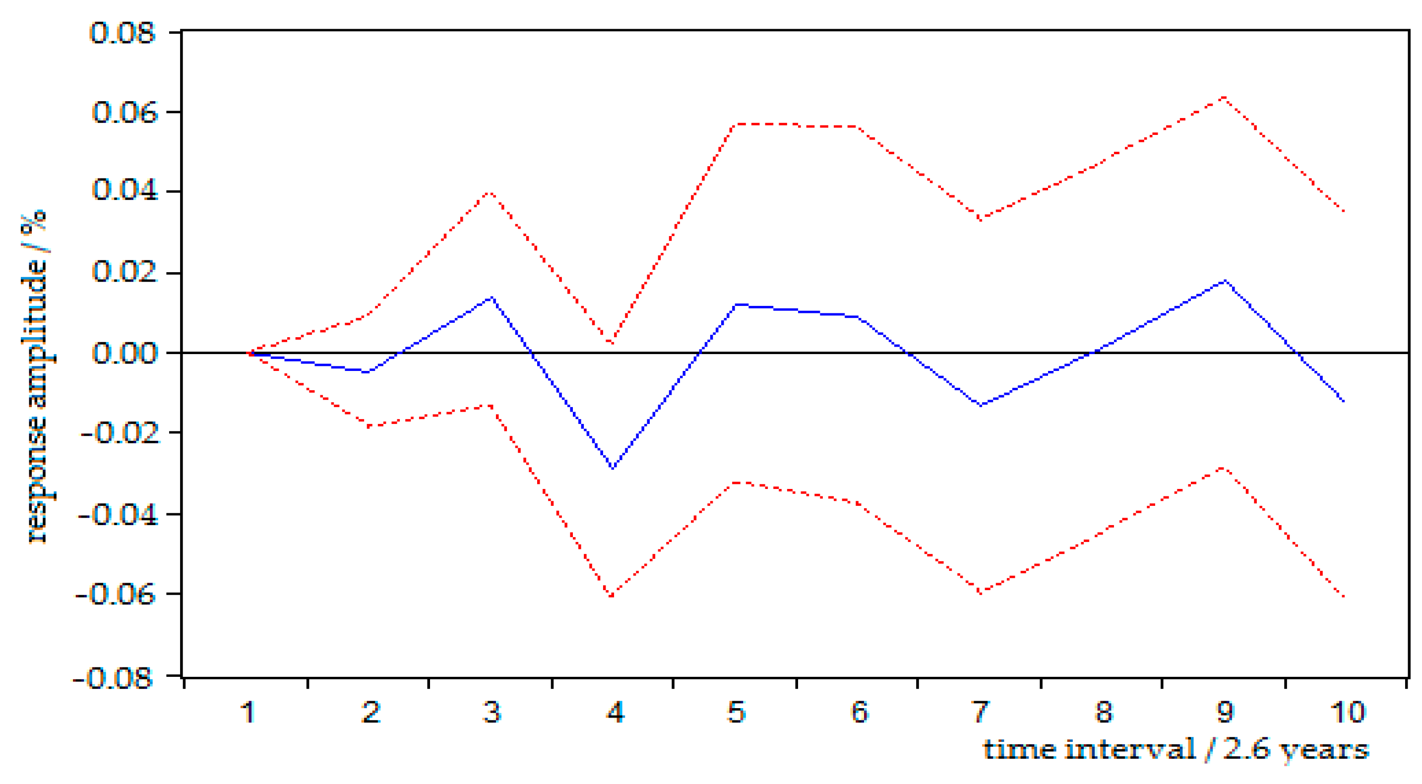
Figure 6.
Response of to NG.

Figure 7.
Response of to PE.
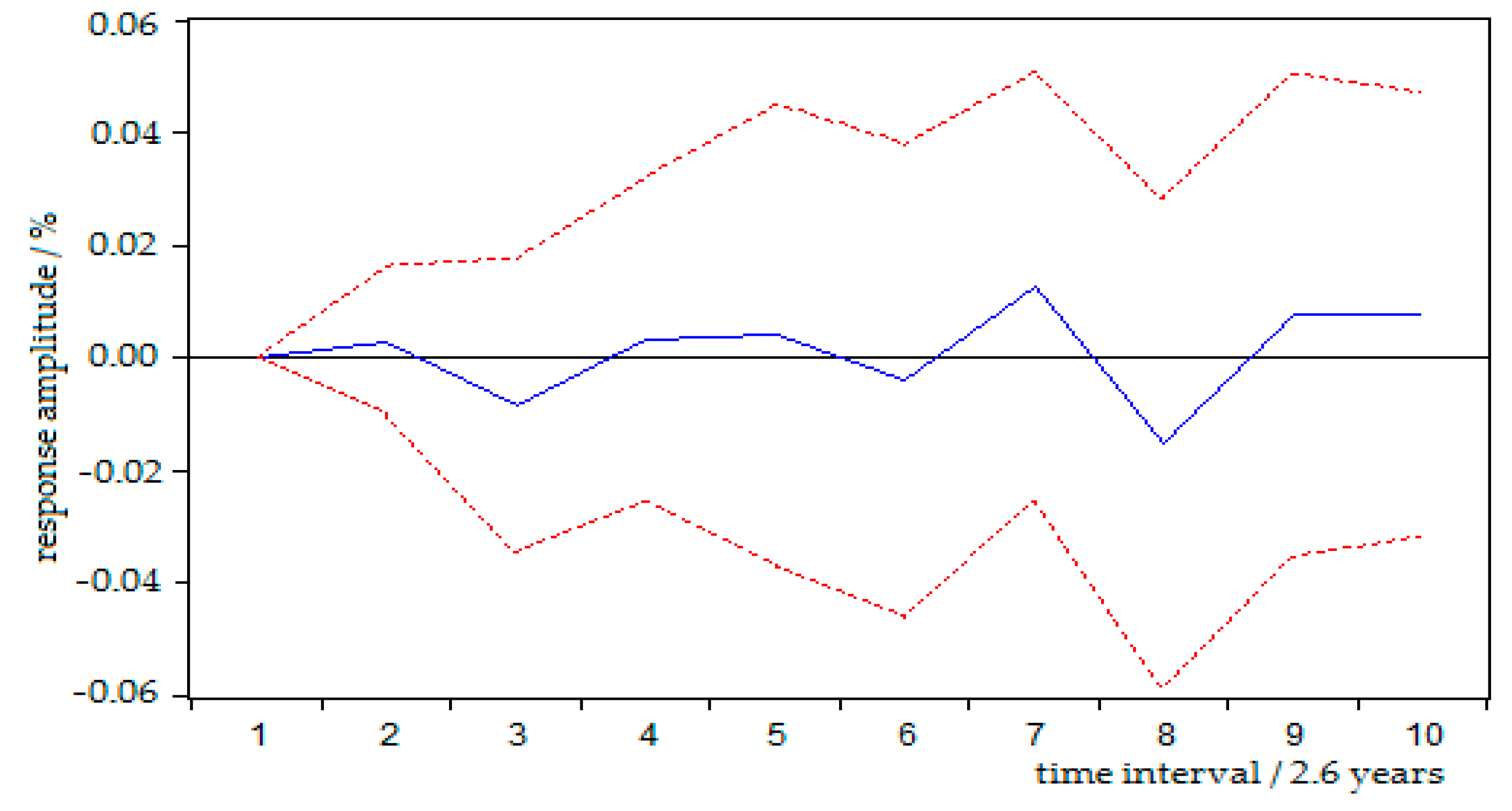
Figure 8.
Response of to Y.

Table 1.
The renewable energy-carbon emissions studies.
| Study | Data-Span | Method | Country | Variables Used | Major Findings |
|---|---|---|---|---|---|
| Renewable energy: a response to climate change [46] | 2010–2020 | Scenario analysis | The world | CO2 emissions, the cost and amount of renewable energy | CO2 reduction potential is from renewable energy |
| Carbon emission and mitigation cost comparisons between fossil fuel nuclear and renewable energy resources for electricity generation [47] | 2010 and 2020 | Scenario analysis | Annex I and non-Annex I countries | Energy source; generating costs; emissions; cost of C reduction; reduction potential to 2010; reduction potential to 2020 | Greater use of renewable energy is efficient to reduce CO2 emissions |
| Integrating waste and renewable energy to reduce the carbon footprint of locally integrated energy sectors [48] | 2008 | Total site targeting methodology | UK | Carbon footprint; combined heat and power generation; process stream supply temperature, etc. | Integrate renewables into the energy source mix and consequently reduce carbon emissions |
| Ethanol as fuel: energy, carbon dioxide balances, and ecological footprint [49] | 2001 | STELLA model | Brazil and US | Ethanol production; CO2 emissions | Accompanying environmental impacts of use of ethanol outweigh its benefits |
| Plug-in vehicles and renewable energy sources for cost and emission reductions [50] | 2011 | Smart grid model | The world | Renewable energy, mainly wind and solar, CO2 emission from the electricity industry | Renewable energy can reduce emissions from the electricity industry |
| Role of renewable energy sources in environmental protection: a review [51] | 2001, 2010, 2020, 2030, 2040 | Scenario analysis | The world | Main renewable energy sources; CO2 emissions | Renewable energy is an excellent opportunity for the mitigation of greenhouse gas emissions |
| CO2 emissions, nuclear energy, renewable energy and economic growth in the US [4] | 1960–2007 | Granger causality test | US | CO2 emissions; renewable energy | Renewable energy consumption did not help in mitigating CO2 emissions |
Table 2.
The renewable energy-economic growth studies.
| Study | Data-Span | Method | Country | Variables Used | Major Findings |
|---|---|---|---|---|---|
| CO2 emissions, nuclear energy, renewable energy and economic growth in the US [4] | 1960–2007 | Granger causality test | US | Economic growth; renewable energy | Economic growth promotes renewable energy consumption |
| Renewable energy consumption, CO2 emissions and oil prices in the G7 countries [52] | 1980–2005 | Panel cointegration | G7 countries | Renewable energy; income elasticity; CO2; oil prices | Economic growth is an important driver of renewable energy consumption |
| Sectoral analysis of the causal relationship between renewable and non-renewable energy consumption and real output in the US [53] | 1949–2006 | Toda-Yamamoto long-run causality tests | US | GDP; renewable energy | No causality between GDP and renewable energy |
| Renewable energy consumption and economic growth: evidence from a panel of OECD countries [54] | 1985–2005 | cointegration test | OECD countries | Economic growth; renewable energy | Bidirectional causality between renewable energy consumption and economic growth in both the short- and long-run |
| Rich enough to go renewable, but too early to leave fossil energy? [55] | 1990–2010 | Random effect Arellano Bond estimator models | 33 European members | Renewable energy production; GDP per capita | Economic growth causes consecutive rebounds to renewable energy development |
| Renewable vs non-renewable electricity and the industrial production nexus: Evidence from an ARDL bounds test approach for Greece [56] | August. 2004 to February 2014 | Autoregressive Distributed Lag bounds test | Greece | Renewable and non-renewableelectricity; economic growth | In the short-run, fossil sources play the baseload role in electricity production; in the long-run, fossil sources contribute to the development of renewable energy sources |
| Renewable energy, rents and GDP growth in MENA countries [57] | 1997–2009 | Dynamic, fixed effects model | MENA countries | Renewable energy; GDP growth; employment, etc. | Renewable energy affects GDP growth negatively in the long-run |
Table 3.
Descriptive statistics for the variables.
| Variable | Mean | Std. Dev. | Min | Max |
|---|---|---|---|---|
| 5675.5787 | 298.4913 | 5117.4537 | 6132.4197 | |
| 92.0171 | 16.8601 | 66.3806 | 129.1542 | |
| 12,974,847 | 2,415,938 | 9,057,698 | 16,597,445 | |
| 2221.3920 | 120.8930 | 1965.0325 | 2371.8237 | |
| 589.1269 | 52.5359 | 493.9915 | 713.6022 |
Table 4.
Descriptive statistics for the growth rates of variables.
| Variable | Mean | Std. Dev. | Min | Max |
|---|---|---|---|---|
| 1.002747 | 0.024951 | 0.928739 | 1.040659 | |
| 1.022648 | 0.091738 | 0.822833 | 1.201531 | |
| 1.024629 | 0.017075 | 0.972245 | 1.046852 | |
| 1.006129 | 0.020396 | 0.950802 | 1.035899 | |
| 1.015160 | 0.026657 | 0.955867 | 1.064033 |
Table 5.
Results of unit root test.
| Variable | Level | First Difference | Second Difference | |||
|---|---|---|---|---|---|---|
| t-Statistic | Prob. * | t-Statistic | Prob. * | t-Statistic | Prob. * | |
| Ln | −1.841293 | 0.3530 | −1.566869 | 0.4820 | −8.972583 | 0.0000 |
| Ln | −2.308182 | 0.1772 | −1.617599 | 0.4572 | −9.101436 | 0.0000 |
| Ln | −0.545182 | 0.8659 | −5.358222 | 0.0002 | – | – |
| Ln | −0.376888 | 0.8989 | −5.399738 | 0.0002 | – | – |
| Ln | −1.823769 | 0.3609 | −3.177550 | 0.0341 | – | – |
* Indicates Mackinnon (1996) one-side p-values.
Table 6.
Results of cointegration test.
| Hypothesized No. of CE(S) | Eigenvalue | Trace Statistic | 0.05 Critical Value | Prob. ** |
|---|---|---|---|---|
| None * | 0.919073 | 115.7581 | 69.81889 | 0.0000 |
| At most 1 * | 0.742273 | 60.44548 | 47.85613 | 0.0021 |
| At most 2 * | 0.604860 | 30.61668 | 29.79707 | 0.0402 |
| At most 3 | 0.270599 | 10.18937 | 15.49471 | 0.2665 |
| At most 4 | 0.137243 | 3.247687 | 3.841466 | 0.0715 |
* Denotes rejection of the hypothesis at the 0.05 level; ** Mackinnon-Haug-Michelis (1999) p-values. Trace test indicates three cointegrating equation(s) at the 0.05 level.
Table 7.
Lag order selection criteria.
| Lag | LogL | LR | FPE | AIC | SC | HQ |
|---|---|---|---|---|---|---|
| 0 | 235.1871 | NA | 2.07 × 10⁻¹⁶ | −21.92258 | −21.67388 | −21.86860 |
| 1 | 271.2822 | 51.56453 * | 7.82 × 10⁻¹⁷ | −22.97926 | −21.48708 | −22.65542 |
| 2 | 301.7092 | 28.97807 | 7.66 × 10⁻¹⁷ | −23.49611 | −20.76046 | −22.90241 |
| 3 | 357.7041 | 26.66423 | 2.45 × 10⁻¹⁷ * | −26.44801 * | −22.46887 * | −25.58443 * |
* Indicates the lag order selected by the following criterion: LR, likelihood ratio; FPE, Final Prediction Error; AIC, Akaike information criterion; HQ, Hannan-Quinn criterion; SC, Schwarz information criterion.
Table 8.
Results of Ordinary Least Squares (OLS).
| Variable | Coefficient | Std. Error | t-Statistic | Prob |
|---|---|---|---|---|
| Ln | −0.045808 | 0.028137 | −1.628034 | 0.1200 |
| Ln | 0.105815 | 0.163473 | 0.647292 | 0.5252 |
| Ln | 1.127493 | 0.098137 | 11.48901 | 0.0000 |
| Ln | 0.044435 | 0.109412 | 0.406130 | 0.6892 |
| c | −0.002813 | 0.005133 | −0.548125 | 0.5900 |
Table 9.
Granger causality test.
| Dependent Variable | Ln | Ln | Ln | Ln | Ln |
|---|---|---|---|---|---|
| Ln | – | 0.2006 (1.76849) | 0.5638 (0.59287) | 0.5717 (0.57788) | 0.6972 (0.36845) |
| Ln | 0.7432 (0.30210) | – | 0.7497 (0.29297) | 0.6944 (0.37219) | 0.0250 (4.55736) |
| Ln | 0.6227 (0.48718) | 0.3317 (1.17851) | – | 0.2786 (1.37918) | 0.4816 (0.76297) |
| Ln | 0.7634 (0.27424) | 0.7132 (0.34444) | 0.9208 (0.08290) | – | 0.5750 (0.57069) |
| Ln | 0.6465 (0.44763) | 0.2785 (1.37351) | 0.8012 (0.22459) | 0.2513 (1.49263) | – |
Prob-values is in the first line and F-Statistic is in ( ).
Table 10.
Variance decomposition of CO2.
| Period | S.E. | Ng | pe | re | y | |
|---|---|---|---|---|---|---|
| 1 | 0.025133 | 100.0000 | 0.000000 | 0.000000 | 0.000000 | 0.000000 |
| 2 | 0.039725 | 89.43859 | 1.449627 | 5.034572 | 2.776565 | 1.300651 |
| 3 | 0.042684 | 78.92087 | 1.571097 | 11.28675 | 2.435458 | 5.785829 |
| 4 | 0.047363 | 71.65297 | 4.225139 | 9.598777 | 6.036759 | 8.486356 |
| 5 | 0.049212 | 70.77241 | 5.112457 | 9.706330 | 6.536472 | 7.872331 |
| 6 | 0.049934 | 69.66817 | 4.990904 | 10.29472 | 6.665203 | 8.380999 |
| 7 | 0.051677 | 69.45335 | 5.462661 | 9.636757 | 7.444748 | 8.002480 |
| 8 | 0.052093 | 68.96800 | 5.500810 | 10.03408 | 7.357998 | 8.139121 |
| 9 | 0.052631 | 68.50340 | 5.542318 | 10.00261 | 7.612963 | 8.338717 |
| 10 | 0.053133 | 68.47273 | 5.693212 | 9.876224 | 7.771473 | 8.186361 |
© 2017 by the authors. Licensee MDPI, Basel, Switzerland. This article is an open access article distributed under the terms and conditions of the Creative Commons Attribution (CC BY) license (http://creativecommons.org/licenses/by/4.0/).
Share and Cite
MDPI and ACS Style
Li, R.; Su, M. The Role of Natural Gas and Renewable Energy in Curbing Carbon Emission: Case Study of the United States. Sustainability 2017, 9, 600. https://doi.org/10.3390/su9040600
AMA Style
Li R, Su M. The Role of Natural Gas and Renewable Energy in Curbing Carbon Emission: Case Study of the United States. Sustainability. 2017; 9(4):600. https://doi.org/10.3390/su9040600
Chicago/Turabian StyleLi, Rongrong, and Min Su. 2017. "The Role of Natural Gas and Renewable Energy in Curbing Carbon Emission: Case Study of the United States" Sustainability 9, no. 4: 600. https://doi.org/10.3390/su9040600
Note that from the first issue of 2016, this journal uses article numbers instead of page numbers. See further details here.