The Impact of Beijing Subway’s New Fare Policy on Riders’ Attitude, Travel Pattern and Demand

Abstract

On 28 December 2014, the Beijing subway’s fare policy was changed from “Two Yuan” per trip to the era of Logging Ticket Price, charging users by travel mileage. This paper aims at investigating the effects of Beijing subway’s new fare policy on the riders’ attitude, travel pattern and demand. A survey analysis was conducted to identify the effects of the new fare policy for Beijing subway on riders’ satisfaction degree and travel pattern associated with the potential influencing factors using Hierarchical Tree-based Regression (HTBR) models. The model results show that income, travel distance and month of travel have significant impacts on the subway riders’ satisfaction degree, while trip purpose, car ownership and travel frequency significantly influence the riders’ stated travel pattern. Overall, the degree of satisfaction could not be effectively recovered within five months after the new fare policy, but the negative public attitude did not depress the subway demand continuously. Based on the further time sequence analyses of the passenger flow volume data for two years, it is concluded that the new policy made the ridership decrease sharply in the first month but gradually came back to the previous level four months later, and then the passenger flow volume kept steady again. The findings in this study indicate that the new fare policy realized the purpose of lowering the government’s financial pressure but did not reduce the subway ridership in a long term perspective.

1. Introduction

In China, rail transit has played an important role in economic vitality and urban sustainable development of the large cities with high population density. As a city’s backbone system, urban rail transportation can satisfy the travel demands of the low income residents and commuters, which assists in creating a better urban environment [1]. Especially, urban rail transit should provide a high level of services in order to shift travelers away from private cars and reduce road traffic congestion [2]. Among the factors that influence the service quality of urban rail transit, fare is the most indispensable and fundamental one [3]. Understanding the relationship between passenger satisfaction trend and fare change will benefit decision makers in developing appropriate fare policies.

In the conventional urban transit industry, a fare increment is typically expected to increase revenue in response to actual or forecasted increase in operating costs, while such an increase usually yields ridership loss [3]. Additionally, many factors were identified which influence transit demand such as fare, car ownership, service quality and so on [4]. After a wide range of factors was examined, it was found that fare has the most significant impact on transit demand [3]. Transit agencies from time to time evaluate feasibility of changes in fares and fare structures in response to transit market demand [5]. Nir and Yoram developed a travel-behavior model for the transit system in the city of Haifa, Israel. The model results show that metro fare reduction was a significant factor for attracting transit users [6]. Similarly, in developed countries, fare policies are also critical measures to regulate and adjust the level of transit ridership, which have been applied by Transport for London, Atlanta Rapid Transit, the transit organization in LA and other metropolitan transit agencies [7,8].

On the other hand, increasing fare of public transit leads to not only the reduction of transit ridership, but also the decrease in the degree of satisfaction of transit passenger. In the field of transportation, researchers are increasingly recognizing the importance of passenger satisfaction [9]. In general, satisfaction is seen as the main drive of consumer loyalty [10]. Customer loyalty is regarded as a prime determinant of firm’s long-term financial performance and is considered a major source of competitive advantage [11]. Customer satisfaction in public transit can be defined as the overall level of attainment of a customer’s expectations, measured as the percentage of the customer expectations met by the transit service [12]. In other studies based on the Theory of Planned Behavior (TPB), customer satisfaction has been widely identified as the most important determinant of favorable behavioral intentions [13,14,15].

Many researchers have conducted studies to identify the significant factors influencing passenger satisfaction or the relationship between the service quality and passenger satisfaction, such as [16,17,18]. Few studies were performed to examine the passenger satisfaction associated with a new transit fare policy implemented. This type of study will help to better understand the impact of the new fare policy, and the research on the degree of satisfaction with the policy will give the transit agency feedback to further improve the service quality.

In fact, it is difficult to accurately predict the relationship between ridership and fare change rate, which is a core issue for making a new fare policy. For example, in New York City, before the fare increase in 2003, the agency did not have any experience with either the direct ridership effects of price change or the shift of customers if the fare increases at different rates [19]. As expected, the effects of the price change on transit demand have attracted major attention in previous studies [20,21,22]. It is worth noting that there are distinctive travel characteristics and cultures among different cities. The influence of fare change on the ridership may display diverse patterns among these cities.

In Beijing, the capital of China, its subway agency implemented a new fare policy on 28 December in 2014, adopting a mileage-based pricing policy to take place of the flat fee policy, which provides a valuable opportunity to investigate the impact of Beijing subway fare change on the riders’ satisfaction and transit demand. Subsequently, we conducted a stated preference (SP) survey on the passengers at three subway stations. The survey data were then examined to understand the riders’ satisfaction and travel behavior. Specifically, the method of Hierarchical Tree-based Regression (HTBR) was used to analyze the survey data. The model results show the significant factors that affect the satisfaction degree of passengers on the new fare policy, and passengers’ travel pattern change after the fare policy implemented. In addition, to evaluate the impacts that the new fare policy has on the passenger demand, we used Beijing subway historic passenger flow volume for empirical assessment. A time series analysis was developed, and the ADF test was used to analyze the Beijing subway passenger flow volume.

2. Background

Beijing is the capital of the People’s Republic of China, and one of the most populous cities in the world. As of the 2015 census bureau population estimate, the population was 21,705,000 [23]. 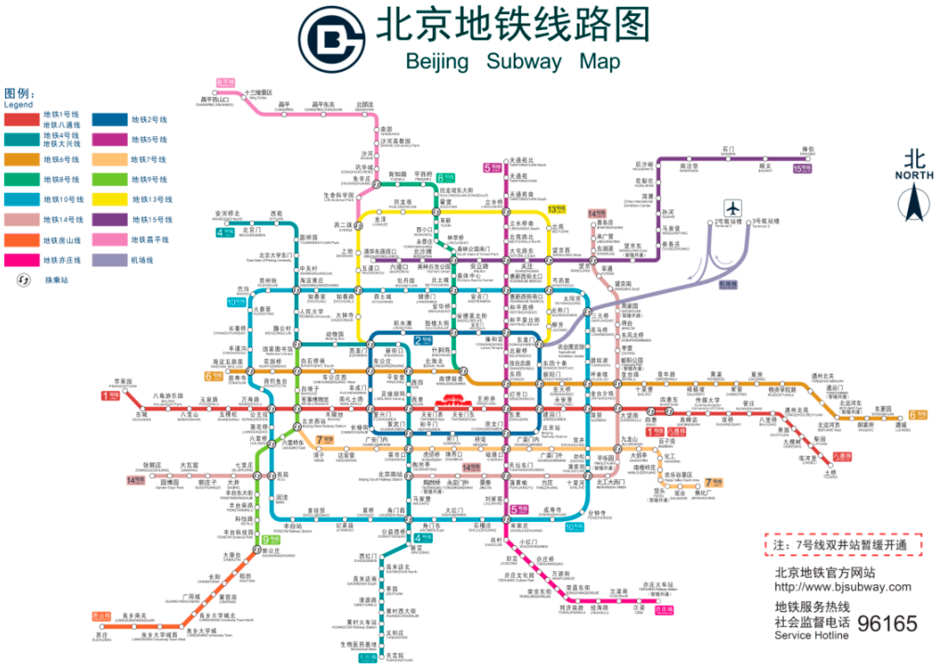Due to the high density of urban development and limited developable land in China, many city governments have chosen public transit as their preferred transportation system to facilitate urbanization and growth [24]. The Beijing public transit system provides an effective travel mode for residents to achieve their various trip purposes; it is approaching its capacity though. The Beijing subway system has a rapid transit network that serves the urban and suburban areas of the city. The network has 18 lines, 334 stations, and 554 km (344 mi) of track in operation [25]. It is the largest subway system in the world by both railway mileage and passenger volume. The Beijing subway route and station map is shown in Figure 1. The subway is the world’s busiest system in annual ridership, with 3.41 billion trips delivered in 2014, averaging 9,278,600 per day, and ridership reaching 11,559,500 in a peak day [25].

Given such a large system, the fare structure was simple in the past: a flat fare of 2 RMB entitled a ticket holder to ride on any or all of the routes in the system with one exception. The route of the Capital Airport Line charges 25 RMB. The fare is the lowest among the subway systems in China. However, based on the long-term plan of Beijing subway, estimated system expansion investment will rise to 297.8 billion RMB by 2020 [26]. The fare revenue of Beijing subway system is not adequate to cover its operating cost, not to mention construction cost of the necessary system expansion. In recent years, the government subsides on public transport in Beijing increase year over year. The bus and rail transit agency in Beijing received the subsidy of 20 billion RMB from governments in 2013 [27]. The subsidy is expected to increase in order to pay for the system expansion and annual maintenance of the system [28]. Meanwhile, due to huge number of transit users and the transit fare lower than its market value, ridership on Beijing subway system becomes increasingly large. The stations and trains are heavily crowded during rush hours, reaching 8 persons per m². The massive numbers of subway riders have caused subway stations to be overcrowded, which creates considerable negative externalities including noise pollution, subway user safety concern, and psychological problems such as commuting stress [29,30,31,32]. Overcrowd mitigation countermeasures have been applied to 40 stations during peak hours; for example, riders are required to wait outside the station to ensure that stations perform at an acceptable level of service [29].

On 28 December 2014, a recent fare change has been implemented in Beijing subway system. Then, the policy of “Two Yuan” fare, which the Beijing subway agency had carried out for the last seven years, officially ended. The agency starts the era of Logging Ticket Price [33], which charges users by travel mileage (The detail information is shown in

Table 1. Detail information of the new subway fare policy.

Mileage (km)	Fare (RMB)
<6	3
6–12	4
12–22	5
22–32	6
>32	Add 1 RMB for extra 1 km

Discount: If spend more than 100 RMB, then the extra part has 80% discount; if spend more than 150 RMB, then the extra part has 50% discount.

). The motivations of the fare policy change are twofold: the first is to reduce the government’s heavy fiscal burden on the urban rail subsides by increasing fare revenue; and the second is to balance the saturated ridership and network capacity because the excessive ridership have led to a public safety concern.

Based on the Beijing case, some studies have been carried out to predict the impact of the fare change on ridership. It was estimated that Beijing subway system ridership would decrease by 30% after the new fare policy was in effect and, consequently, alleviate the safety risks of the crowded subway system, especially in morning and evening peak hours [28]. However, other researchers have different estimate that the new fare policy would not have a significant impact on the ridership because most of the subway riders were composed of the committed or transit dependent subway users [34].

According to the transit ridership statistics on the historical transit fare reform in Beijing, a fare increase had a significant impact on the ridership. For instance, the fare increase that occurred in 1996 and 2000 resulted in the substantial decrease of ridership [35]. Specifically, the fare increase from ¥0.5 to ¥2 in 1996 made the annual ridership drop by 20.4%, from 55,802 million (1995) to 44,414 million (1996) [36]. After a few years, a fare increase from ¥2 to ¥3 in 2000 made the annual ridership decrease by 12.28% [35]. It can be seen that the impact of fare change on the transit ridership varies by different time periods. Therefore, it is important to evaluate whether the recent fare change in 2014 would realize the purposes of decision makers and better understand the evolution of the transit demand owing to the policy reform.

Additionally, in the field of the transportation pricing policy research, a traditional concern on the pricing policy formulation is user equity, which has been discussed for many decades [37]. Equity refers to the distribution of impacts (benefits and costs) and whether the distribution is fair and appropriate. Two categories of equity are acknowledged: horizontal equity and vertical equity. Horizontal equity focuses on how the passengers equally share public resources and spend travel costs [38]. Vertical equity emphasizes allocating resources among individuals according to different abilities and needs, which is to provide resources to those who need the resources most, such as the low-income and youth [37].

Specific to public transportation pricing policy, many previous studies have addressed the equity issues of flat fares versus distance-based fares. Early studies indicated that flat the flat fare polices are neither efficiency nor equitable [39,40]. Comparing five alternative fare proposals of Alameda-Contra District, the flat fares per ride were found to be least equitable, even when the base fare was lowered [5]. The reason is that lower income riders and younger users more frequently rely on the public transportation services than the higher income riders and elder users. Based on travel pattern analyses, lower income riders are found to travel shorter distances and more often during non-rush hours, and thus poor users are actually subsidizing rich ones [41]. Often, a long term of flat fare policy may directly contribute to the financial deterioration and, consequently, increase fares due to budget shortfalls. Then, public transportation operators would shift the flat fares to other fare structures, such as distance-based fares, such as the Beijing case.

In terms of distance-based fares, the distance-based fares generally benefit low-income and elderly riders [42], and the fares differentiated by distance could reduce inequities and improve transits’ financial performance [41]. However, simply increasing transportation price is often criticized as being regressive (burdening disadvantaged people) [38]. Increasing fares for long-distance transit riders may also result in an increased use of less sustainable modes of transportation, such as private cars. Such a change could contribute to increased greenhouse gas emissions, lower air-quality, more traffic accidents and increased traffic congestion, which displays a potential conflict between polices aimed at promoting equity and those intended to encourage public transportation share ratio [42].

The new fare policy of Beijing Subway has a significant impact on the equity of public transportation. On the one hand, the mileage-based fee policy of Beijing Subway may increase horizontal equity for passengers since it makes the ticket price more accurately reflect costs. On the other hand, the new policy may bring vertical equity issues. However, if there are good supplementary policies, the increased revenues can be used to benefit the disadvantaged people by discounts.

3. Methodology

To investigate the impact of the reform of Beijing subway fare policy on subway users’ satisfaction degree and ridership, both questionnaire survey and operation data analyses are needed. Thus, a SP survey was continuously conducted at the most representative Beijing subway stations for four months in order to uncover whether the public travelers were satisfied with the distance-based fare policy reform, whether their travel patterns were changed accordingly, and how the changes in travelers’ attitude and behavior were associated with the traveler characteristics and trip features. A Hierarchical Tree-based Regression (HTBR) method was applied to analyze the survey data. Additionally, an empirical study based on the actual Beijing subway operation data was utilized to evaluate how the new fare policy had an impact on the passenger volume. The time series analyses with the ADF test method were conducted to identify whether there was an immediate mutation (a quick decrease) in passenger volume before and after the policy implementation, and if the passenger volume was sensitive to the policy in a short term, whether the volume could restore to the previous level as the policy had been implemented for a long term.

3.1. Stated Preference Survey

In order to examine the effects factors, such as travel frequency, travel purpose, travel distance, etc., on passenger travel behavior and perception after the new price policy was implemented, a traffic survey was conducted at three different subway stations: Xizhimen subway station, Beijing west subway station, and Huilongguan subway station. The three subway stations selected in the paper are the most representative ones in Beijing. They all have enormous passenger flow volume due to their important functions. Xizhimen subway station is the largest transfer station in Beijing, connecting three major subway lines of Beijing. Huilongguan subway station is one of the largest commuting subway stations, serving for one of the largest residential areas. Beijing west subway station is a subway station connected with a railway station, and its function is to serve the passengers’ departure and arrival at the largest rail station in Beijing.

At each survey site, 180 randomly-selected travelers effectively answered questionnaires in January, March, April and May 2015. No survey was conducted in February as it is the Spring Festival, during which the travel pattern was dramatically changed (due to holiday season). The data were collected between 7:00 a.m. and 9:00 a.m. at each survey site on weekdays, which can efficiently cover both commuters in peak hour and non-commuting travelers in order to balance the sample sizes of different travel purposes.

In this study, three classes of independent variables potentially influencing the target variables (passengers’ travel pattern change and degree of satisfaction to the new fare policy on Beijing subway system) were investigated, namely, demographics, trip purpose, and trip characteristics. Demographic factors include passengers’ gender, age, education level, occupation, income, and car ownership. Trip purpose is categorized into leisure purpose and work/business purpose. Trip characteristics contain variables of travel distance and travel frequency. The variables and their descriptions are listed in

Table 2. Variables in the survey and descriptive statistics.

Variables		Description and Coding of Input Value	Summary Statistics
Name	Description		N	%
Independent Variables
Gender	Passenger’s gender	1 → female	297	54.91%
		2 → male	243	45.09%
Age	Passenger’s age classification	1 → <20	15	2.82%
		2 → 20–29	280	51.86%
		3 → 30–39	178	32.96%
		4 → 40–49	47	8.70%
		5 → >50	20	3.71%
Education	Passenger’s education level	1 → high school or under	276	51.20%
		2 → bachelor degree	226	42.00%
		3 → master degree or above	38	6.80%
Vocation	Passenger’s vocation classification	1 → civil servant	93	17.23%
		2 → farmer	34	6.37%
		3 → enterprise employees	112	20.84%
		4 → small business owner	45	8.29%
		5 → worker	52	9.76%
		6 → free vocation	47	8.67%
		7 → student	99	18.30%
		8 → others	58	10.54%
Income	Passenger’s income level (per month)	1 → <1500 RMB	188	34.81%
		2 → 1500–5000 RMB	135	25.00%
		3 → 5000–10,000 RMB	150	27.78%
		4 → >10,000 RMB	67	12.41%
Purpose	Passenger’s travel purpose	1 → leisure purpose	303	56.10%
		2 → work/business purpose	237	43.90%
Frequency	Passenger’s travel frequency level (per week)	1 → <3	84	15.60%
		2 → 3–4	194	35.90%
		3 → 5–6	75	13.90%
		4 → 7–8	32	5.90%
		5→ >8	155	28.70%
Distance	Passenger’s average travel distance	1 → <5 station	97	18.00%
		2 → 6–10 station	257	47.60%
		3 → >10 station	186	34.40%
Car ownership	Passenger’s car ownership situation	1 → own	416	76.90%
		2 → not own	124	23.10%
Target Variables
Degree of satisfaction	Degree of satisfaction of passengers about the new policy	1 → very dissatisfied	43	7.90%
		2 → dissatisfied	232	42.90%
		3 → just so-so	165	30.50%
		4 → satisfied	70	12.90%
		5 → very satisfied	30	5.50%
Travel pattern change	Passenger’s travel pattern change level after the new policy situation	1 → almost not change	168	31.10%
		2 → a little change	357	66.00%
		3 → most change	15	2.82%

.

Statistical analyses were performed to examine relationships between different groups of passengers and their travel behavior. Particularly, a Hierarchical Tree-based Regression (HTBR) model was developed to identify subgroups of target variables whose members share common characteristics associated with the variables.

3.2. The Hierarchical Tree-Based Regression Method for Survey Data Analyses

Hierarchical Tree-based Regression (HTBR) was first used in the 1960s in the medical and the social sciences. In recent years, the tree-based algorithm has been gradually used in the analysis of transportation studies for analyzing the traffic accident rates and injury severity problems [43,44,45], investigating the travel behavior and transport mode choice [46,47] and identifying the interaction of different transportation characteristics [48].

In contrast to parametric linear regression, HTBR facilitates a piecewise constant approximation to the underlying regression function. Such an approximation can be made to a high degree of accuracy with enhancement on trees [49]. As a non-parametric tool in nature, HTBR relies on few statistical assumptions and does not require a functional form to be specified.

The HTBR procedure creates a tree-based classification model using the CHAID (Chi-Squared Automatic Interaction), CRT (Classification and Regression Trees), or QUEST (Quick, Unbiased, Efficient, and Statistical Tree) algorithm. Among the three algorithms, both CRT and CHAID techniques can construct regression-type trees (continuous dependent variable), where each (non-terminal) node identifies a split condition, to yield optimum prediction. HTBR is non-parametric method which does not require variables to be selected in advance since it uses a stepwise method to determine optimal splitting rules [49]. Further, HTBR has been proved to be an efficient and explicit interpretable approach to explore the relationship between dependent and independent variables. Specifically, the dependent variables in this paper are the degree of satisfaction (nominal variable) and the travel pattern change (nominal variable), and some independent variables are multi-categorical nominal variables.

The specifications for the hierarchical tree construction include: the maximum tree depth was set as 5 levels; the minimum number of cases for parent nodes was set as 50; and the minimum number of cases for child nodes was set as 25. The significance values for both splitting nodes and merging categories are set as 0.05. In order to select the best tree size, the CHAID algorithm is applied for this research since it allows multi-way splits of a node. The full algorithm of CHAID is as follows:

Step 1. For each predictor in turn, cross-tabulate the categories of the predictor with the categories of the dependent variable and do Steps 2 and 3.

Step 2. Find the pair of categories of the predictor (only considering allowable pairs as determined by the type of the predictor) whose 2 × d sub-table is least significantly different. If this significance does not reach a critical value, merge the two categories, consider this merger as a single compound category, and repeat this step.

Step 3. For each compound category consisting of three or more of the original categories, find the most significant binary split (constrained by the type of the predictor) into which the merger may be resolved. If the significance is beyond a critical value, implement the split and return to Step 2.

Step 4. Calculate the significance (to be discussed later) of each optimally merged predictor, and isolate the most significant one. If this significance is greater than a criterion value, subdivide the data according to the (merged) categories of the chosen predictor.

Step 5. For each partition of the data that has not yet been analyzed, return to Step 1. This step may be modified by excluding from further analysis partitions with a small number of observations.

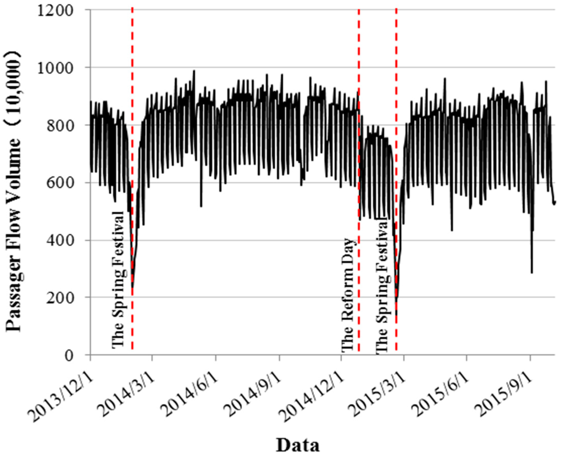
3.3. Time Series Analyses of Passenger Volume

In addition to subway rider survey, an empirical study was further applied to investigate the effects of the Beijing subway fare change on the daily passenger volume. Among different indicators, the passenger flow volume changes before and after the fare policy implementation can directly reveal the impact of the new fare policy. The time series of Beijing subway passenger volume from December 2013 to October 2015 was analyzed. The subway lines on which the volume data were obtained in this study are 1st line, 2nd line, 5th line, 6th line, 7th line, 8th line, 9th line, 10th line, 13th line, 15th line, Batong line, Changping line, Fangshan line, Airport line and Yizhuang line. The volume data can be found in the official website of the Beijing Subway [25].

In the field of time series research, the traditional view that the impact of the current random issues (resulting in the deviation of the trend) generally only has a temporary effect, the long-term variables are driven by a deterministic time trend function, which is called trend stationary. If the time series itself contains unit root (unit root), any random impact will affect its long-term dynamic, resulting in a long-term effect. The ADF test principal is as shown as follows:

Consider a simple general AR(p) progress given by:

$$Y_t=\mu +{\phi }_1{Y}_{t-1}+{\phi }_2{Y}_{t-2}+\dots +{\phi }_p{Y}_{t-p}+{ϵ}_t$$

If this is the process generating the data but an AR(1) model is fitted, say

$$Y_t=\mu +{\phi }_1{Y}_{t-1}+v_t$$

Then,

$$v_t={\phi }_2{Y}_{t-2}+\dots +{\phi }_p{Y}_{t-p}+{ϵ}_t$$

The autocorrelations of $v_t$ and $v_{t-k}$ for $k>1$, will be nonzero because of the presence of the lagged Y terms. Thus, an indication of whether it is appropriate to fit an AR(1) model can be aided by considering the autocorrelations of the residual for the fitted models.

To illustrate how the DF test can be extended to autoregressive processes of order greater than 1, consider the simple AR(2) process below.

$$Y_t=\mu +{\phi }_1{Y}_{t-1}+{\phi }_2{Y}_{t-2}+{ϵ}_t$$

Then, notice that this is the same as:

$$Y_t=\mu +({\phi }_1+{\phi }_2)Y_{t-1}-{\phi }_2(Y_{t-1}-Y_{t-2})+{ϵ}_t$$

Subtracting $Y_{t-1}$ from both sides gives:

$$\Delta Y_t= \mu +\beta Y_{t-1}-{\alpha }_1\Delta Y_{t-1}+{ϵ}_t$$

where the following have been defined:

$$\beta ={\phi }_1+{\phi }_2-1$$

$${\alpha }_1=-{\phi }_2$$

This means that if the appropriate order of the AR process is 2 rather than 1, the term $\Delta Y_{t-1}$ should be added to the regression model. A test of whether there is a unit root can be carried out in the same way as for the DF test, with the test statistics provided by the “t” statistics of the $\beta$ coefficient. If $\beta =0$, then there is a unit root. The same reasoning can be extended for a generic AR(p) model. The following regression should be estimated:

$$\Delta Y_t= \mu +\beta Y_{t-1}-{\displaystyle \sum }_{j=1}^p{\alpha }_j\Delta Y_{t-j}+{ϵ}_t$$

The standard Dickey–Fuller model has been augmented by$\Delta Y_{t-j}$. In this case, the regression model and the “t” test are referred as the ADF test.

In this study, the degree of the ridership change was evaluated and the ADF test (using Eviews-7.2 software) was used to determine if the change is significant after the new fare policy. Three time series patterns were examined as follows:

• Period_Before: 1 May 2014–7 October 2014;
• Period_Between: 1 December 2014–31 January 2015; and
• Period_After: 1 May 2015–7 October 2015.

Accordingly, three hypotheses as below are proposed:

Hypothesis 1.

Time series Period_Before is unstable (time series Total_Part1 has a unit root), which means that the time series before the policy implementation has mutations.

Hypothesis 2.

Time series Period_Between is unstable (time series Total_Part2 has a unit root), which means that the passenger volume has an immediate mutation owning to the policy change.

Hypothesis 3.

Time series Period_After is unstable (Time series Total_Part3 has a unit root), which means that the time series after the policy implementation has mutations.

4. Results

4.1. Descriptive Analysis of Survey Data

4.1.1. Degree of Satisfaction

Figure 2, Figure 3 and Figure 4 display the relationships of the degree of satisfaction on the new fare policy with the statistically significant influencing factors respectively, including month, distance and income. The percentage of respondents who choose “very dissatisfied” (score = 1) and “dissatisfied” (score = 2) decreases gradually month by month. On the contrary, the percentage of respondents choosing “satisfied” (score = 4) and “very satisfied” (score = 5) increases with the increment of month. As the travel distance increased, the degree of satisfaction from respondents becomes lower. For travel distance more than six stations, almost no rider chose “very satisfied” (score = 5). The higher income the respondents have, the higher degree of satisfaction they stated. For the income more than 10,000 RMB group, nearly 30% of respondents chose “very satisfied” (score = 5), while almost no respondent chose “very satisfied” (score = 5) in the income level less than 1500 RMB.

4.1.2. Travel Pattern Change

Figure 5, Figure 6 and Figure 7 displays the relationships of the anticipated travel pattern change due to the new fare policy with the statistically significant influencing factors, respectively, including travel frequency, travel purpose, and car ownership.

The respondents who travel less frequently are more likely to change their travel pattern. For the group with travel frequency less than eight times per week, more than 70% of respondents chose “a little change”, but for the group with travel frequency more than eight times per week, nearly 60% of respondents chose “almost not change”.

The respondents with leisure trip purpose are more likely to change their travel pattern: respectively 5.94% of them chose “almost not change”, 89.11% of them chose “a little change”, and 4.95% of them chose “most change”. On the contrary, the respondents with work/business trip purpose are less likely to change their travel pattern: respectively 62.08% of them chose “almost not change”, 36.71% of them chose “a little change”, and 1.21% of them chose “most change”. The respondents with a car are more inclined to change their travel pattern: 77.42% of them chose “a little change” and 10.48% of them chose “almost not change”. For the respondents who do not have a car, the percentage of choosing “a little change” accounts for 62.74% and t the percentage of choosing “almost not change” is 33.80%.

4.2. Hierarchical Tree-Based Regression Model

4.2.1. HTBR Model #1—Classifying the Degree of Satisfaction

Figure 8 shows the results of the hierarchical tree-based regression model for analyzing the patterns of the riders’ degree of satisfaction on the new Beijing subway fare policy. The final tree structure is comprised of five explanatory variables: income, place, month, distance and purpose.

The first branch of the tree is income, indicating that income plays the most significant role on the degree of satisfaction. It classifies the subway riders into four subgroups based on income: “>10,000 RMB”, “5000–10,000 RMB”, “1500–5000 RMB” and “<1500 RMB”. For the respondents with income more than 10,000 RMB, 26.9% of them are very satisfied with the new fare policy, 19.4% of them are satisfied, the “just so-so” respondents accounts for 34.3%, dissatisfied riders accounts for 16.4%, and 3% responded with “very dissatisfied”. In the group of lower income, the percentage of the respondents with stating “dissatisfied and very dissatisfied” is higher. In the group of income less than 1500 RMB, no respondent chose the “very satisfied” while the respondents who chose “very dissatisfied” and “dissatisfied” accounts for nearly 65%.

The second level of the tree contains three explanatory variables: place, month, and distance. Place and month, respectively, lead to further splits at Nodes 2 and 3; distance divides Node 4 into three terminal nodes (Nodes 9–11). Nodes 5 and 6 show that for income group between 5000 RMB and 10,000 RMB, the respondents’ degree of satisfaction varies by locations. The general trend is that the overall satisfaction degrees in Beijing west subway station and Xizhimen subway station are higher than Huilongguan subway station. In Beijing west and Xizhimen stations, the respondents with “satisfied” are 24 percent for the income group of “1500 RMB–5000 RMB”; in the Huilongguan subway station, the corresponding percentage is 9.3%. For the same income group, 32.3 percent of the respondents chose “very dissatisfied” and “dissatisfied” in Beijing west subway station and Xizhimen subway station; meanwhile, 57.4% of the respondents chose “very dissatisfied” and “dissatisfied” in Huilongguan subway station. The degree of satisfaction seems to differ by month in the income group between 1500 RMB and 5000 RMB: 24.2% of riders responded with “very dissatisfied” in January; and 3.9% in March, April and May. For the income group with less than 1500 RMB, travel distance is a significant factor affecting the degree of satisfaction: more than 80% of the respondents whose average travel distance is more than 10 stations were dissatisfied with the new policy; the same level (dissatisfied) is 37.2% for the respondents whose travel distance is less than six stations.

In the third level of the tree, trip purpose further splits Node 6 into two subgroups. The statistical results indicate that, for the respondents in the Huilongguan subway station, the degree of satisfaction is different among trip purposes: 38.4% of the respondents with leisure trip purpose were dissatisfied with the new policy while 49.2% of the respondents with work/business trip purpose were dissatisfied with the new policy. Location further splits Node 8 into two subgroups, more subway riders in Huilongguan subway station (80% of the respondents) were dissatisfied with the new policy than those riders in Xizhimen and Beijing west subway stations (44.4% of the respondents).

4.2.2. HTBR Model #2—Classifying the Travel Pattern Change

Figure 9 shows the results of the hierarchical tree-based regression model for the relationship between passengers’ travel pattern change and the classified variables. The final tree structure includes three splitting variables: trip purpose, car ownership, and travel frequency.

The first optimal split in Node 0 accords to trip purpose, which classifies the travel pattern change into two subgroups: leisure purpose and work/business purpose. For the group of leisure purpose, the respondents inclined to choose “a little change” (89.11%) after the new fare policy; for the group of work/business purpose, the respondents tended to choose “almost not change” (62.08%).

In the second level of the tree, car ownership further divides Node 1 into two subgroups. Without owning a car, the “almost not change” response accounts for 13.6%, “a little change” response is 81.8%; and “most change” response is 4.5%. On the contrary, for respondents who own a car, no respondent chose “almost not change”, and 93.3% of respondents chose “a little change”.

The final level of the tree shows that travel frequency further splits Node 4 into two subgroups. Terminal Node 5 and Node 6 indicate that the respondents with low travel frequency were less likely to change their travel pattern than those respondents with high travel frequency. For the group of low travel frequency, 96.6% of respondents chose “a little change” and 3.4% of them stated “most change”; for the group of high travel frequency, 83% of respondents chose “a little change” and 17% of them preferred “most change”.

4.3. Time Series Analysis for Travel Demand

4.3.1. General Trend of Passenger Volume

The time series chart of Beijing subway ridership between 1 December 2013 and 7 October 2015 is shown in Figure 10. It was generally stable but during Spring Festival in 2014 and 2015, the passenger flow volume reached its lowest point because a large number of people left Beijing during the holidays. It should be noted that, after 28 December 2014 (the implementation date of the new fare policy), the ridership has a clear downward trend; the trend continued until February 2015; the passenger flow volume began to rebound after the Spring Festival; in May, the passenger flow volume approached the average level of 2014; then the ridership time series become constant. In contrast, for the same period, from December 2013 to the Spring Festival of 2014, the downward trend did not exist.

Further, the time frame from 1 December 2014 to 31 January 2015 was selected for in-depth analysis and its time series chart is shown in Figure 11. It has a certain week periodicity; the ridership on a weekday is significantly higher than the ridership on Saturday or Sunday.

4.3.2. Analyses of the Passenger Flow Volume Declination

Statistical analysis was performed to compare the ridership in different periods, and evaluate the degree of the ridership declined after Beijing subway new fare policy implemented. Table 4 displays the statistics of the passenger flow volume in different periods. There are five periods defined in this analysis:

• Time_period1: 28 December 2014–31 January 2015;
• Time_period2: 1 December 2013–20 January 2014;
• Time_period3: 1 May 2014–1 October 2014;
• Time_period4: 1 May 2015–1 October 2015(without Line 7); and
• Time_period4#: 1 May 2015–1 October 2015 (with Line 7).

Time_period1 starts one month after Beijing subway new fare policy was in effect, which is the basic period as a comparison with other periods. Time_period2 began one year before Beijing subway new fare policy; its duration is 1.5 months. Time_period3 represents the average passenger flow volume in 2014. Time_period4 represents the average passenger flow volume in 2015. In addition, because Beijing subway Line 7 was started on 28 December 2014, the Time_period4# is further examined, taking the ridership of Line 7 into consideration.

In

Table 3. Statistical information of different time period passenger flow volume.

Time Periods	Average Daily Passenger Flow Volume (10,000 Person)	Change Percentages
28 December 2014–31 January 2015	682.4708571
1 December 2013–20 January 2014	757.893	+11.05%
1 May 2014–1 October 2014	820.3445455	+20.20%
1 May 2015–1 October 2015 (without Line 7)	767.2459091	+12.42%
1 May 2015–1 October 2015 (with Line 7)	797.8	+16.90%

, it can be seen that the average daily passenger flow volume is 6,825,000 passengers/day from 28 December 2014 to 31 January 2015, which is the lowest among the five periods. Before the new fare policy, the average daily passenger flow volume from 1 May 2014 to 1 October 2014 is 8,203,000 passengers/day, which is the highest of the five time periods. Time_period2 has the ridership of 7,578,900 passengers/day; Time_period4 has 7,672,500 passengers/day and Time_period5 has 7,978,000 passengers/day. The increasing percentages in comparison with Time_period1 are, respectively, +11.05%, +20.20%, +12.42%, and +16.90%. Passenger flow volume in different periods is shown in Figure 12.

4.3.3. ADF Test

ADF tests were performed to examine the three Hypotheses. Hypothesis 1 is that the time series Period_Before has a unit root, which means that the time series before the policy implementation has mutations. The ADF test result for Hypothesis 1 is shown in

Table 4. Null Hypothesis 1: Period_Before has a unit root.

Lag Length: 14 (Automatic—Based on SIC, Maxlag = 19)
		t-Statistic	Prob.*
Augmented Dickey–Fuller test statistic		−3.678068	0.0047
Test critical values:	1% level	−3.440501
	5% level	−2.865910
	10% level	−2.569155

* MacKinnon (1996) one-sided p-values.

. The t-Statistic is −3.678068, less than critical values at 1%, 5% and 10% significance level, which are −3.440501, −2.865910 and −2.569155, respectively. Meanwhile, its significance coefficient is 0.0047, which is less than 0.05. Therefore, the null hypothesis 1 is rejected indicating that Period_Before does not have a unit root, meaning that the time series before the policy implementation has no significant mutation.

Hypothesis 2 is that the time series Period_Between has a unit root, which means that the passenger volume has an immediate mutation owning to the policy change.

Table 5. Null Hypothesis 2: Period_Between has a unit root.

Lag Length: 7 (Automatic—Based on SIC, Maxlag = 10)
		t-Statistic	Prob.*
Augmented Dickey–Fuller test statistic		−1.620429	0.4654
Test critical values:	1% level	−3.557472
	5% level	−2.916566
	10% level	−2.596116

* MacKinnon (1996) one-sided p-values.

and

Table 6. Null Hypothesis 2*: Period_Between first order difference has a unit root.

Lag Length: 6 (Automatic—Based on SIC, Maxlag = 10)
		t-Statistic	Prob.*
Augmented Dickey–Fuller test statistic		−4.279317	0.0012
Test critical values:	1% level	−3.557472
	5% level	−2.916566
	10% level	−2.596116

* MacKinnon (1996) one-sided p-values.

reveal that the ADF test results for Period_Between that is a non-reposeful time series with integration of order one and the null hypothesis was accepted, which means that the passenger volume has an immediate mutation owing to the policy change.

Hypothesis 3 is that the time series Period_After has a unit root, which means that the time series after the policy implementation has mutations.

Table 7. Null Hypothesis 3: Period_After has a unit root.

Lag Length: 6 (Automatic—Based on SIC, Maxlag = 10)
		t-Statistic	Prob.*
Augmented Dickey–Fuller test statistic		−3.030486	0.0336
Test critical values:	1% level	−3.458719
	5% level	−2.873918
	10% level	−2.573443

* MacKinnon (1996) one-sided p-values.

reveals the ADF test results for Period_After that is a reposeful time series and the null hypothesis was rejected, which means that the time series after the policy implementation has no mutation.

In summary, the passenger flow volume time series from 1 May 2014 to 7 October 2014 maintain overall reposeful; the time series from 1 December 2014 to 31 January 2015 is non-reposeful; and the time series from 1 May 2015 to 7 October 2015 is reposeful. It indicates that the new fare policy indeed has an influence on the ridership right after the policy was implemented; however, the influence gradually disappeared after May 2015. Specifically, after the new fare policy, the ridership decreased substantially for about three months, and then rebounded rapidly back to nearly the previous level.

5. Discussion

During the implementation of a new fare policy for public transportation systems, the passengers’ attitude to the policy should be investigated since it would be anticipated to have an impact on the transit demand [50]. 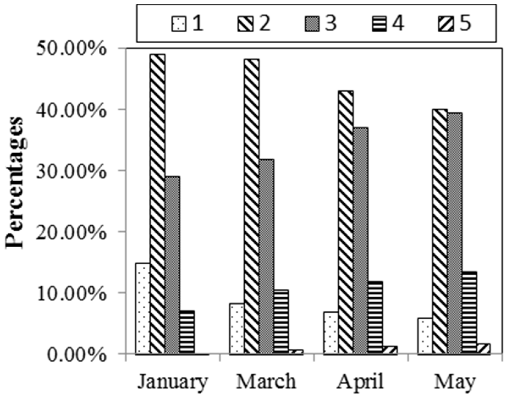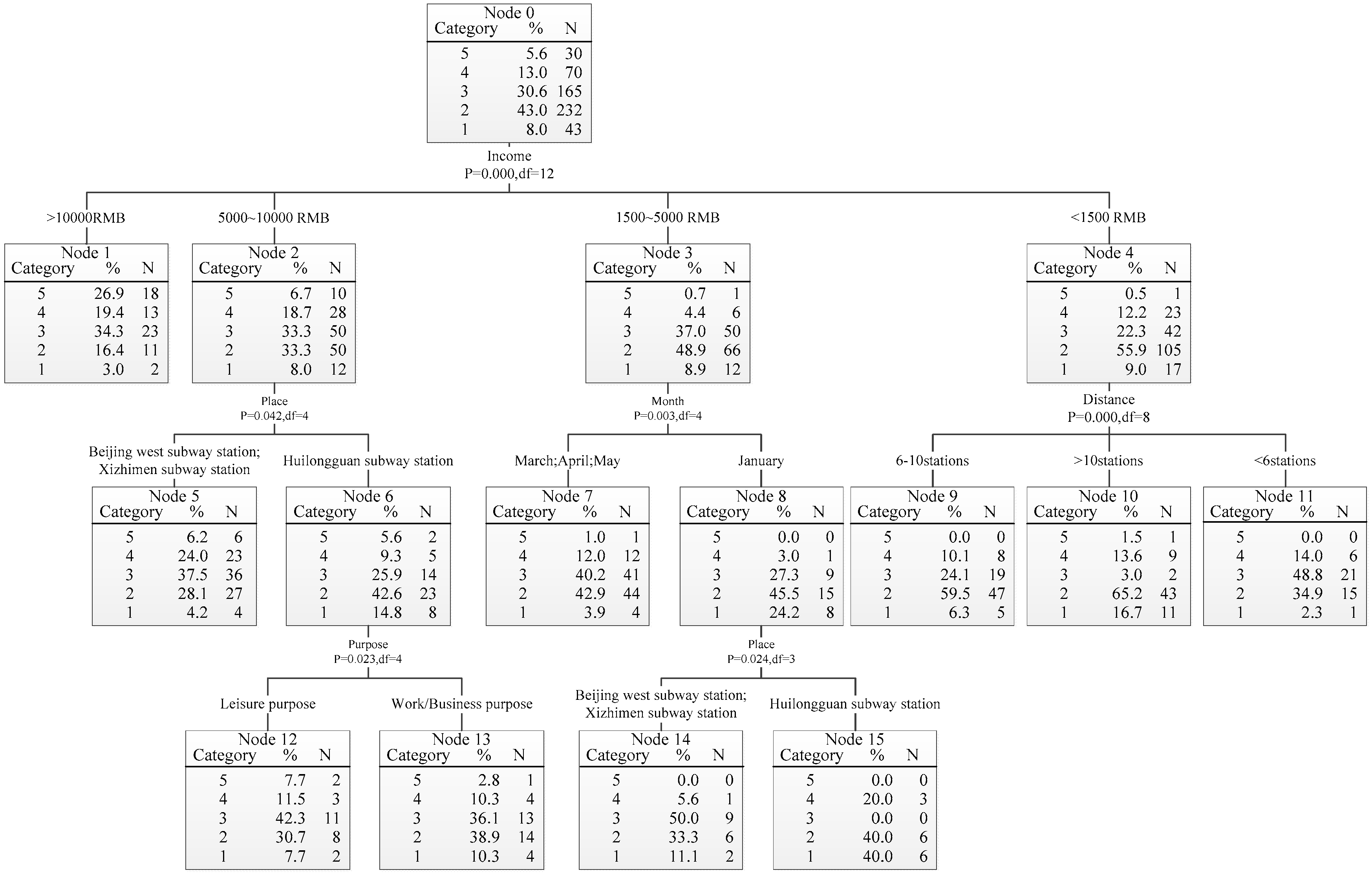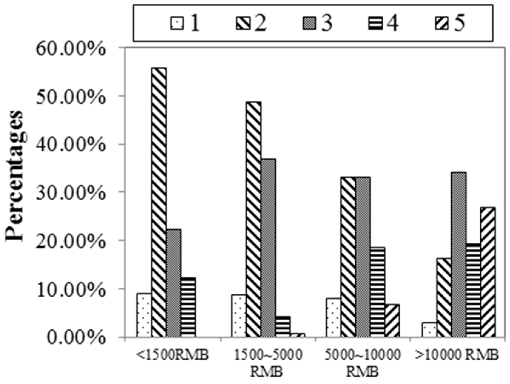Understanding passengers’ degree of satisfaction to a public transportation policy is particularly helpful for improving the mass transit service quality corresponding to specific public response [51]. In this paper, based on a survey analysis, it was found that most of the passengers are not pleased with the new Beijing subway fare policy and 42.96% of the respondents were dissatisfied with the policy. However, the degree of satisfaction became higher and higher over time after the policy implementation. Although the trend of the degree of satisfaction is obvious, the magnitude of the increment is low, indicating that it would take a long time for public to completely accept the new fare policy. From HTBR#1, it reveals that five factors, including income, place, month, distance and trip purpose have significant effects on the degree of satisfaction. It was found that low income riders were more inclined to be dissatisfied with the new policy and the difference in stations and trip purposes reflected that commuters were more dissatisfied with the policy than non-commuting passengers. The findings imply that the subway agency should take corresponding strategies, such as subsidizing low income people, commuters, or long distance travelers, to adapt to the new fare policy.

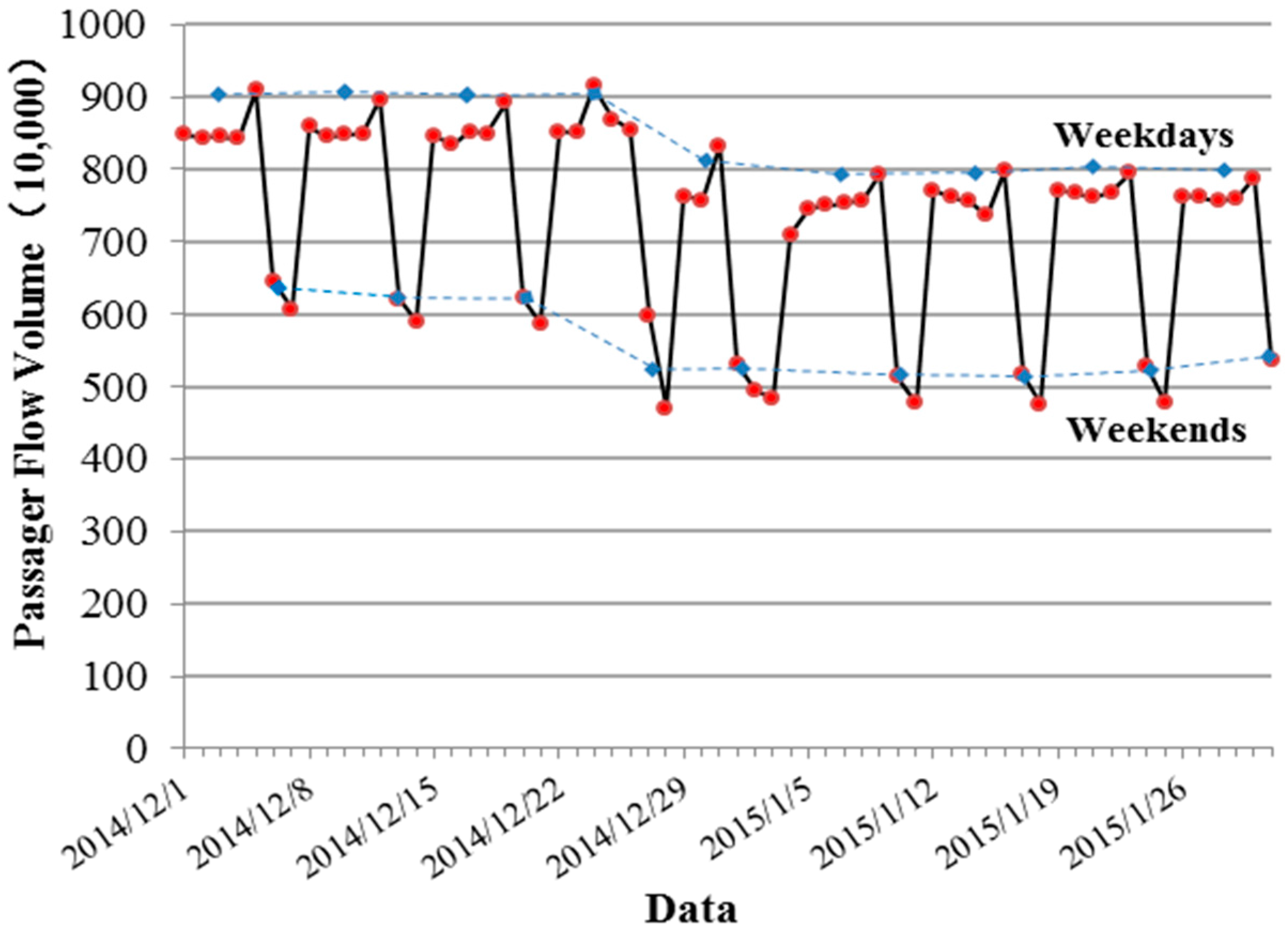
Although the degree of satisfaction could not be effectively recovered within five months after the new fare policy, the negative public attitude did not depress the subway demand continuously. Based on the time sequence analyses, the new policy made the ridership decrease sharply in the first month but gradually came back to the previous level four months later, and then the passenger flow volume kept steady again. To examine the impact of the new fare policy on the transit demand, Wang et al. predicted the demand and revenue associated with the new fare policy. They estimated that the fare policy would lead to losing almost half of its ridership but a revenue increase by 37.2% [28]. In fact, the results in this study indicate that there was only a short period effect rather than a significant impact on its ridership. One reason is that the previous “Two Yuan” fare per trip in Beijing subway was much lower than other countries’ prices and the new fare policy could not create an economic burden to the passengers based on their income levels in Beijing.

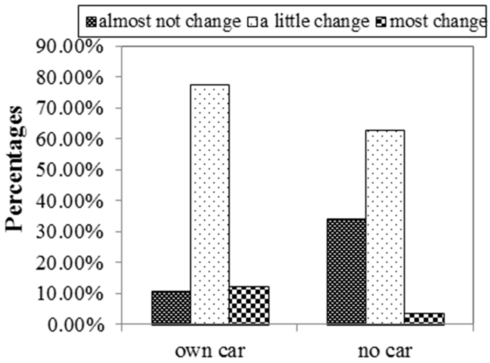
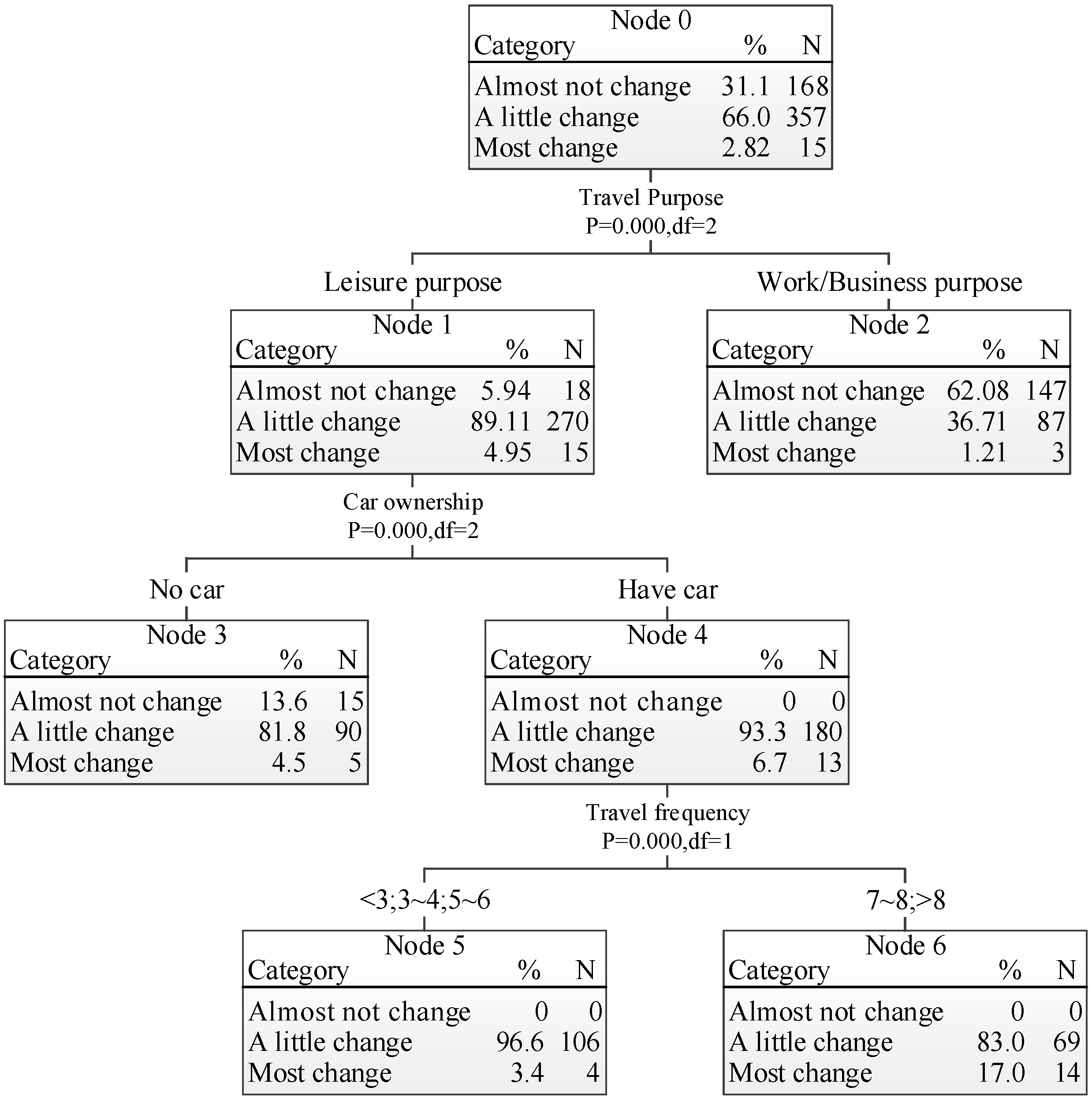
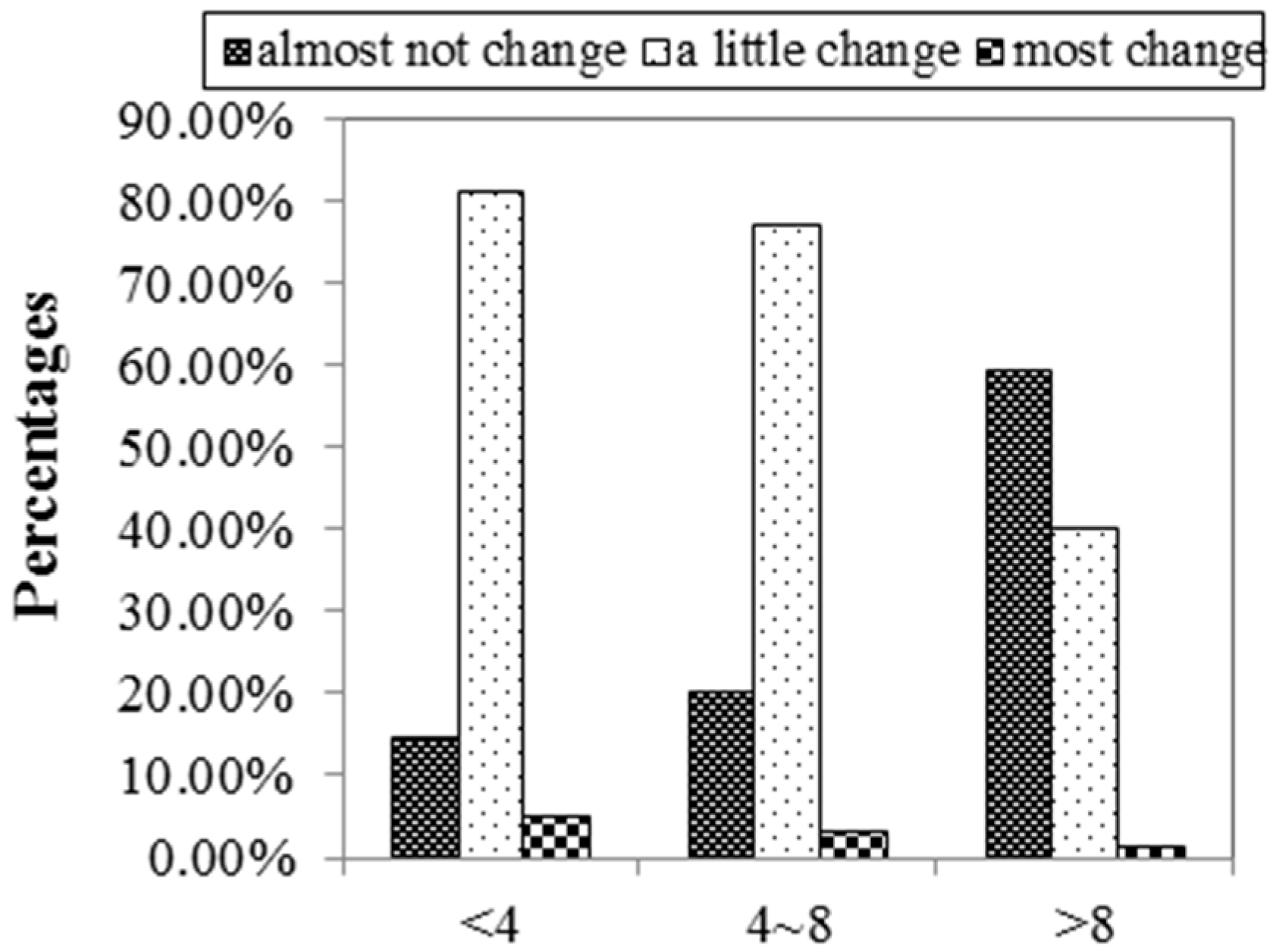
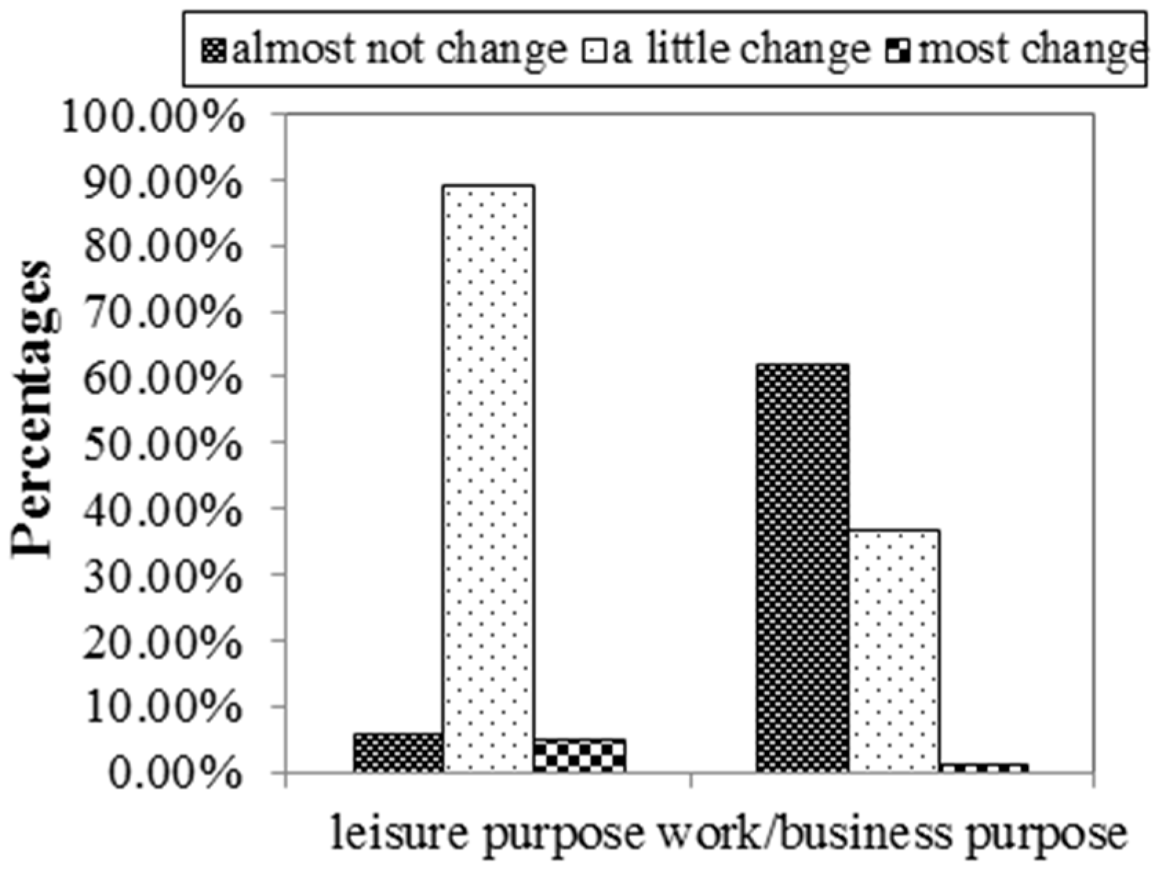
Prior empirical research showed that transit riders were sensitive to subway’s service quality as twice as fare change [52,53,54,55]. The survey results in this study indicated that most of the respondents chose “a little change” and only 2.78% of the respondents stated “major change” due to the new policy. HTBR#2 shows that travel frequency, travel purpose and car ownership have significant effects on the travel pattern change. The passengers who had cars were more likely to shift the public travel mode back to private vehicle usage. However, the captive riders who mainly rely on public transportation are less sensitive to fare changes than choice riders. For example, commuting trips during peak hours are less sensitive to fare change than discretionary ones [45].

The combination of the results of HTBR#1 and HTBR#2 provides a profound enlightenment on vertical equity. HTBR#1 shows that income, place, month, distance and trip purpose have significant impacts on the degree of satisfaction, while HTBR#2 displays that travel frequency, travel purpose and car ownership play a crucial role in the travel pattern change. It means that, although the passengers who are low-income travelers, commuters or long-distance traveler showed the most dissatisfied attitude on the new fare policy, they did not change their travel patterns mostly, indicating that they substantially relied on the public transport service and should be considered as the subsidized users.

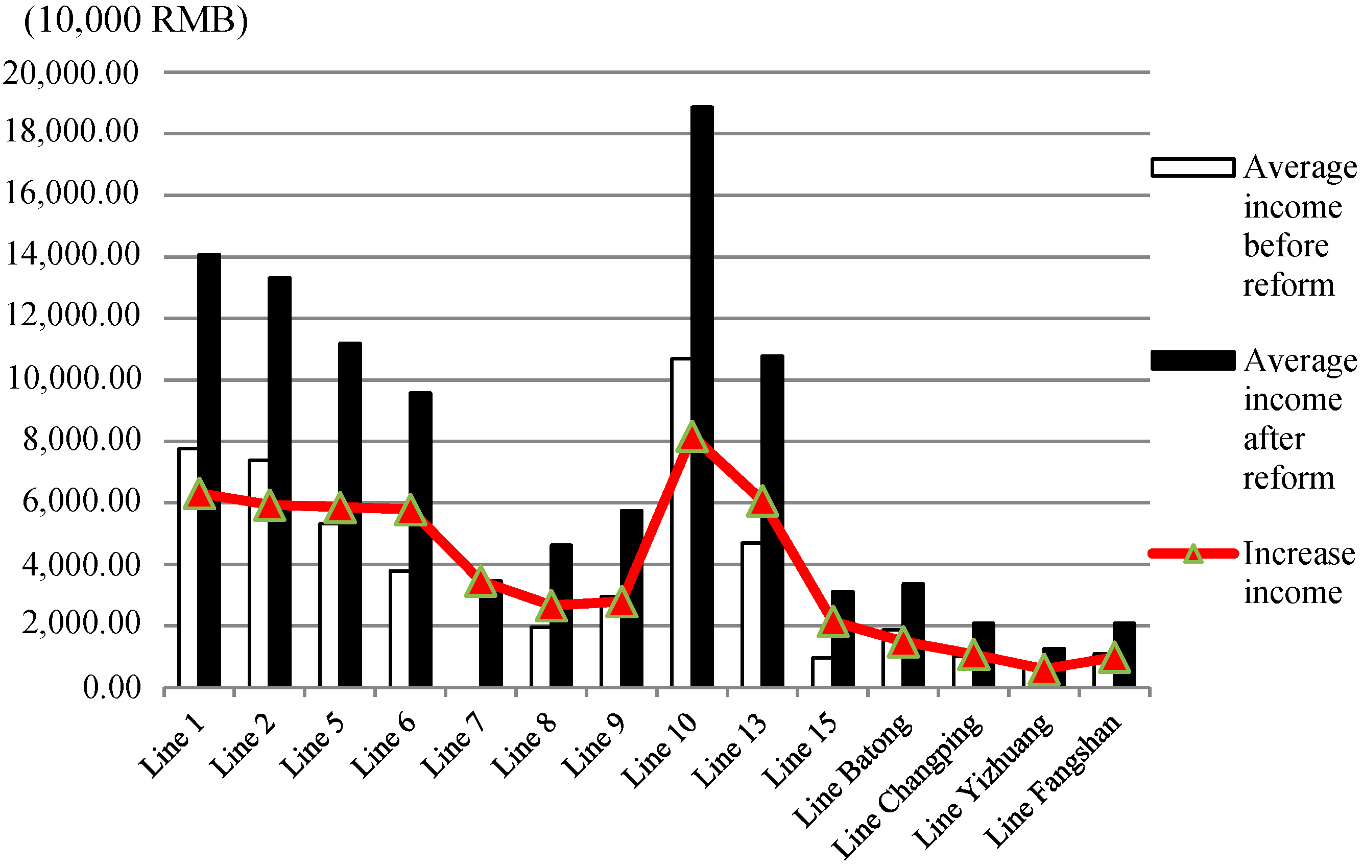
According to the Beijing Development and Reform Commission, after the Beijing subway fare policy reform, the average subway fare increased from 2 RMB to 4.3 RMB per trip [56]. According to the passenger flow volume in the Beijing subway system, the fare revenues for different subway lines can be estimated. Choosing half year from April to September as a comparison period between 2014 and 2015, Figure 12 shows that the average monthly fare income significantly increased after the new policy, especially on the high-volume lines, such as Line 10 whose revenue increased by about 80,000,000 RMB per month. In total, the increase of average monthly fare income could reach 533,796,800 RMB, which substantially reduced the government economy burden. Overall, the findings in this study indicate that the new fare policy realized the purpose of lowering the government’s financial pressure but could not reduce the subway ridership for long. After the new fare policy, the subway operation’s load factors in morning and evening rush hours are still high (even higher than 140%). Therefore, further improvements are needed to mitigate the safety concern caused by the overcrowded passenger flow. It was found that offering incentives to commuters such as reduced ticket fare during off peak hours have a positive influence on shifting rush-hour riders to off-peak period and a flexible work schedule has an impact on balancing the ridership demand and capacity of the subway system [57]. Additionally, this increased revenue could be used to improve the subway’s service quality, such as installing platform screen doors to enhance station safety level or increasing the trains’ capacity by adding compartments.

6. Conclusions

In this study, a survey analysis was conducted to identify the effects of the new fare policy for Beijing subway on riders’ satisfaction degree and travel pattern associated with the potential influencing factors using HTBR models. Further, the time series of the passenger flow volume were analyzed based on the ADF tests. The results show that income, distance and month have significant effects on the riders’ satisfaction degree to the fare policy; trip purpose, car ownership and travel frequency have a major influence on the travel pattern of the passengers. The ridership after the policy implementation decreased first, and then rebounded back within five months, indicating that the policy did not essentially influence the travel demand for Beijing subway but substantially mitigated the government’s financial pressure for maintaining the largest subway system in the world.

Limited by the data collection span, a five-month time series analysis of travelers satisfaction degree on the new fare policy might be not sufficient to reflect the whole process of their adaptability to a public transportation fee’s increasing. However, based on this study, it is suggested to more precisely formulate appropriate subsidized policies for the low-income travelers and commuters. The study results also indicate that the current subway facilities’ transportation capacity cannot sufficiently meet the rigid travel demand in Beijing. In the short term, how to effectively integrate bus and subway systems for coping with the public transportation issue should be an emerging research direction for urban transportation sectors.

References

1. Gkritza, K.; Karlaftis, M.G.; Mannering, F.L. Estimating multimodal transit ridership with a varying fare structure. Transp. Res. Part A 2011, 45, 148–160. [Google Scholar] [CrossRef]
2. Shen, W.; Xiao, W.; Wang, X. Passenger satisfaction evaluation model for Urban rail transit: A structural equation modeling based on partial least squares. Transp. Policy 2016, 46, 20–31. [Google Scholar] [CrossRef]
3. Paulley, N.; Balcombe, R.; Mackett, R.; Titheridge, H.; Preston, J.; Wardman, M.; Shires, J.; White, P. The demand for public transport: The effects of fares, quality of service, income and car ownership. Transp. Policy 2006, 13, 295–306. [Google Scholar] [CrossRef]
4. Webster, F.V.; Bly, P.H. The Demand for Public Transport; Report of an International Collaborative Study; Transport and Road Research Laboratory: Crow Thorne, UK, 1980. [Google Scholar]
5. Nuworsoo, C.; Golub, A.; Deakin, E. Analyzing equity impacts of transit fare changes: Case study of Alameda—Contra Costa Transit, California. Eval. Program Plan. 2009, 32, 360–368. [Google Scholar] [CrossRef] [PubMed]
6. Sharaby, N.; Shiftan, Y. The impact of fare integration on travel behavior and transit ridership. Trans. Policy 2012, 21, 63–70. [Google Scholar] [CrossRef]
7. Evans, J.E. IV. Transit Pricing and Fares: Traveler Response to Transportation System Changes; Publication TCRP Rep. 95, Chapter 12; Transportation Research Board: Washington, DC, USA, 2004. [Google Scholar]
8. Zureiqat, H.M. Fare Policy Analysis for Public Transport: A Discrete–Continuous Modeling Approach using Panel Data. Master’s Thesis, Massachusetts Institute of Technology, Cambridge, MA, USA, 2008. [Google Scholar]
9. Olsen, S.O. Repurchase loyalty: The role of involvement and satisfaction. Psychol. Mark. 2007, 24, 315–341. [Google Scholar] [CrossRef]
10. Lam, S.Y.; Shankar, V.; Erramilli, M.K.; Murthy, B. Customer value, satisfaction, loyalty, and switching costs: An illustration from a business-to-business service context. J. Acad. Mark. Sci. 2004, 32, 293–311. [Google Scholar] [CrossRef]
11. Chen, C.F. Investigating structural relationships between service quality, perceived value, satisfaction, and behavioral intentions for air passengers: Evidence from Taiwan. Transp. Res. Part A 2008, 42, 709–717. [Google Scholar] [CrossRef]
12. Jen, W.; Hu, K.C. Application of perceived value model to identify factors affecting passengers’ repurchase intentions on city bus: A case of the Taipei metropolitan area. Transportation 2003, 30, 307–327. [Google Scholar] [CrossRef]
13. Petrick, J.F. The roles of quality, value, and satisfaction in predicting cruise passengers’ behavioral intentions. J. Travel Res. 2004, 42, 397–407. [Google Scholar] [CrossRef]
14. Tyrinopoulos, Y.; Antoniou, C. Public transit user satisfaction: Variability and policy implications. Transp. Policy 2008, 15, 260–272. [Google Scholar] [CrossRef]
15. Eboli, L.; Mazzulla, G. Service quality attributes affecting customer satisfaction for bus transit. J. Public Transp. 2007, 10, 3. [Google Scholar] [CrossRef]
16. Eboli, L.; Mazzulla, G. A new customer satisfaction index for evaluating transit service quality. J. Public Transp. 2009, 12, 2. [Google Scholar] [CrossRef]
17. Friman, M.; Edvardsson, B.; Gärling, T. Frequency of negative critical incidents and satisfaction with public transport services. I. J. Retail. Consum. Serv. 2001, 8, 95–104. [Google Scholar] [CrossRef]
18. Hickey, R. Impact of transit fare increase on ridership and revenue: Metropolitan transportation authority, New York City. Transp. Res. Rec. 2005, 1927, 239–248. [Google Scholar] [CrossRef]
19. Cervero, R. Transit pricing research: A review and synthesis. Transportation 1990, 17, 117–139. [Google Scholar] [CrossRef]
20. Goodwin, P.B. A review of new demand elasticities with special references to short and long run effects of price charges. J. Transp. Econ. Policy 1992, 26, 155–170. [Google Scholar]
21. Hensher, D.A. Establishing a fare elasticity regime for urban passenger transport. J. Transp. Econ. Policy 1998, 32, 221–246. [Google Scholar]
22. Hensher, D.A. Assessing systematic sources of variation in public transport elasticities: some comparative warnings. Transp. Res. Part A 2008, 42, 1031–1042. [Google Scholar] [CrossRef]
23. Beijing Statistical Information Net. Available online: http://www.bjstats.gov.cn/ (accessed on 19 December 2016).
24. Chang, Z. Financing new metro—The Beijing metro financing sustainability study. Transp. Policy 2014, 32, 148–155. [Google Scholar] [CrossRef]
25. Beijing Subway Official Website. Available online: http://www.bjsubway.com/station/zjgls/ (accessed on 28 December 2014).
26. Zhang, G.; Liu, Y.; Xu, X.; Chen, F. Innovation of Investment and Financing Theory and Practice of Beijing’s Urban Rail Transit; Tsinghua University Press: Beijing, China, 2012. [Google Scholar]
27. Finance Bureau of Beijing (FBB). Report on Budget Execution of 2013 and Budget Draft of 2014 of Beijing. 2012. Available online: http://www.mof.gov.cn/zhuantihuigu/2014yshb/201402/t20140219_1044590.html (accessed on 19 February 2014).
28. Wang, Z.; Li, X.H.; Chen, F. Impact evaluation of a mass transit fare change on demand and revenue utilizing smart card data. Transp. Res. Part A 2015, 77, 213–224. [Google Scholar] [CrossRef]
29. Jiang, C.S.; Deng, Y.F.; Hu, C.; Ding, H.; Chow, W.K. Crowding in platform staircases of a subway station in China during rush hours. Saf. Sci. 2009, 47, 931–938. [Google Scholar] [CrossRef]
30. Mahudin, N.D.M.; Cox, T.; Griffiths, A. Measuring rail passenger crowding: Scale development and psychometric properties. Transp. Res. Part F 2012, 15, 38–51. [Google Scholar] [CrossRef]
31. Mayeres, I.; Ochelen, S.; Proost, S. The marginal external costs of urban transport. Transp. Res. Part D 1996, 1, 111–130. [Google Scholar] [CrossRef]
32. Sposato, R.G.; Röderer, K.; Cervinka, R. The influence of control and related variables on commuting stress. Transp. Res. Part F 2012, 15, 581–587. [Google Scholar] [CrossRef]
33. Xinhua Net1. Available online: http://news.xinhuanet.com/local/2014-12/28/c_1113799711.htm (accessed on 28 December 2014).
34. Tao, H. Metro should Increase Fare as Well as Other Measures; International Monetary Institute of Renmin University of China: Beijing, China, 2014. [Google Scholar]
35. Cai, S.; Jiang, Y. Inquiring into a ticketing price scheme of Beijing Metro. J. Transp. Syst. Eng. Inf. Technol. 2002, 3, 44–47. [Google Scholar]
36. Gao, M. Discussion on metro ticket pricing and reform strategy—Take Beijing Subway for an example. Price Mon. 2014. [Google Scholar] [CrossRef]
37. Delbosc, A.; Currie, G. Using Lorenz curves to assess public transport equity. J. Transp. Geogr. 2011, 19, 1252–1259. [Google Scholar] [CrossRef]
38. Litman, T. Evaluating transportation equity. World Transp. Policy Pract. 2002, 8, 50–65. [Google Scholar]
39. Lowe, J.C.; Altshuler, A.; Womaek, J.P.; Pucher, J.R. The urban transportation system: Politics and policy innovation. Econ. Geogr. 1980, 56, 81–82. [Google Scholar] [CrossRef]
40. Rock, S.M. Redistributive Effects of Public Transit: Framework and Case Study. 1976. Available online: https://trid.trb.org/view.aspx?id=65687 (accessed on 26 April 2017).
41. Cervero, R. Flat versus differentiated transit pricing: What’s a fair fare? Transportation 1981, 10, 211–232. [Google Scholar] [CrossRef]
42. Farber, S.; Bartholomew, K.; Li, X.; Páez, A.; Nurul Habib, K.M. Assessing social equity in distance based transit fares using a model of travel behavior. Transp. Res. Part A 2014, 67, 291–303. [Google Scholar] [CrossRef]
43. Karlaftis, M.G.; Golias, I. Effects of road geometry and traffic volumes on rural roadway accident rates. Accid. Anal. Prev. 2002, 34, 357–365. [Google Scholar] [CrossRef]
44. Chang, L.Y.; Chen, W.C. Data mining of tree-based models to analyze freeway accident frequency. J. Saf. Res. 2005, 36, 365–375. [Google Scholar] [CrossRef] [PubMed]
45. Stewart, J. Applications of classification and regression tree methods in roadway safety studies. Transp. Res. Rec. 1996, 1542, 1–5. [Google Scholar] [CrossRef]
46. Wets, G.; Vanhoof, K.; Arentze, T.; Timmermans, H. Identifying decision structures underlying activity patterns: An exploration of data mining algorithms. Transp. Res. Rec. 2000, 1718, 1–9. [Google Scholar] [CrossRef]
47. Yamamoto, T.; Kitamura, R.; Fujii, J. Drivers’ route choice behavior: Analysis by Data mining algorithms. Transp. Res. Rec. 2002, 1807, 59–66. [Google Scholar] [CrossRef]
48. Hallmark, S.L.; Guensler, R.; Fomunung, I. Characterizing on-road variables that affect passenger vehicle modal operation. Transp. Res. Part D 2002, 7, 81–98. [Google Scholar] [CrossRef]
49. Friedman, J.; Hastie, T.; Tibshirani, R. The elements of statistical learning. In Springer Series in Statistics; Springer: Berlin, Germany, 2001. [Google Scholar]
50. Kremers, H.; Nijkamp, P.; Rietveld, P. A meta-analysis of price elasticity of transport demand in a general equilibrium framework. Econ. Model. 2002, 19, 463–485. [Google Scholar] [CrossRef]
51. Ji, J.; Gao, X. Analysis of people’s satisfaction with public transportation in Beijing. Habitat Int. 2010, 34, 464–470. [Google Scholar] [CrossRef]
52. Morgan, J.N.; Sonquist, J.A. Problems in the analysis of survey data, and a proposal. J. Am. Statist. Assoc. 1963, 58, 415–434. [Google Scholar] [CrossRef]
53. Kemp, M.A. Some evidence of transit demand elasticities. Transportation 1973, 2, 25–52. [Google Scholar] [CrossRef]
54. Dygert, P.; Holec, J.; Hill, D. Public Transportation Fare Policy; U.S. Department of Transportation: Washington, DC, USA, 1977.
55. Mayworm, P.D.; Lago, A.M.; McEnroe, J.M. Patronage Impacts of Changes in Transit Fares and Services; Urban Mass Transportation Administration: Washington, DC, USA, 1980.
56. Xinhua Net2. Available online: http://news.xinhuanet.com/politics/2014-10/28/c_127147473.htm (accessed on 28 October 2014).
57. Zhang, Z.; Fujii, H.; Managi, S. How does commuting behavior change due to incentives? An empirical study of the Beijing Subway System. Transp. Res. Part F 2014, 24, 17–26. [Google Scholar] [CrossRef]
Figure 1. Beijing Subway Map.
Sustainability 09 00689 g001
Figure 2. Relationship between Month and Degree of Satisfaction.
Sustainability 09 00689 g002
Figure 3. Relationship between Distance and Degree of Satisfaction.
Sustainability 09 00689 g003
Figure 4. Relationship between Income and Degree of Satisfaction.
Sustainability 09 00689 g004
Figure 5. Relationship between Travel Frequency and Travel pattern change.
Sustainability 09 00689 g005
Figure 6. Relationship between Travel Purpose and Travel pattern change.
Sustainability 09 00689 g006
Figure 7. Relationship between Car Ownership and Travel pattern change.
Sustainability 09 00689 g007
Figure 8. Hierarchical Tree-Based Regression (HTBR) Model #1—classifying the degree of satisfaction.
Sustainability 09 00689 g008
Figure 9. HTBR Model #2—classifying the travel pattern change.
Sustainability 09 00689 g009
Figure 10. Beijing subway total passenger flow volume series.
Sustainability 09 00689 g010
Figure 11. Beijing subway passenger flow volume series frame.
Sustainability 09 00689 g011
Figure 12. Fare income of different subway line.
Sustainability 09 00689 g012