Spatial Prediction of Soil Organic Matter Using a Hybrid Geostatistical Model of an Extreme Learning Machine and Ordinary Kriging

Abstract

An accurate estimation of soil organic matter (SOM) content for spatial non-point prediction is an important driving force for the agricultural carbon cycle and sustainable productivity. This study proposed a hybrid geostatistical method of extreme learning machine-ordinary kriging (ELMOK), to predict the spatial variability of the SOM content. To assess the feasibility of ELMOK, a case study was conducted in a regional scale study area in Shaanxi Province, China. A total of 472 topsoil (0–20 cm) samples were collected. A total of 14 auxiliary variables (predictors) were obtained from remote sensing data and environmental factors. The proposed method was compared with the ability of traditional geostatistical methods such as simple kriging (SK) and ordinary kriging (OK), in addition to hybrid geostatistical methods such as regression-ordinary kriging (ROK) and artificial neural network-ordinary kriging (ANNOK). The results showed that the extreme learning machines (ELM) model used principal components (PCs) as input variables, and performed better than both multiple linear regression (MLR) and artificial neural network (ANN) models. Compared with geostatistical and hybrid geostatistical prediction methods of SOM spatial distribution, the ELMOK model had the highest coefficient of determination (R² = 0.671) and ratio of performance to deviation (RPD = 2.05), as well as the lowest root mean square error (RMSE = 1.402 g kg⁻¹). In conclusion, the application of remote sensing imagery and environmental factors has a deeper driven significance of a non-linear and multi-dimensional hierarchy relationship for explaining the spatial variability of SOM, tracing local carbon sink and high quality SOM maps. More importantly, it is possibly concluded that the sustainable monitoring of SOM is a significant process through the pixel-based revisit sampling, an analysis of the mapping results of SOM, and methodological integration, which is the primary step in spatial variations and time series. The proposed ELMOK methodology is a promising and effective approach which can play a vital role in predicting the spatial variability of SOM at a regional scale.

1. Introduction

With rising concern regarding soil organic matter (SOM), it has generally been considered as a critical indicator of agricultural sustainability [1]. SOM directly affects the sustainability of soil quality such as soil nutrients and soil texture. It also indirectly impacts carbon emissions and, in turn, climate change, which limits the productive forces of food and the carrying capacity of the ecological environment [2,3,4]. That is, the sustainable connotation of SOM can be defined as: the SOM in the land unit meets the needs and aspirations of the food productivity of the present, which coordinates with the development of population growth and resource utilization without compromising the ability of future generations to meet their own food needs [5,6]. With respect to the spatial variability of SOM and associated disturbances (such as warming or land use change) for soil quality, digital soil mapping is an effective way to estimate the value of a non-sampled area and to acquire the spatial variation of SOM [7]. Furthermore, the soil mapping of SOM can improve the response time of disturbances and the efficiency of the analysis of sustainable monitoring. Simultaneously, pixel-based mapping of SOM can be more easily displayed at higher resolutions, and reduces the cost and time required for field sampling by reducing the amount of sampling.

Selecting appropriate auxiliary variables is crucial for gaining a better understanding of soil properties, which are closely related to the predicted precision and sustainable space-time fitting for SOM. The most common of such auxiliary variables are environmental factors that are easy to obtain such as climate, vegetation, topography, and soil type [8,9,10,11]. However, it is hard to obtain a high prediction accuracy of SOM content when only considering environmental variables at the local scale, because there is less spatial variation and a weak nonlinear relationship. In recent years, remote sensing (RS) data has also been used to estimate the spatial variability of SOM because of the advantage of its multi-spectrum feature, which has a satisfactory forecast effect [12,13]. Remote sensing variables have a better spatial transitivity, but do not easily explain the driving mechanism behind global change and the carbon sink of SOM in comparison with environmental variables. Furthermore, few researchers simultaneously consider the RS data and the environmental variables, especially the potential driving force among various factors and the expression of geographical connotations that are applied to establish the prediction models, and the target data has a limited number of laboratory observations of SOM. Therefore, it is of great importance to adequately develop theoretical approaches for predicting the spatial variability of SOM from multi-source auxiliary variables (multi-spectral data and other environmental factors) that are thoroughly taken into account in the modeling process.

The high-efficiency quantitative model is an indispensable technique for predicting the spatial variability of soil properties, which is based on the application of multi-source auxiliary variables [14]. The explanatory ability of spatial variability between soil properties and auxiliary variables can be efficiently described using traditional geostatistical methods such as simple kriging (SK), ordinary kriging (OK), universal kriging (UK), and cokriging (CK) [15,16,17]. As a widely applicable method, kriging interpolation has achieved a certain effect between observations and auxiliary variables using spatial correlation and variation functions [18,19,20]. However, it is difficult to determine the low degree of non-linear fitting between SOM and assistant variables because of the interference of sampling density and the spatial autocorrelation of the multi-dimensional data. In recent years, hybrid geostatistical methods that integrate a linear or non-linear algorithm and geostatistics methodology have been broadly employed in different spatial productions of soil properties. Regression kriging (RK) and neural network kriging (NNK) are typical modeling approaches of hybrid geostatistical methods [21,22,23]. RK uses the summation of both regression values, which represent the approximate ability between the soil dependent variable and auxiliary parameters, and kriging values of the regression residuals, which reflect the spatial autocorrelation of the soil properties [24,25,26]. Many RK applications have shown that RK has a better imitative effect than the single kriging methods due to its simplicity, computational efficiency, and linear analysis ability [27,28]. In fact, RK still displays a low prediction accuracy because of its weak analytical ability in non-linear relationships and layer structures between target data and multi-source auxiliary variables. Since the development of artificial intelligence and machine learning, neural networks (NN) have been used to solve the complex non-linear problems between soil properties and auxiliary variables, which results in a higher precision than when using classic linear methods [29,30,31]. However, traditional artificial neural networks (ANN) have a low implementation efficiency, which is needed to adjust the complex parameters from the algorithm structure and to avoid the influence of a locally optimal solution; in particular, they require a longer running time when the mapping resolution is increased. Furthermore, a more efficient method is required to produce a significant advantage in terms of the operation time, generalization quality, and layer-interrelating analysis between SOM and multi-source auxiliary variables.

An extreme learning machine (ELM) is a single layer feed forward neural network (SLFN) which was proposed by Huang (2004), and has the same single hidden layer structure as traditional NN [32,33]. The ELM algorithm has gradually been employed to determine soil properties such as soil heavy metals, soil temperature, and soil moisture, due to its excellent generalization performance and global optimal property [34,35,36]. Most prominently, ELM has a faster learning speed than classical artificial neural networks (ANN) because it simplifies the training processes by randomly selecting the parameters. Extreme learning machine ordinary kriging (ELMOK) calculates both ELM values, which represent the approximate ability between the soil dependent variables and auxiliary parameters, and the ordinary kriging values of the ELM residuals, which reflect the spatial autocorrelation of the soil properties. However, little research has been conducted to explain the importance of auxiliary factors for the spatial variation of SOM and to infer the geographical significance of hybrid geostatistical methods from the aspect of their non-spatial algorithm essence. Therefore, the objective of this study was to adopt a new integrating model of ELMOK combined with principal component analysis, and to compare it with the performance of different geostatistical and hybrid geostatistical models for SOM content mapping, simultaneously using RS data and environmental variables.

2. Materials and Methods

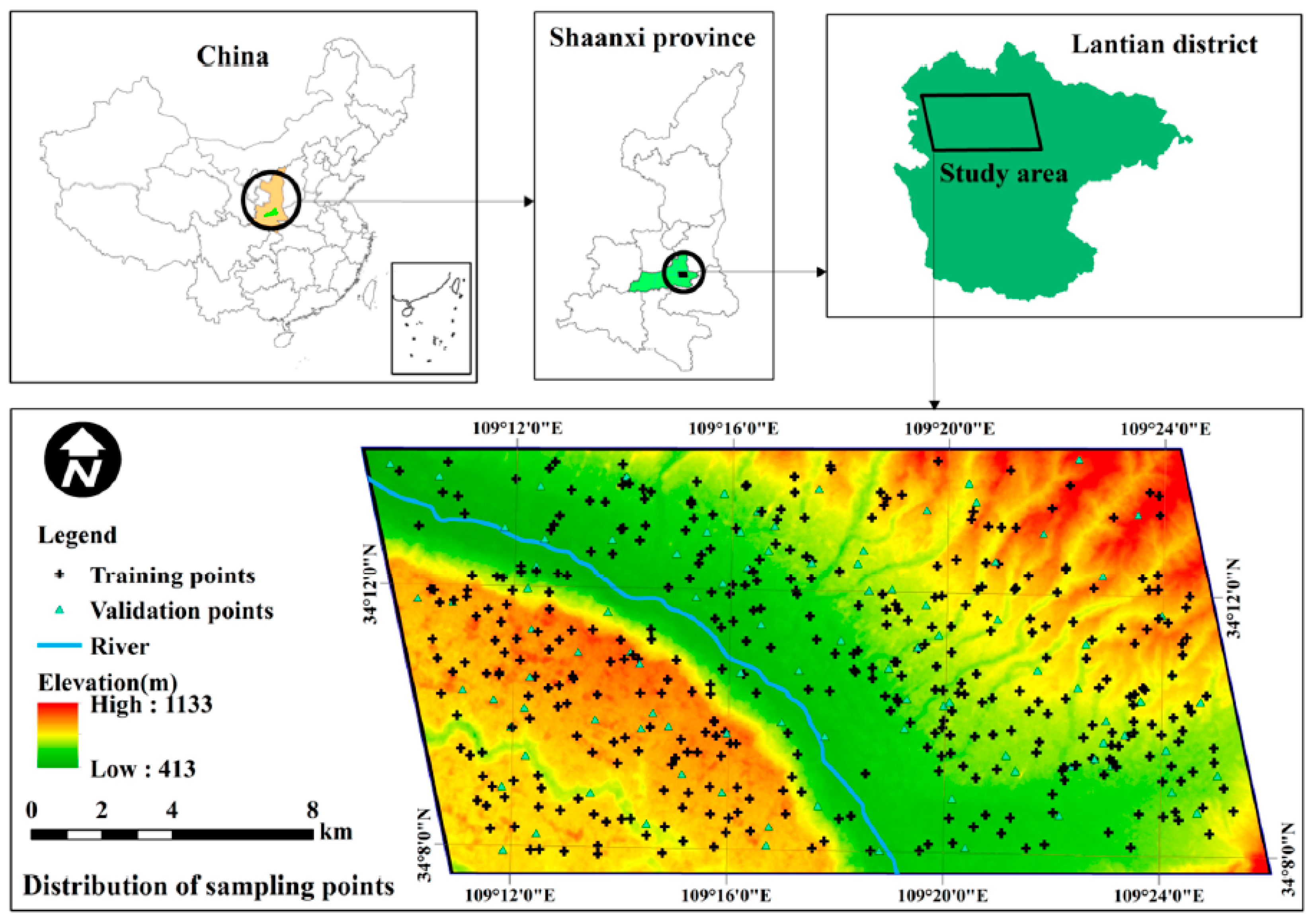
2.1. Study Area

The study area (33°50′ to 34°19′N and 109°07′ to 109°49′E) is located in the southeast of Xi’an, Shannxi, China (Figure 1). We chose an area of approximately 305 km², of which nearly 70% is earmarked for agricultural production. The climate of the study area is a continental monsoon with a mean annual temperature of 13.1 °C, a mean annual sunshine hours of 2148.8 h, and a mean annual precipitation of 720.4 mm, of which nearly 85% falls from July to September. The topography is plain and hilly, with an elevation ranging from 410 m to 2449 m. According to Chinese soil classification, the main soil types of vegetable fields are brown soils and cinnamon soils (Dystrochrept and half ustalf in the USDA Soil Taxonomy; Eutric luvisd and unsaturated cambisol in the FAO World Reference Base for Soil Resources). This area is a historic agricultural zone in the central Shaanxi plain, where the dominant planting structure is an irrigated farming system producing wheat, corn, and vegetables.

2.2. Soil Sampling and Analysis

It is essential that sampling occurs during the driest months, after crops have been harvested, to reduce the interference of soil moisture, soil texture, cloud cover, and vegetation for the multi-spectral information of the remote sensor. The base map of field sampling was overlaid pattern spots by the present land-use map and soil type map (from the Lantian County Agricultural Technology Popularization Center, China). Based on the sampling requirements of the “Rules for soil quality survey and assessment, NY/T 1634-2008” [37], which was released by the Ministry of Agriculture of the People’s Republic of China, they set one point per 66.66 ha and the topsoil depth is from 0 cm to 20 cm. We combined this with the actual situation of the study area, used a uniform random sampling technique, and set one point per 60 ha. However, the sampling points should avoid the interference of the land type such as buildings, ditches, scrap heaps, dunghills, cemeteries, and so on, whilst the distance from a railway or main street should exceed 350 m. A total of 472 topsoil (0–20 cm) samples (Figure 1) were collected over the study area in November 2012, taking the coordinates, soil type, and topography into consideration. All soil mixed samples included four corners of a square within a 10 m length, each of approximately 2 kg, and these were mixed thoroughly. This was developed in accordance with the technical requirements of the “Chinese agriculture Industry standard, NY/T 1211.1-2006” [38] for measured soil organic matter, which was released by the Ministry of Agriculture of the People’s Republic of China. All samples were naturally air dried at room temperature and passed through a 2-mm nylon sieve after removing plant residues and stones. In the analytic procedure, samples were oxidized by 0.4 mol L⁻¹ potassium dichromate-sulfuric acid, then heated to about 170–180 °C for 5 min ± 0.5 min, and any excess potassium dichromate was determined by titration with standard 0.1 mol L⁻¹ ferrous sulfate (FeSO₄). Meanwhile, two blank experiments were completed when analyzing each batch of samples. The SOM content was calculated by the conventional carbon factor (1.724), as follows [39,40]:

$$\mathrm{SOM}=\frac{c\times (V_0-V)\times 0.003\times 1.724\times 1.10}{m}\times 1000$$

(1)

where SOM is the soil organic matter content (g kg⁻¹), V₀ is the consumption volume of the ferrous sulfate standard solutions in the blank experiments (mL), V is the consumption volume of the ferrous sulfate standard solutions in the sample determination (mL), c is the concentration of ferrous sulfate standard solution (mol L), 0.003 is the millimole mass of a quarter of the carbon atoms (g), 1.724 is the conventional carbon factor, 1.10 is the oxidation adjusting coefficient, m is the mass of the dry samples (g), and 1000 is the content of per kilogram conversion.

2.3. Auxiliary Variables

A Landsat 8 OLI image with nine bands was freely obtained from the National Aeronautics and Space Agency (NASA) server at a spatial resolution of 30 m by 30 m (the eighth band is 15 m) [41]. We selected the OLI image of December 2014 from November 2012 to December 2015 as it had the least cloud cover and avoided the information interference from the black stripe of Landsat 7 ETM+. The OLI image was geo-referenced to the same coordinate system as the SOM data set and was processed through radiometric calibration and atmospheric correction in ESRI ENVI 5.2 (ESRI Inc., Redlands, CA, USA). The selected remote sensing auxiliary variables included a blue band (band 2), green band (band 3), red band (band 4), NIR (band 5), SWIR (bands 6 and 7), and the normalized difference vegetation index (NDVI) [42].

In this study, we used a digital elevation model (DEM) with a spatial resolution of 30 m, which was obtained from Advanced Spaceborne Thermal Emission and Reflection Radiometer Global Digital Elevation Model version 2 (ASTER GDEMV2). The dataset was provided by the International Scientific & Technical Data Mirror Site, Computer Network Information Center, Chinese Academy of Sciences [43]. Furthermore, four topographic variables were derived from the DEM: (1) elevation (ELE, m), (2) slope (SLO, °), (3) aspect (ASP), and (4) relief (REL, m). All of these terrain variables were calculated using 3D analysis tools in ArcGIS 10.3 (ESRI Inc., Redlands, CA, USA).

Climate variables with a 1 km spatial resolution were derived from the Geospatial Data Cloud of China, which included the monthly total precipitation and monthly mean temperature. These data were further applied to calculate the average monthly precipitation (PREC, mm) and average monthly temperature (TMEAN, °C). In order to use the same spatial resolution for the DEM and that used in the subsequent analysis, the PREC and TMEAN were resampled to a 30 m spatial resolution, according to the nearest neighbor assignment method in ArcGIS 10.3. The soil potential of hydrogen (pH) was obtained from the mixed soil samples. The determination of the soil pH was achieved through a calomel electrode with a sleeve type connection, which was interpolated into raster maps at a 30 m resolution by the inverse distance weighted (IDW) method as soil property data [44].

2.4. Dimension-Reduced Processing

Since a reasonable amount and type of auxiliary variables not only simplifies the model structure, but also analyzes the driving force of different variables, environmental variables and remote sensing data were simultaneously considered to predict the spatial variability of soil organic matter (SOM). In this study, the combined method of stepwise linear regression and principal component analysis (SLR-PCA) was used for the dimension reduction processing of the auxiliary variables. The stepwise linear regression (SLR) method is usually used to solve the linear relationship between multiple independent variables, which can be applied as a type of variable screening to build subsequent prediction models by removing weak significant variables and retaining high contribute rate variables. Stepwise regression is adopted to eliminate variables step by step, and to find the optimal combination of variables in a multi-variable regression relationship. Furthermore, principal component analysis (PCA) was applied to reduce the dimensions of the quantitative auxiliary variables after SLR analysis, in order to remove their multi-collinearity and normalized initial number within the range of 0.1–0.9 using Equation (2). The selected principal components (PCs) were constructed from linear combinations of independent variables, which explained at least 80% of the total variance among the original data sets. Afterwards, these PCs were used as input variables in the subsequent modeling prediction of SOM. The SLR-PCA were performed with SPSS, version 22.0, 2013.

$$x_i=0.8\times \left[\frac{(x-x_{\min })}{x_{\max }-x_{\min }}\right]+0.1,$$

(2)

where x_i is the rescaled data, and x_min and x_max are the minimum and maximum observed data, respectively.

2.5. Modeling MLR, ANN and ELM

In regression analysis, a multiple linear regression approach (MLR) was introduced to explore the spatial variability of the soil organic matter (SOM) content with auxiliary variables by a least square algorithm. As a linear equations fitting method, MLR generally found the appropriate equation for the relationship between the input PCs and target data, and then resolved the coefficients of the fitting polynomial [19]. The artificial neural network (ANN) is a feed-forward multi-layer perceptron which originated from the abstract neuron structure in the biological brain. Generally, the ANN model has three layers (input layer, hidden layer, and output layer), which were used to estimate the non-linear fitting relationship between SOM and multi-source auxiliary variables. The multiple linear regression and ANN processes were performed using the MATLAB 2013b software (MathWorks, Natick, MA, USA). Compared to the traditional function structure of ANN, the extreme learning machine (ELM) does not require bias parameters in the output layer or the training of a multi-layer perceptron with one hidden layer, which is equivalent to simply finding the least-squares solution of the linear system. The output function of the SLFN of ELM can be defined as follows:

$$f_L(x)={\displaystyle \sum _{i=1}^L{\beta }_{i}h(w_i\cdot x_j+b_i)=h(x)\beta },$$

(3)

where $x\in R^d$ and $f_L(x)\in R^m$ are the model input and output, respectively; N is the number of input vectors; $w_i$ is the weight in the hidden layer; and $b_i$ represents the bias parameters in the hidden layer. β = [β₁, …, β_L]^T is the output weight vector between the hidden layer of L nodes to the output nodes of m; $h(x)=\left[h_1(x),\hspace{0.17em}\hspace{0.17em}\cdots \hspace{0.17em}\hspace{0.17em},h_L(x)\right]$ is the nonlinear feature mapping relation of ELM, with respect to the input data from the row output vector of the hidden layer; and $h(w_i\cdot x_j+b_i)$ is the output function of the ith hidden node, which can be written as follows:

$$h(w_i\cdot x_j+b_i)=G(w,b,x),$$

(4)

where $G(w,b,x)$ represents the nonlinear mapping of continuous functions, namely the activation function.

In the next stage of ELM learning, Equation (5) is used to minimize the approximation error in the squared error sense between the hidden layer and the output layer:

$$\underset{\beta \in R^{L\times m}}{\min }{||H\beta -T||}^2,$$

(5)

where $||\cdot ||$ denotes the Frobenius norm, H is the hidden layer output matrix (random matrix) of dimension N × L, T is the training data target matrix, and superscript T denotes the transpose.

The optimal least square solution can be calculated as follows:

$$\widehat{\beta }={\mathrm{H}}^{†}\mathrm{T},$$

(6)

where H^† is the Moore-Penrose generalized inverse of output matrix H.

The ELM algorithm has advantages in terms of the training time and accuracy via improving the training data by converting them into batches of a fixed or not fixed length, and only updating the weight without retraining the trained samples. The MATLAB 2013b software was used in ELM modeling analysis.

2.6. Hybrid Geostatistical Methods

The hybrid geostatistical methods including regression-ordinary kriging (ROK), artificial neural network-ordinary kriging (ANNOK), and extreme learning machine-ordinary kriging (ELMOK), integrate a non-spatial method (MLR, ANN, and ELM models) and a spatial interpolation approach of ordinary kriging. The implementation of these methods includes three steps: Firstly, the MLR, ANN, and ELM model between the target data and the PCs which is derived from the initial auxiliary variables is established; secondly, the residuals of MLR, ANN, and ELM are computed by a semivariogram and kriging, respectively; and finally, the prediction of each non-spatial method and the ordinary kriging prediction of the residual is calculated.

The implementation of residual kriging is achieved according to the MLR, ANN, and ELM prediction, and a residual error can be written as follows:

$$r(x_i)=Z(x_i)-\widehat{Z}(x_i),$$

(7)

where $r(x_i)$ is the residual error at the sampling site $x_i$; $Z(x_i)$ is the measured value; and $\widehat{Z}(x_i)$ represents the estimation data by the MLR, ANN, and ELM model, respectively. The OK method is given by:

$$\widehat{r}(x_i)={\displaystyle \sum _{i=1}^n{\lambda }_{i}r(x_i)},$$

(8)

where $\widehat{r}(x_i)$ is the estimated $r$ at a site $x_i$ with ordinary kriging. $r(x_i)$ and $n$ are the MLR or ELM residual values at site $x_i$ and the number of soil samples, respectively, and ${\lambda }_i$ is the optimal weight. In the spatial modeling of residual kriging, an experimental semivariogram is usually used to measure the average dissimilarity between the points separated through a lag distance, which is defined as follows:

$$\widehat{\gamma }(h)=\frac{1}{2N(h)}{\displaystyle \sum _{i=1}^{N(h)}{\left[r(x_i)-r(x_i+h)\right]}^2},$$

(9)

where $\widehat{\gamma }(h)$ is the experimental semivariogram, which is measured by the lag distance $h$ between $r(x_i)$ and $r(x_i+h)$, and $N(h)$ is the number of pairs of sampling sites separated by $h$. ArcGIS 10.3 was used to implement the spatial interpolation and geostatistical computations.

Finally, the hybrid geostatistical methods of ROK, ANNOK, and ELMOK were obtained as the respective sum of the $\widehat{Z}(x_i)$ (representing MLR estimates, ANN estimates, and ELM estimates, respectively) and ordinary kriging estimates of the residuals $\widehat{r}(x_i)$, as follows:

$${\widehat{Z}}_{sum}(x_i)=\widehat{Z}(x_i)+\widehat{r}(x_i),$$

(10)

where ${\widehat{Z}}_{sum}(x_i)$ (including ROK, ANNOK, and ELMOK models) is the final spatial optimum estimation of the SOM content.

2.7. Accuracy Evaluation of Prediction Performance

In order to evaluate the prediction results and the performance of different modeling methods, four quantitative measures of the mean error (ME), root mean square error (RMSE), coefficient of determination (R²), and ratio of performance to deviation (RPD) were computed in this study. The formulas of the RPD indexes were calculated as follows:

$$\mathrm{RPD}=\frac{\mathrm{STD}}{\mathrm{RMSE}},$$

(11)

where STD is the standard deviation of the SOM measurement (g kg⁻¹), the increasing RPD values mean that the quality of the prediction model can be interpreted more accurately according to three classes: the accurate prediction of the model (RPD ≥ 2), the fairly acceptable prediction (1.4 < RPD < 2), and the worst performance of the prediction model (RPD ≤ 1.4) [45,46].

An independent test data set (142 samples, 30% of the total) was randomly conducted by using the “create subset” function of Geostatistical Analyst in ArcGIS 10.3. The ELMOK is a pixel-based mapping method that needs a one-to-one correspondence between the pixel value of the auxiliary variables and the samples of SOM. Once the validation set was changed, the training set and the corresponding pixel value of the auxiliary variables were changed accordingly. Not only did it need to re-modeled and re-trained as the model lacked robustness and stability, but it also avoided over-fitting because the sample variations disrupted the one-to-one relationships between the pixel value of the auxiliary variables and the samples of SOM. In other words, the first subset produced was random, yet the validation set was independent in the subsequent process of modeling analysis [14,31].

3. Results

3.1. Descriptive Statistics

Table 1. Descriptive statistics of SOM and auxiliary variables at the sampling sites.

SOM and Auxiliary Variables	Units	Minimum	Maximum	Mean	Std.Dev.	CV (%)
SOM	g kg−1	9.10	24.61	15.02	2.87	19.11
Band 2	Dimensionless	111.70	1036.60	492.18	147.18	29.90
Band 3	Dimensionless	139.52	1253.33	692.67	201.97	29.16
Band 4	Dimensionless	150.62	1632.99	887.66	268.397	30.24
Band 5	Dimensionless	237.27	3042.71	1767.31	540.87	30.60
Band 6	Dimensionless	287.53	3039.49	1851.88	493.741	26.66
Band 7	Dimensionless	217.11	2598.27	1557.97	436.452	28.01
NDVI	Dimensionless	0.05	0.66	0.32	0.11	34.38
ELE	m	440.00	885.00	623.58	96.23	15.43
SLO	°	2.00	68.67	17.68	12.08	68.33
ASP	Dimensionless	5.31	350.92	182.48	86.63	47.47
REL	m	2.00	39.00	10.52	6.17	58.65
PREC	mm	47.67	54.58	51.36	1.40	2.73
TMEAN	°C	23.40	26.10	24.87	0.60	2.41
pH	Dimensionless	6.80	8.90	7.35	0.24	3.27

Note: Std.Dev. stands for standard Deviation; SOM: soil organic matter; CV: coefficient of variation.

summarizes the descriptive statistics of SOM and the auxiliary variables at all sites in the study area. The SOM content for all the sample sites showed a range of 9.1 to 24.6 g kg⁻¹, with a mean of 15.02 g kg⁻¹ and standard deviation of 2.87 g kg⁻¹. The Kolmogorov-Smirnov (K-S) test showed that the P value was 0.435, indicating that the target data was normally distributed. The coefficient of variation (CV) of the OIL bands ranged from 26.66% (Band 6) to 30.6% (Band 2), whereas the NDVI index (CV = 34.38%) exhibited a moderate variability. The CV of the environmental auxiliary data showed a broad range, such as the high variability (CV > 35%) of SLO (CV = 68.33%), ASP (CV = 47.47%), and REL (CV = 58.65%), the moderately variability (15 < CV > 35%) of ELE (CV = 15.43%), and the low variability (CV < 15%) of PREC (CV = 2.73%), pH (CV = 3.27%), and TMEAN (CV = 2.41%). These strong variations could be attributed to the variable land covers, great height differences, and other environmental elements over the research area.

3.2. SLR-PCA Analysis of Auxiliary Variables

The SLR model was used to screen eight auxiliary variables from all of the original data, which included B4, B6, B7, NDVI, ASP, ELE, PREC, and TMEAN. The determination coefficients (R²) of the SLR between the selected variables and SOM content were 0.257, and the significance probability value showed that p < 0.0001.

SLR_SOM = 1.932 + 0.122B4 + 0.211B6 + 0.193B7 + 0.361NDVI − 0.306ELE − 0.773ASP − 0.126PREC − 0.206TMEAN

The results of PCA by applying correlation analysis with varimax rotation for eight auxiliary variables from SLR analysis are shown in

Table 2. Results of principal component analysis.

Auxiliary Variables	PC1	PC2	PC3
B4	0.75	0.64	0.13
B6	0.74	0.60	−0.07
B7	0.71	0.60	0.29
NDVI	−0.17	−0.31	0.73
ELE	−0.71	0.64	−0.01
ASP	−0.20	0.02	0.64
PREC	−0.69	0.66	0.017
TMEAN	0.73	−0.66	0.013
Eigenvalue	3.21	2.51	1.05
Variance explained (%)	40.14	31.34	13.13
Cumulative variance (%)	40.14	71.48	84.60

. The first three extracted components accounted for 84.6% of the total data variation in order to maintain most of the information of the eight primitive variables. The component matrix showed that the first component (PC1 explained 40.14%) was mainly constructed from remote sensing data, which was loaded heavily on B4, B6, B7, and TMEAN, with little contribution from climatic factors. The second and third PCs (PC2 explained 31.34% and PC3 explained 13.13%) were strongly associated with environmental variables and a few remote sensing factors, including ELE, ASP, PREC, and NDVI. According to the result of SLR-PCA, the first three PCs were selected as predictors for MLR, ANN, and ELM.

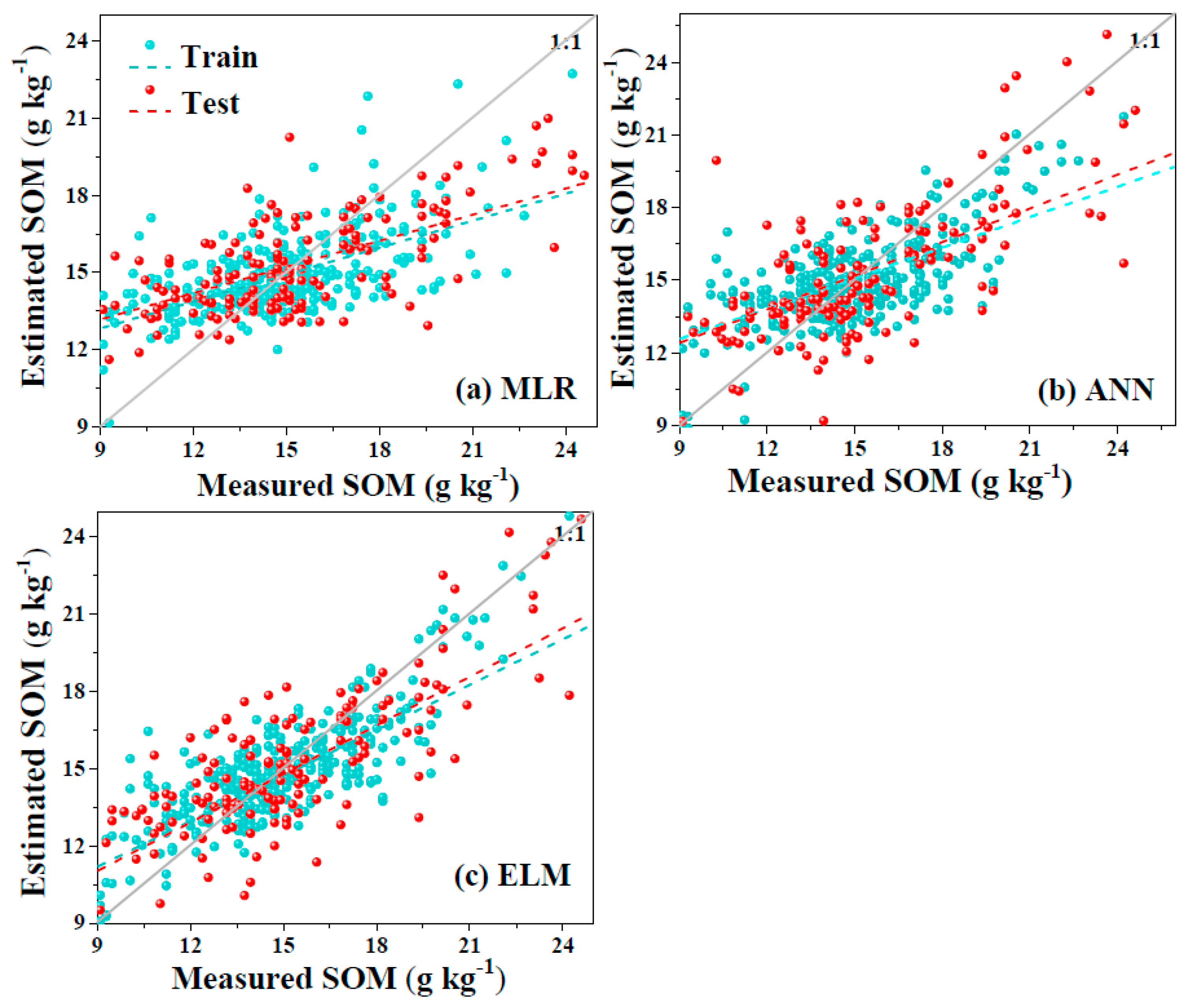
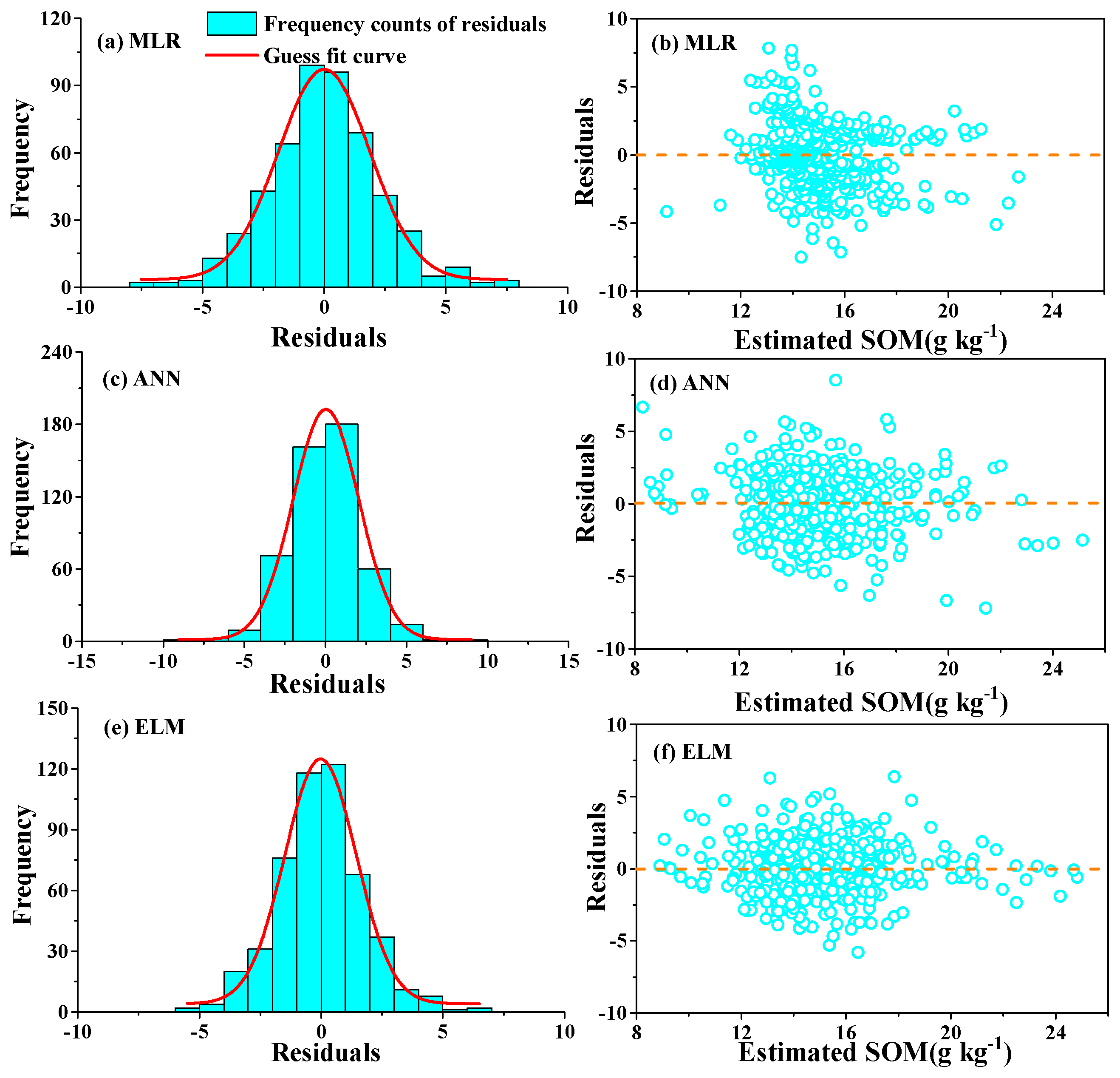
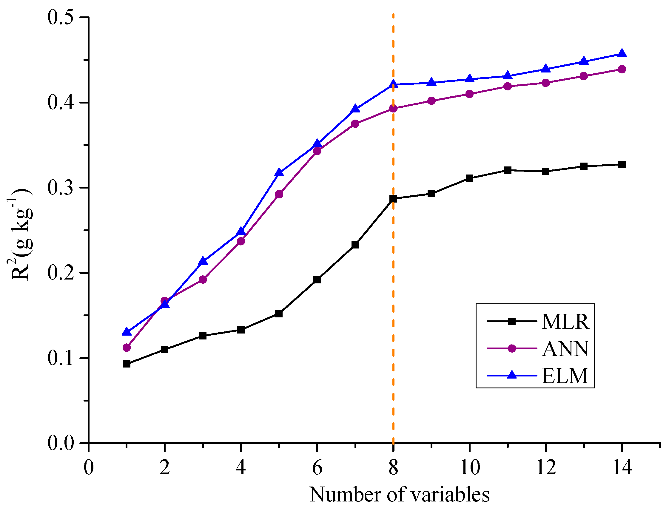
3.3. Prediction of SOM Content by MLR, ANN and ELM Models

An MLR model was derived to predict the SOM content using three PCs, which are the principal components converted from the auxiliary variables. As can be seen in

Table 3. Assessment of the MLR for predicting SOM content by PCs.

	Training Data Set			Testing Data Set			D-W a
	ME (g kg−1)	RMSE (g kg−1)	R2	ME (g kg−1)	RMSE (g kg−1)	R2
MLR	11.32	2.19	0.317	12.53	2.25	0.292	1.651

^a Durbin-Watson statistics.

, the determination coefficients (R²) of the MLR for both the training data set and the test data set were 0.317 and 0.292, respectively, which showed the barely satisfactory effect of linear fitting and indicated the complex variability between the SOM content and the multi-source factors.

SOM = 0.2582 − 0.5979 × PC1 + 0.3076 × PC2 + 0.0781 × PC3

For ANN and ELM, all the PCs were used as input variables. In order to demonstrate the practical use of the ELM as an efficient learning prediction method, the data set was divided into two independent groups (training data set included 330 samples and testing data set included 142 samples) and simultaneously controlled the hidden-layer nodes to avoid the over-fitting of the optimal unbiased estimation. In fact, the implementation of ELM should achieve a balance between the precision and simplification of the model parameters, which adjusted the neuron numbers. The derived accuracy of the ANN and ELM models from the ME values displayed a stable precision and small overestimation with six PCs, and between 18 and 30 neurons. The results revealed that the optimized ANN and ELM network architectures were 3-26-1 and 3-23-1 with the sigmoid kernel function, respectively, indicating that there were three input nodes in the input layer, 23 hidden-layer nodes, and one output-layer node, as shown in

Table 4. Parameters and evaluation statistics for the most significant ANN and ELM models.

Methods	Selected Architecture a	Training Data Set			Testing Data Set			Run Time (s)
		ME (g kg−1)	RMSE (g kg−1)	R2	ME (g kg−1)	RMSE (g kg−1)	R2
ANN	3-26-1	9.04	1.766	0.476	8.56	1.692	0.491	52
ELM	3-23-1	7.16	1.618	0.561	6.93	1.531	0.583	160

^a Number of the nodes in input layer, hidden layer, and output layer, respectively.

. For the best ELM model, the values of ME and RMSE were 6.93 g kg⁻¹ and 1.531 g kg⁻¹, respectively, for the SOM content. Compared with the MLR and ANN model, the ELM had larger R² and lower RMSE values, which could explain 58.3% of the variances in the SOM. More importantly, the run time of the ELM model was faster than ANN, which exhibited an efficient analytic ability between the correlative factors and SOM content. The prediction performance of ELM was comparable to, but better than, the regression and ANN reported by Li et al. (2010) [28] and Mirzaee et al. (2016) [13].

The residuals were obtained using the difference between the measured SOM data and the results of the MLR, ANN, and ELM prediction data. As can be seen in the estimated values of the SOM content, which were plotted against the measured values for the training sites and validation sites (Figure 2), the scatter plots of the ELM model displayed a better compactness and fewer outliers in comparison with the other methods. To further analyze the model performance by the relationship between the residuals and predicted SOM, a histogram of the residuals, a Gauss fitting curve, and the residuals versus the estimated SOM content were plotted in Figure 3. The result of the Kolmogorov-Smirnov (K-S) test showed that the distribution of residuals had a good fit with a normal distribution, which was 0.42, 0.37, and 0.32 in the MLR, ANN, and selected ELM models, respectively. Additionally, the graph also indicates that the residuals randomly display isotropic characteristics around zero (0). Furthermore, it is essential to perform an analysis of the distribution of residuals, because it was directly used to calculate the experimental semivariograms for the spatial autocorrelation of kriging interpolation.

3.4. Spatial Prediction of SOM Content by Geostatistical Methods

As shown in

Table 5. Semivariogram model parameters for SOM content and residuals of MLR, ANN, and ELM.

Variogram	Model	Range (km)	Nugget	Sill	Nugget/Sill
Semivariograms of SOM	Exponential	4.57	0.031	0.115	0.270
Residuals of MLR	Exponential	3.34	0.345	0.979	0.352
Residuals of ANN	Exponential	3.60	0.503	1.166	0.431
Residuals of ELM	Exponential	3.06	0.478	1.213	0.394

, the best-fit parameters of OK determined the various semivariograms and spatial dependence of the residuals for the SOM content. The nugget/sill ratio, namely the nugget effect (NE), was used to describe the degree of spatial dependence and random variation for the SOM content, and was divided into a strong spatial correlation (NE ≤ 25%), moderate spatial dependence (25% < NE ≤ 75%), and weak spatial dependence (NE > 75%). Additionally, interpolation methods, including ordinary kriging, residuals kriging of regression, residuals kriging of ANN, and residuals kriging of ELM, were conducted to predict the SOM content in the study area. The NE of this study showed that all methods had a moderate spatial dependence.

Table 6. Accuracy assessment statistics for interpolation methods at the test sites.

Interpolation Methods	ME (g kg−1)	RMSE (g kg−1)	R2	RPD
SK	15.95	3.26	0.192	0.88
OK	11.05	2.071	0.363	1.39
ROK	9.97	1.974	0.422	1.45
ANNOK	6.22	1.463	0.611	1.96
ELMOK	5.37	1.402	0.671	2.05

shows the statistical results of the geostatistical methods in the test data set, and the OK approach illustrates a better performance for the production of SOM content in comparison with simple kriging (SK).

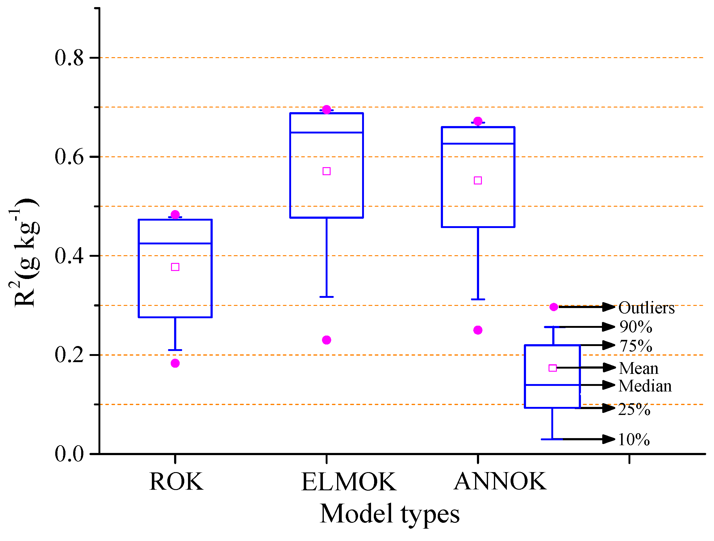
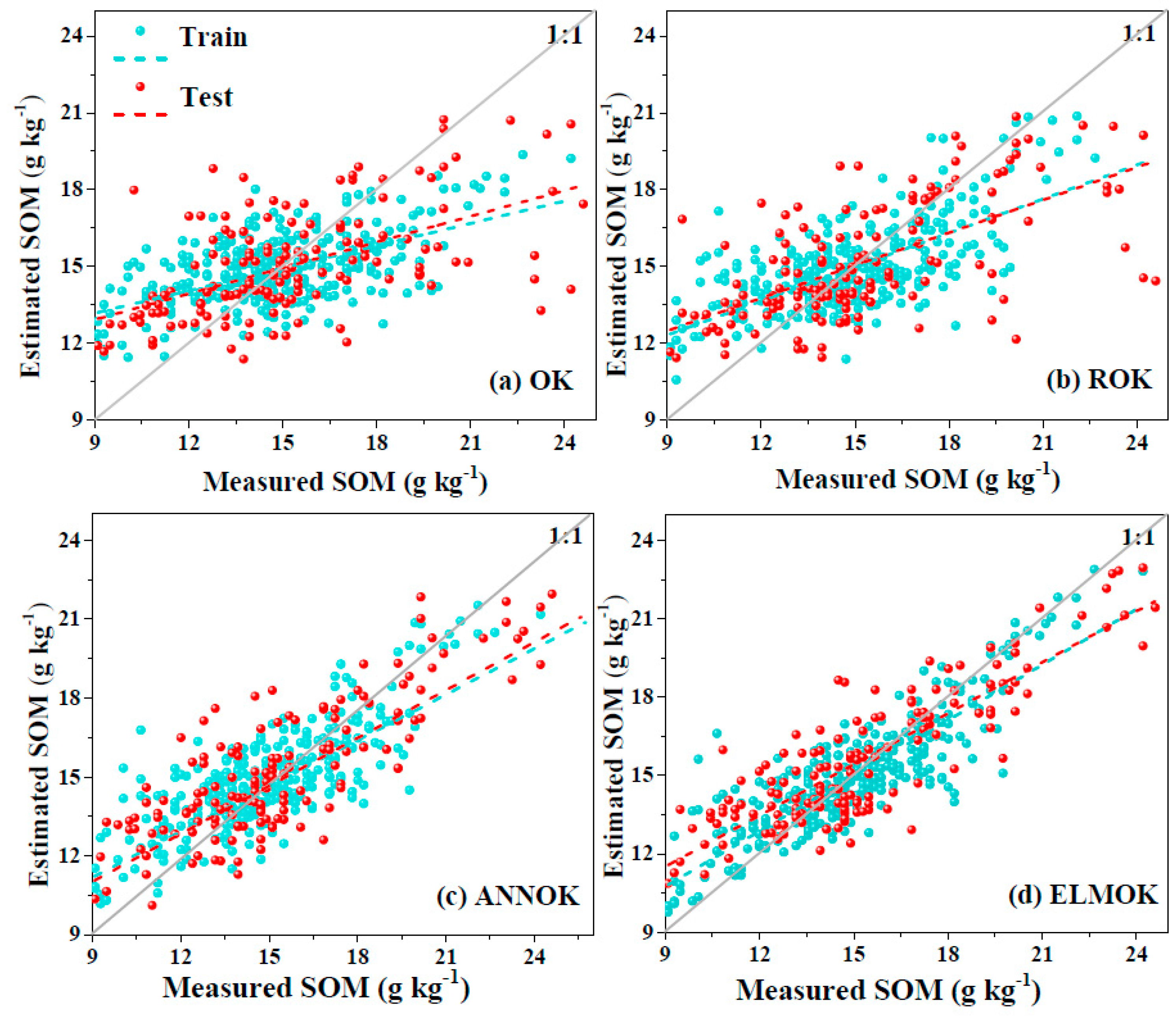
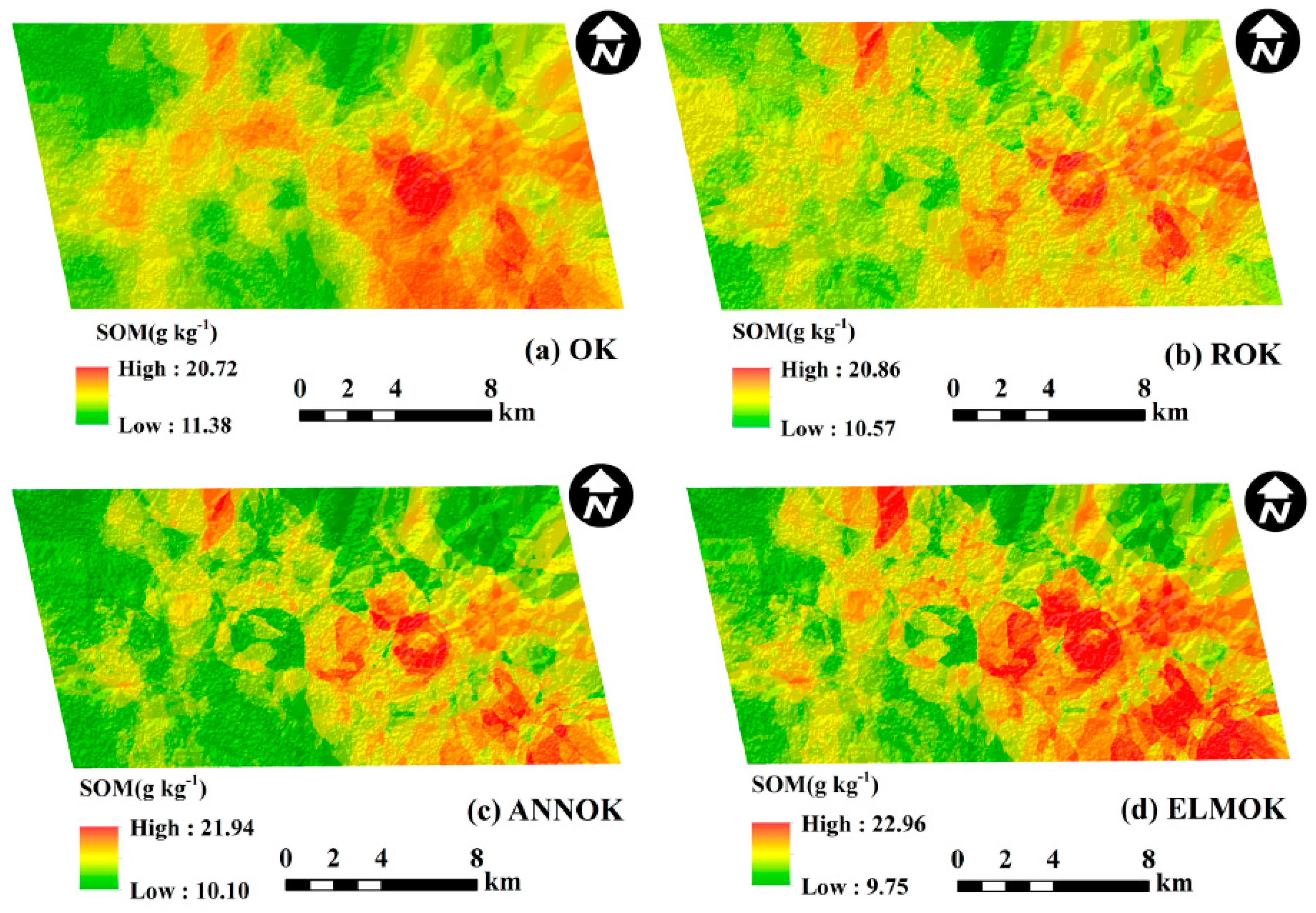
3.5. Spatial Prediction of SOM Content by Hybrid Geostatistical Methods

According to Equation (10), the hybrid geostatistical methods of MLROK, ANNOK, and ELMOK were used to implement the prediction of SOM content. As shown in Table 6, the ELM-kriging approach had a lower RMSE (1.402 g kg⁻¹) and a high R² (0.671) for the prediction of the SOM content in comparison with the geostatistical methods, and the ratio of performance to deviation (RPD) was 2.05. Figure 4 shows the estimated values of the SOM content, which were plotted against the measured values for the training sites and test sites. The scatter plots of the ELMOK model exhibits less outliers and a better compactness in comparison with the other models. In short, ELM-kriging obtains a better estimation accuracy of the SOM content than the other methods. As can be shown in Figure 5, these four prediction methods had a similar distribution trend of the SOM content in the general spatial patterns, and the main concentration of high SOM values was in the southeast of the study area. However, transitions among the spatial heterogeneity of local SOM had better gradients in the prediction maps produced by ELMOK than by the other methods. In addition, the ranges of the SOM content (both the lower values and the higher values) in the estimated maps by ELMOK were much closer to the measured values, which had a deeper nonlinear analytic ability for SOM.

4. Discussion

4.1. Driving Force Analysis of Auxiliary Variables for SOM

In order to further determine the driving forces of multi-source auxiliary variables, we observed the effects of different factors for the spatial variability of soil organic matter by adding or deleting collaborative variables, which was based on the idea of the stepwise regression in MLR, ANN, and ELM prediction models. By adding or removing the amounts of variables (the type of each variable to be added or deleted should be the same in the three models), we obtained the variation trend of the coefficient of determination (R²) of the three models from one to 14 variables, and then drew the distribution box diagram according to the coefficient of each model. As can be seen in Figure 6 and Figure 7, according to the R² of each model with a different number of variables, the interpretative ability of three models for SOM content from better to worse were: ELM > ANN > MLR. When the number of variables was less than eight, the R² showed obvious attenuation. However, when the number of variables gradually increased from 8 to 14, the R² of the three models did not significantly improve. In addition, the mean value of R² between the auxiliary variables and soil organic matter in the three models in descending order were: ELMOK > ANNOK > ROK.

Based on the result of the driving force analysis of the auxiliary variables, the TMEAN, ELE, B4, and NDVI factors had the greatest influence on the spatial variability of SOM, which were not only consistent with its impact on global change, but also reflected the significant responding relationship between soil organic matter and global change. Furthermore, the analysis result of the remote sensing variables was similar to the report of Mirzaee et al. (2016), in which B4 and NDVI had a greater influence on the spatial variability of soil organic matter. This may be due to vegetation and organic matter containing a major carbon source, thus forming a potential strong correlation and driving force. As a result, there is a significant multi-dimensional hierarchy relationship between the environmental variables and remote sensing data, and the more types of the variables there are, the more obvious nonlinear relationship between the SOM and auxiliary variables is.

4.2. Sustainable Monitoring of Digital Mapping for SOM

The estimated results of the SOM content by ELMOK were much closer to the measured values, which were demonstrated an acceptable range for monitoring site-specific SOM and its quality evaluation in comparison with [8,13,14]. Generally, a higher resolution and higher precision of SOM can capture its changes more acutely in a regional spatial range, while it is difficult to reflect the continuous dynamic changes because only one year of data is used. However, there is not a unified standard for the sustainable monitoring of SOM, so how can we understand and realize its sustaining value? The sustainable monitoring of SOM can be defined using two aspects: Firstly, in the vertical aspect (sustainable monitoring of time series of data driven), the ELM model can be used in the sustainable prediction for SOM, which overcomes the interference of sample density and multi-collinearity among auxiliary variables. Simultaneously, the ELM has the capability to auto-analyze the nonlinear relationships between multi-source auxiliary variables and SOM by self-learning. Secondly, in the horizontal aspect (sustainable monitoring of special non-point), the integration of ELM and kriging can realize the special sustainability of SOM monitoring in a site-specific prediction, which includes the continuous distribution of SOM and the monitoring of variability. There are several possible routes which can be followed for the sustainable monitoring of SOM based on a revisit sampling period and method design.

(1) The sustainable monitoring of SOM includes the continuity of spatial variation and time series. It is difficult to collect samples by an accurate point-to-point method in future years and for the same study area. Perform pixel-based revisit sampling is an effective procedure. On the one hand, for auxiliary variables, it is easy to obtain the values of pixels which correspond with the sampling points; On the other hand, for the digital mapping, it is practical to use the range of pixels instead of the sampling point location, because the specific resolution of the non-point source of SOM is the ultimate objective in different scales. Using the pre-existing mapping results of SOM as the basic map of sampling design, the SOM content using the auxiliary variables can be predicted several years later, which will reduce the quantity of sampling points and reduce both the cost and time.

(2) Perform the integrated approach, which included the hybrid geostatistical method and spatial downscaling based on ensemble learning thinking [47]. The integrated approach realized the win-win relationships, which not only absorbed the advantages of the machine learning-kriging method such as a high efficiency, high accuracy, and geostatistical significance, but also combined the advantages of the spatial downscaling approach, such as an easy availability, spatial variation, and adaptation of multi-scale.

(3) Perform a deep analysis for the mapping results of SOM in different years. It is essential to capture the regional changes which became observably high or low for the SOM content from the mapping results in different years. There may be some reasons which caused this change, such as the cropping system, soil type, auxiliary variables, and so on. Furthermore, the sustainability of spatial and temporal monitoring of SOM should have a closer relationship with soil health and climate change.

5. Conclusions

In this study, an extreme learning machine approach was used to predict the spatial distribution of SOM content with multi-source auxiliary variables of remote sensing, topographic, climate, and soil properties at a regional scale. A two-stage integrated process was proposed that incorporated an ELM model with residual estimation by ordinary kriging, which was compared to the interpolation methods of ANNOK and ROK for assessing its feasibility, efficiency, and prediction accuracy. The results indicated that the prediction accuracy of SOM content was raised by ELMOK, with a lower RMSE value (1.402 g kg⁻¹) and higher R² (0.671) in comparison with the other methods. Additionally, a driving force analysis of the auxiliary variables identified TMEAN, ELE, B4, and NDVI as the most important factors affecting the spatial variability of SOM. This finding could prove a deeper driven significance for the nonlinear and multi-dimensional hierarchy relationship between auxiliary variables and SOM, and gave preference to select the optimized feature factors in similar areas. More importantly, for the sustainable monitoring of SOM, there are several possible routes that are based on pixel-based revisit sampling, an integrated approach of the hybrid geostatistical method, and spatial downscaling so that they are adapted to the different scales, and which analyze the changes of mapping results of SOM in time series. The proposed ELM-ordinary kriging methodology is a promising and efficient approach for predicting the spatial variability of SOM at a regional scale.

References

1. Manlay, R.; Feller, C.; Swift, M. Historical evolution of soil organic matter concepts and their relationships with the fertility and sustainability of cropping systems. Agric. Ecosyst. Environ. 2007, 119, 217–233. [Google Scholar] [CrossRef]
2. Brantley, S.L. Understanding soil time. Science 2008, 321, 1454–1455. [Google Scholar] [CrossRef] [PubMed]
3. Lehmann, J.; Kleber, M. The contentious nature of soil organic matter. Nature 2015, 528, 60–68. [Google Scholar] [CrossRef] [PubMed]
4. Zhao, Y.N.; He, X.H.; Huang, X.C.; Zhang, Y.Q.; Shi, X.J. Increasing soil organic matter enhances inherent soil productivity while offsetting fertilization effect under a rice cropping system. Sustainability 2016, 8, 879. [Google Scholar] [CrossRef]
5. Jeffrey, D.S. Sustainable Development. Science 2004, 304, 649. [Google Scholar]
6. Durigan, M.R.; Cherubin, M.R.; de Camargo, P.B.; Ferreira, J.N.; Berenguer, E.; Gardner, T.A.; Barlow, J.; Dias, C.T.D.S.; Signor, D.; Junior, R.C.D.O.; et al. Soil Organic Matter Responses to Anthropogenic Forest Disturbance and Land Use Change in the Eastern Brazilian Amazon. Sustainability 2017, 9, 379. [Google Scholar] [CrossRef]
7. Sanchez, P.A.; Ahamed, S.; Carré, F.; Hartemink, A.E.; Hempel, J.; Huising, J.; Lagacherie, P.; Mcbratney, A.B.; Mckenzie, N.J.; Santos, M.L.D.M.; et al. Digital soil map of the world. Science 2009, 325, 680–681. [Google Scholar] [CrossRef] [PubMed]
8. Guo, P.T.; Li, M.F.; Luo, W.; Tang, Q.F.; Liu, Z.W.; Lin, Z.M. Digital mapping of soil organic matter for rubber plantation at regional scale: An application of random forest plus residuals kriging approach. Geoderma 2015, 237–238, 49–59. [Google Scholar] [CrossRef]
9. Meersmans, J.; Van Wesemael, B.; Goidts, E.; Van Molle, M.; De Baets, S.; De Ridder, F. Spatial analysis of soil organic carbon evolution in Belgian croplands and grasslands, 1960–2006. Glob. Chang. Biol. 2011, 17, 466–479. [Google Scholar] [CrossRef]
10. Zhang, S.; Huang, Y.; Shen, C.; Ye, H.; Du, Y. Spatial prediction of soil organic matter using terrain indices and categorical variables as auxiliary information. Geoderma 2012, 171, 35–43. [Google Scholar] [CrossRef]
11. Piccini, C.; Marchetti, A.; Francaviglia, R. Estimation of soil organic matter by geostatistical methods: Use of auxiliary information in agricultural and environmental assessment. Ecol. Indic. 2014, 36, 301–314. [Google Scholar] [CrossRef]
12. Feng, C.; Kissel, D.E.; West, L.T.; Adkins, W. Field-scale mapping of surface soil organic carbon using remotely sensed imagery. Soil Sci. Soc. Am. J. 2000, 64, 746–753. [Google Scholar]
13. Mirzaee, S.; Ghorbani-Dashtaki, S.; Mohammadi, J.; Asadi, H.; Asadzadeh, F. Spatial variability of soil organic matter using remote sensing data. Catena 2016, 145, 118–127. [Google Scholar] [CrossRef]
14. Dai, F.; Zhou, Q.; Lv, Z.; Wang, X.; Liu, G. Spatial prediction of soil organic matter content integrating artificial neural network and ordinary kriging in Tibetan Plateau. Ecol. Indic. 2014, 45, 184–194. [Google Scholar] [CrossRef]
15. Zhang, R.; Shouse, P.; Yates, S. Use of pseudo-crossvariograms and cokriging to improve estimates of soil solute concentrations. Soil Sci. Soc. Am. J. 1997, 61, 0361–5995. [Google Scholar] [CrossRef]
16. Triantafilis, J.; Odeh, I.O.A.; Mcbratney, A.B. Five Geostatistical Models to Predict soil salinity from electromagnetic induction data across irrigated cotton. Soil Sci. Soc. Am. J. 2001, 65, 869–878. [Google Scholar] [CrossRef]
17. Lark, R.M. Robust estimation of the pseudo cross-variogram for cokriging soil properties. Eur. J. Soil Sci. 2002, 53, 253–270. [Google Scholar] [CrossRef]
18. Wu, C.F.; Wu, J.P.; Luo, Y.M.; Zhang, L.M.; Degloria, S.D. Spatial prediction of soil organic matter content using cokriging with remotely sensed data. Soil Sci. Soc. Am. J. 2009, 73, 1202–1208. [Google Scholar] [CrossRef]
19. Mishra, U.; Lal, R.; Liu, D.S.; Meirvenne, M.V. Predicting the spatial variation of the soil organic carbon pool at a regional scale. Soil Sci. Soc. Am. J. 2010, 74, 906–914. [Google Scholar] [CrossRef]
20. Marchetti, A.; Piccini, C.; Francaviglia, R.; Mabit, L. Spatial distribution of soil organic matter using geostatistics: A key indicator to assess soil degradation status in central Italy. Pedosphere 2012, 22, 230–242. [Google Scholar] [CrossRef]
21. Hengl, T.; Heuvelink, G.B.M.; Rossiter, D.G. About regression-kriging: From equations to case studies. Comput. Geosci. 2007, 33, 1301–1315. [Google Scholar] [CrossRef]
22. Zhao, Z.; Chow, T.L.; Rees, H.W.; Qi, Y.; Xing, Z.; Meng, F.R. Predict soil texture distributions using an artificial neural network model. Comput. Electron. Agric. 2009, 65, 36–48. [Google Scholar] [CrossRef]
23. Cheng, X.F.; Shi, X.Z.; Yu, D.S.; Pan, X.Z.; Wang, H.J.; Sun, W.X. Using GIS spatial distribution to predict soil organic carbon in subtropical China. Pedosphere 2004, 14, 425–431. [Google Scholar]
24. Odeha, I.O.A.; Mcbratney, A.B.; Chittleborough, D.J. Spatial prediction of soil properties from landform attributes derived from a digital elevation model. Geoderma 1994, 63, 197–214. [Google Scholar] [CrossRef]
25. Kumar, S.; Lal, R.; Liu, D. A geographically weighted regression kriging approach for mapping soil organic carbon stock. Geoderma 2012, 189–190, 627–634. [Google Scholar] [CrossRef]
26. Yang, Q.Y.; Jiang, Z.C.; Li, W.J.; Li, H. Prediction of soil organic matter in peak-cluster depression region using kriging and terrain indices. Soil Tillage Res. 2014, 144, 126–132. [Google Scholar] [CrossRef]
27. Knotters, M.; Brus, D.J.; Voshaar, J.H.O. A comparison of kriging, co-kriging and kriging combined with regression for spatial interpolation of horizon depth with censored observations. Geoderma 1995, 67, 227–246. [Google Scholar] [CrossRef]
28. Li, Y. Can the spatial prediction of soil organic matter contents at various sampling scales be improved by using regression kriging with auxiliary information? Geoderma 2010, 159, 63–75. [Google Scholar] [CrossRef]
29. Somaratne, S.; Seneviratne, G.; Coomaraswamy, U. Prediction of soil organic carbon across different land-use patterns. Soil Sci. Soc. Am. J. 2005, 69, 1580–1589. [Google Scholar] [CrossRef]
30. Zhao, Z.Y. Using artificial neural network models to produce soil organic carbon content distribution maps across landscapes. Can. J. Soil Sci. 2010, 90, 75–87. [Google Scholar] [CrossRef]
31. Li, Q.Q.; Yue, T.X.; Wang, C.Q.; Zhang, W.J.; Yu, Y.; Li, B. Spatially distributed modeling of soil organic matter across China: An application of artificial neural network approach. Catena 2013, 104, 210–218. [Google Scholar] [CrossRef]
32. Huang, G.B.; Zhu, Q.Y.; Siew, C.K. Extreme learning machine: A new learning scheme of feedforward neural networks. IEEE Int. Jt. Conf. Neural Netw. 2004, 2, 985–990. [Google Scholar]
33. Huang, G.; Huang, G.B.; Song, S.; You, K. Trends in extreme learning machines: A review. Neural Netw. 2014, 61, 32–48. [Google Scholar] [CrossRef] [PubMed]
34. Ding, S.; Zhao, H.; Zhang, Y.; Xu, X.; Nie, R. Extreme learning machine: Algorithm, theory and applications. Artif. Intell. Rev. 2013, 44, 103–115. [Google Scholar] [CrossRef]
35. Liu, X.; Lin, S.; Fang, J.; Xu, Z. Is extreme learning machine feasible? A theoretical assessment (Part II). IEEE Trans. Neural Netw. Learn. Syst. 2014, 26, 7–20. [Google Scholar] [CrossRef] [PubMed]
36. Deng, C.W.; Huang, G.B.; Jia, X.U.; Tang, J.X. Extreme learning machines: New trends and applications. Sci. China Inf. Sci. 2015, 58, 1–16. [Google Scholar] [CrossRef]
37. The Ministry of Agriculture of the People’s Republic of China. Rules for Soil Quality Survey and Assessment (NY/T 1634-2008). 2008. Available online: http://www.moa.gov.cn/ (accessed on 5 November 2016). (In Chinese)
38. The Ministry of Agriculture of the People’s Republic of China. Chinese Agriculture Industry Standard (NY/T 1211.1-2006). 2006. Available online: http://www.moa.gov.cn/ (accessed on 5 November 2016). (In Chinese)
39. Read, J.W.; Ridgell, R.H. On the use of the conventional carbon factor in estimating soil organic matter. Soil Sci. 1922, 13, 1–6. [Google Scholar] [CrossRef]
40. Nelson, D.W.; Sommers, L.E. A rapid and accurate method for estimating organic carbon in the soil. Proc. Indiana Acad. Sci. 1975, 84, 456–462. [Google Scholar]
41. The National Aeronautics and Space Agency (NASA). Available online: http://landsat.usgs.gov/ (accessed on 1 December 2016).
42. Huete, A.R.; Liu, H.Q. An error and sensitivity analysis of the atmospheric- and soil-correcting variants of the NDVI for the MODIS-EOS. IEEE Trans. Geosci. Remote Sens. 1994, 32, 897–905. [Google Scholar] [CrossRef]
43. International Scientific & Technical Data Mirror Site, Computer Network Information Center, Chinese Academy of Sciences. Available online: http://www.gscloud.cn/ (accessed on 2 December 2016). (In Chinese).
44. Zhang, B.C.; Zhang, Y.M.; Zhao, J.C.; Wu, N.; Chen, R.Y.; Zhang, J. Microalgal species variation at different successional stages in biological soil crusts of the Gurbantunggut Desert, Northwestern China. Biol. Fertil. Soils 2009, 45, 539–547. [Google Scholar] [CrossRef]
45. Pirie, A.; Singh, B.; Islam, K. Ultra-violet, visible, near-infrared, and mid-infrared diffuse reflectance spectroscopic techniques to predict several soil properties. Soil Res. 2005, 43, 713–721. [Google Scholar] [CrossRef]
46. Razakamanarivo, R.H.; Grinand, C.; Razafindrakoto, M.A.; Bernoux, M.; Albrecht, A. Mapping organic carbon stocks in eucalyptus plantations of the central highlands of Madagascar: A multiple regression approach. Geoderma 2011, 162, 335–346. [Google Scholar] [CrossRef]
47. Malone, B.P.; Styc, Q.; Minasny, B.; Mcbratney, A.B. Digital soil mapping of soil carbon at the farm scale: A spatial downscaling approach in consideration of measured and uncertain data. Geoderma 2017, 290, 91–99. [Google Scholar] [CrossRef]
Figure 1. Location of the study area in central China and the distribution of the training and validation sites.
Sustainability 09 00754 g001
Figure 2. Observed versus estimated SOM content, using (a) MLR, (b) ANN, and (c) ELM models.
Sustainability 09 00754 g002
Figure 3. MLR, ANN, and ELM diagnostics of the residuals: histogram ((a) MLR model, (c) ANN model, and (e) ELM model) and residuals versus estimated SOM value ((b) MLR model, (d) ANN model, and (f) EKM model).
Sustainability 09 00754 g003
Figure 4. Observed versus estimated SOM content, using (a) OK, (b) ROK, (c) ANNOK, and (d) ELMOK models.
Sustainability 09 00754 g004
Figure 5. Predicted SOM content (g kg−1) maps by (a) OK, (b) ROK, (c) ANNOK, and (d) ELMOK, all the maps are in 30 m resolution.
Sustainability 09 00754 g005
Figure 6. Driving force analysis of auxiliary variables for SOM by MLR, ANN, and ELM.
Sustainability 09 00754 g006
Figure 7. The box graph of different model types by ROK, ANNOK, and ELMOK.
Sustainability 09 00754 g007