
Coordinated Optimal Operation Method of the Regional Energy Internet

Abstract
:1. Introduction
2. Structure and Energy Flow Characteristics of Regional Energy Internet
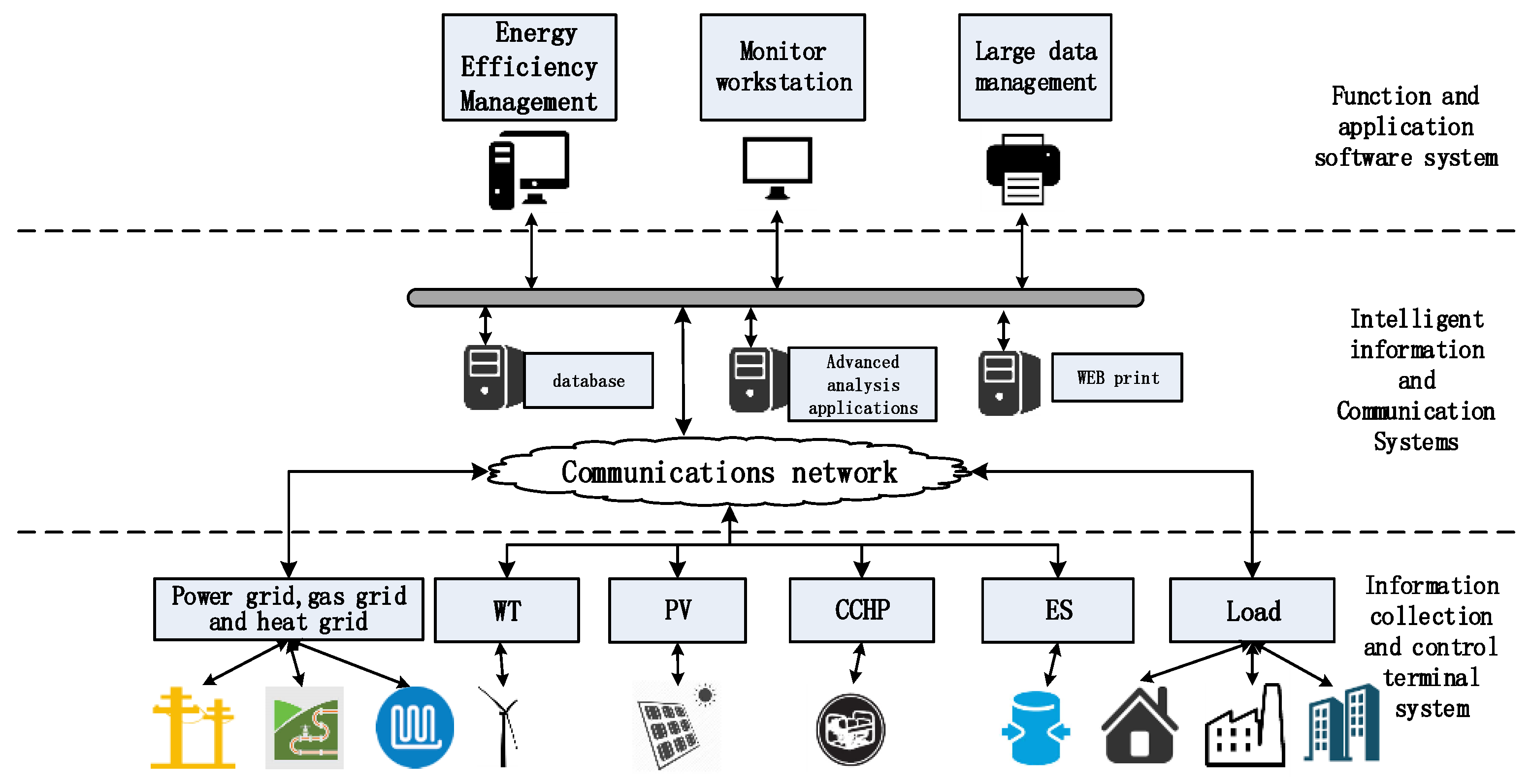
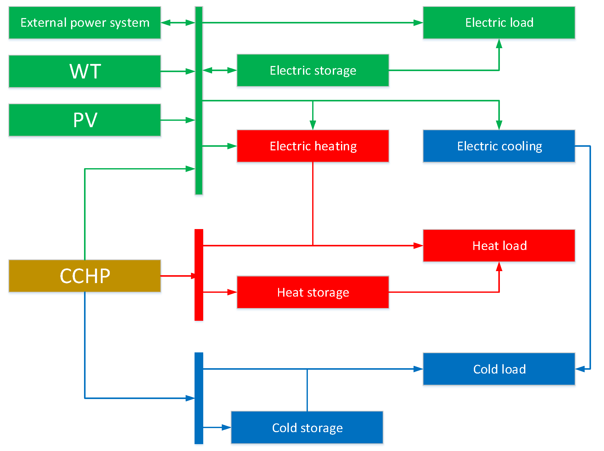
Structure
- (1)
- The regional EI is an organic whole combined by a power grid, a thermal network, a gas network, a regional distributed energy station and an operation center;
- (2)
- There is a variety of energy devices in the region, such as WT, PV, CCHP units, and ES equipment (including electric storage, heat storage and cold storage), to achieve a variety of energy complements;
- (3)
- There is a wide variety of loads in addition to electric load, including heat and cold load;
- (4)
- Information flow and energy flow are more closely linked and complex.
3. Coordinated Optimal Operation Model
3.1. Power Output Model and Cost Model
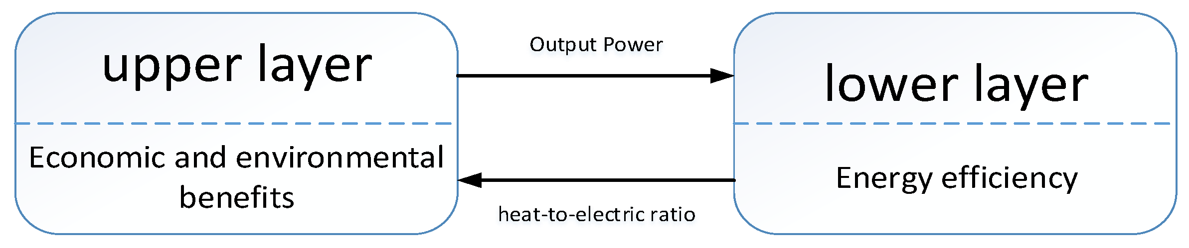
3.2. Two-Layer Optimization Objective Function
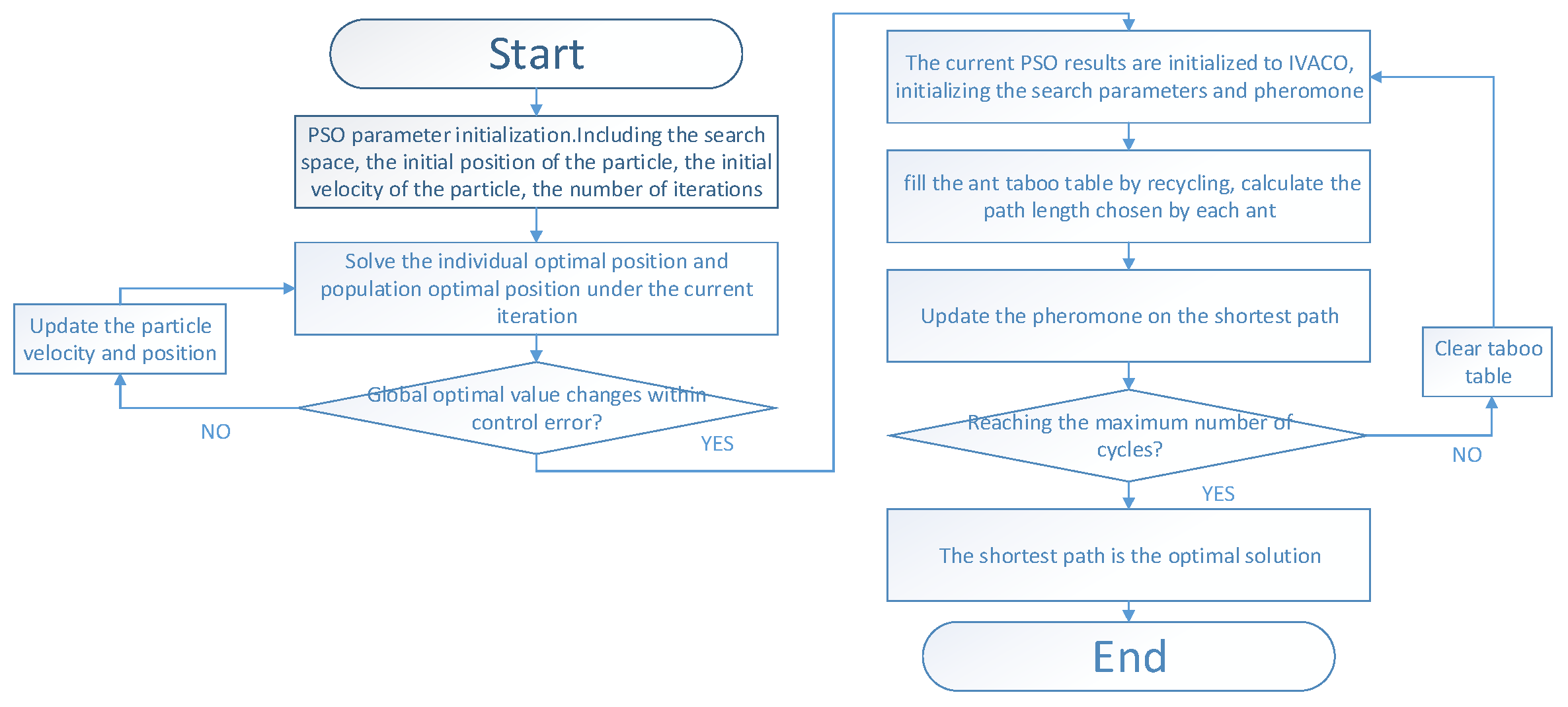
3.3. Solving Algorithm
- (1)
- Input power matrix of load, PV, WT, and other constants. The results of the optimal scheduling at t-1 are taken as the initial value variables at t (if t = 0, then the initial value takes the last time in the previous day);
- (2)
- PSO is used to solve iteratively. Calculate the lower target first, obtain the position and velocity of the particles, and feed back to the upper layer. Then, calculate the upper target, update the velocity and position, and feed back to the lower layer. After each iteration, perform a power flow calculation to check whether the stability constraint is met. If it is not satisfied, return to the first step, adjust the initial value. If satisfied, carry on to the next step;
- (3)
- Repeat iterations until the objective function value changes within the control range;
- (4)
- The optimized variable results from (2) are taken as the initial value of the IVACO iteration. Calculate by following the steps above; then, output the final result.
4. Case Study
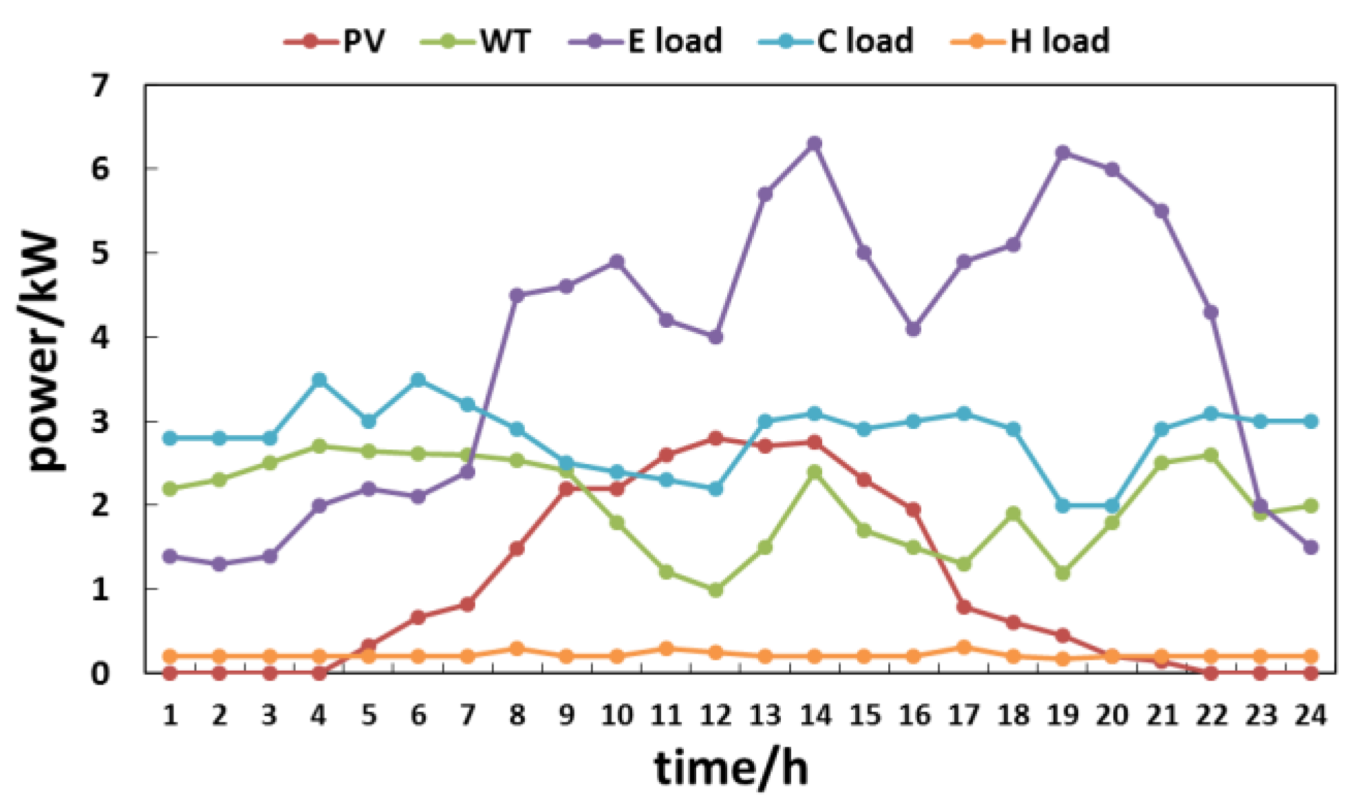
4.1. Basic Data
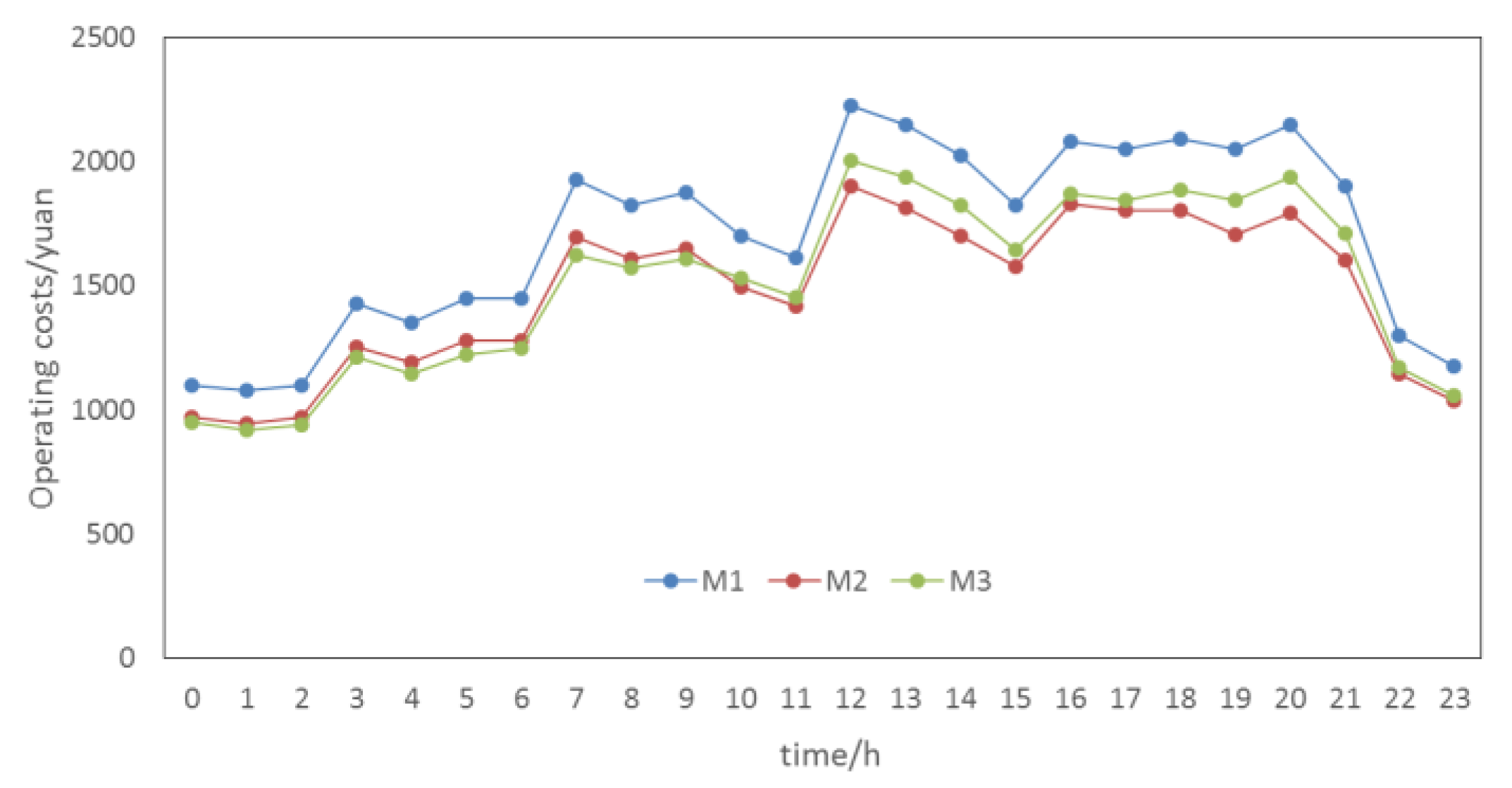
- Mode 1 (M1): In this situation, the CCHP unit adopts a constant HTER to supply the electric energy and heat/cold energy;
- Mode 2 (M2): The model proposed in this paper. The CCHP unit adopts an adjustable HTER.
- Mode 3 (M3): On the basis of M2, the ES operating cost is not included in the objective function, only taking into account its operational constraints.
4.2. Simulation Results
- (1)
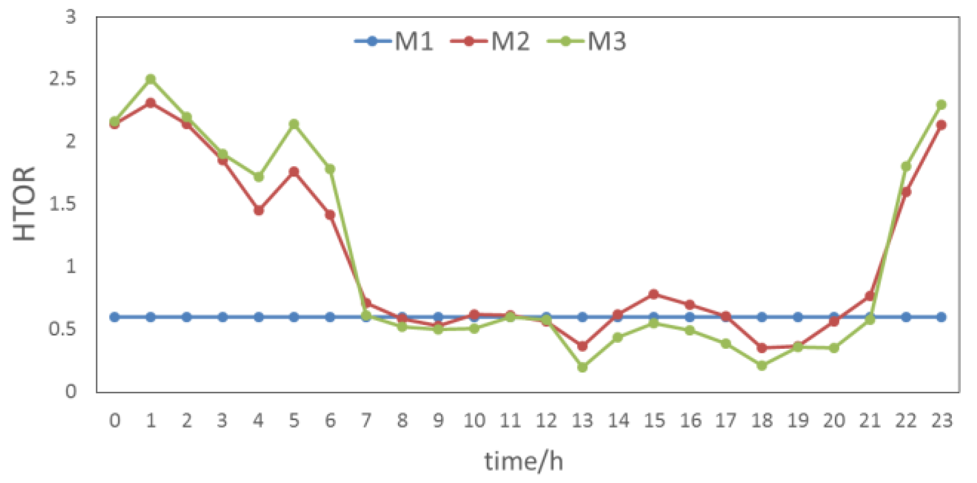
- It can be seen from Figure 6 that the optimal HTER at each time is affected by the change of the heat–electric load ratio in the EI. This shows that the optimal HTER is related to the load distribution in the region.
- (2)
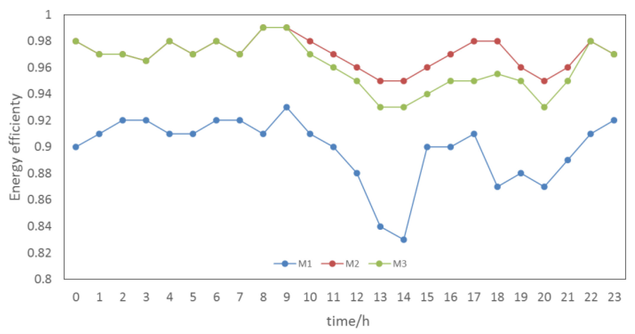
- From Figure 7 and Figure 8, and Table 2, we can determine that in the case of adjustable HTER, the CCHP unit enhances the heat power output limit, which leads to an increase in the output of the CCHP unit in the source; its operation cost and energy efficiency have improved compared with the direct use of boiler heating.
- (3)
- From Figure 6, Figure 7 and Figure 8, it can be found that there is a certain positive correlation between the optimal HTER and the energy efficiency, and there is a certain inverse correlation with the operation cost. When the HTER is relatively high, the energy efficiency is high and the cost is also lower. It can be concluded that by further analysis, the HTER and efficiency exist in two valley areas, namely 13:00–14:00 and 18:00–19:00. These two periods are the electric peak periods; the electric power output is high, affecting the CCHP unit thermoelectric balance ratio.
- (4)
- The load situation has a greater impact on the operation of the EI. When the load is large, the economy and energy efficiency of the EI will be affected. Therefore, it is effective to improve the comprehensive benefit of the EI by a demand response strategy to reduce the peak and valley difference of the load.
- (5)
- From some of the calculation results (e.g., 09:00 and 14:00), energy efficiency and economic cost are not achieving the best results simultaneously. This is due to the two-layer objective function of this paper. However, from a longer time scale, the model proposed in this paper strikes a reasonable balance between economic cost and energy efficiency, so that the calculation result of the whole day is satisfactory.
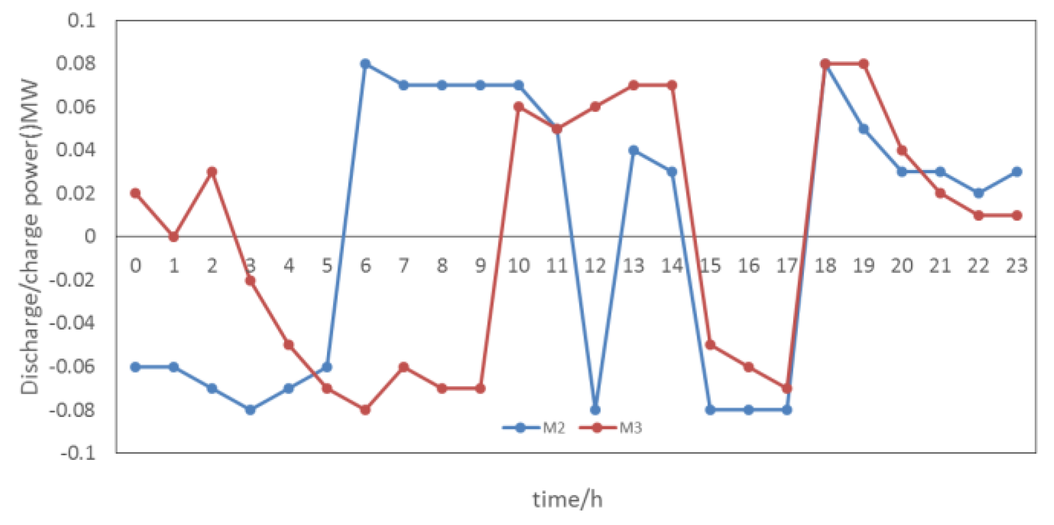
- (1)
- The output changes in M2 are more stable, and the charge/discharge interval is more stable and works more efficiently. This can extend its life expectancy, which also can be seen from Table 2, (the cost of ES is lower in M2);
- (2)
- The ES strategy and real-time electricity price are more closely aligned in M2. ES discharges in the peak price and charges in the valley price. This maximization of the benefits reduces the overall operating costs;
- (3)
- Finally, a reasonable charge/discharge of ES will ease the CCHP unit’s output pressure, and optimize its operation, resulting in an improvement in energy efficiency.
5. Conclusions
- (1)
- Make appropriate simplifications for the optimal operation model of CCHP, and study the thermodynamic properties of the system to ensure that the optimization results will be closer to the actual project;
- (2)
- The operational state of the regional EI is complex and changeable, and there may be some deviation in the offline scheduling strategy, and further research on the online scheduling method is needed;
- (3)
- The proposed scheduling strategy can be used as a reference, which can be used to study the actual ES scheduling strategy.
Acknowledgments
Author Contributions
Conflicts of Interest
Appendix A

| Time | Price (yuan/kW·h) | Time | Price (yuan/kW·h) |
|---|---|---|---|
| 1 | 0.240 | 13 | 0.990 |
| 2 | 0.177 | 14 | 1.490 |
| 3 | 0.130 | 15 | 0.990 |
| 4 | 0.096 | 16 | 0.790 |
| 5 | 0.030 | 17 | 0.400 |
| 6 | 0.170 | 18 | 0.364 |
| 7 | 0.271 | 19 | 0.359 |
| 8 | 0.386 | 20 | 0.413 |
| 9 | 0.516 | 21 | 0.444 |
| 10 | 0.526 | 22 | 0.348 |
| 11 | 0.810 | 23 | 0.300 |
| 12 | 1.000 | 24 | 0.225 |
| Time | Price (yuan/kW·h) | Time | Price (yuan/kW·h) |
|---|---|---|---|
| 1 | 0.220 | 13 | 0.970 |
| 2 | 0.157 | 14 | 1.470 |
| 3 | 0.110 | 15 | 0.970 |
| 4 | 0.076 | 16 | 0.770 |
| 5 | 0.010 | 17 | 0.380 |
| 6 | 0.150 | 18 | 0.344 |
| 7 | 0.251 | 19 | 0.339 |
| 8 | 0.366 | 20 | 0.393 |
| 9 | 0.496 | 21 | 0.424 |
| 10 | 0.506 | 22 | 0.328 |
| 11 | 0.790 | 23 | 0.280 |
| 12 | 0.980 | 24 | 0.205 |
References
- Tian, S.M.; Luan, W.P.; Zhang, D.X.; Liang, C.H.; Sun, Y.J. Technical Forms and Key Technologies on Energy Internet. Proc. CSEE 2015, 35, 3482–3495. [Google Scholar]
- Lasseter, R.H. Microgrids and distributed generation. Intell. Autom. Soft Comput. 2010, 16, 225–234. [Google Scholar] [CrossRef]
- Chen, Q.X.; Liu, D.N.; Lin, J.; He, J.H.; Wang, Y. Business Models and Market Mechanisms of Energy Internet (1). Power Syst. Technol. 2015, 35, 3050–3056. [Google Scholar]
- Tseng, Y.C.; Lee, D.; Lin, C.F.; Chang, C.Y. The Energy Savings and Environmental Benefits for Small and Medium Enterprises by Cloud Energy Management System. Sustainability 2016, 8, 531. [Google Scholar] [CrossRef]
- Rifkin, J. The third industrial revolution. Eng. Technol. 2008, 3, 26–27. [Google Scholar] [CrossRef]
- Siano, P. Demand response and smart grids—A survey. Renew. Sustain. Energy Rev. 2014, 30, 461–478. [Google Scholar] [CrossRef]
- Pazouki, S.; Haghifam, M.; Moser, A. Uncertainty modeling in optimal operation of energy hub in presence of wind, storage and demand response. Int. J. Electr. Power Energy Syst. 2014, 61, 335–345. [Google Scholar] [CrossRef]
- Yang, F.; Bai, C.F.; Zhang, Y.B. Research on the value and implementation framework of energy internet. Proc. CSEE 2015, 35, 3495–3502. [Google Scholar]
- Zeng, M.; Yang, Y.Q.; Liu, D.N.; Zeng, B.; Ouyang, S.J.; Lin, H.Y.; Han, X. “Gen-eration-Grid-Load-Storage” Coordinative Optimal Opera-tion Mode of Energy Internet and Key Technologies. Power Syst. Technol. 2016, 40, 114–125. [Google Scholar]
- Lee, E.K.; Shi, W.; Gadh, R.; Kim, W. Design and Implementation of a Microgrid Energy Management System. Sustainability 2016, 8, 1143. [Google Scholar] [CrossRef]
- Song, N.O.; Lee, J.H.; Kim, H.M. Optimal Electric and Heat Energy Management of Multi-Microgrids with Sequentially-Coordinated Operations. Energies 2016, 9, 473. [Google Scholar] [CrossRef]
- Yan, B.; Wang, B.; Zhu, L.; Liu, H.; Liu, Y.L.; Ji, X.P.; Liu, D.C. A Novel, Stable, and Economic Power Sharing Scheme for an Autonomous Microgrid in the Energy Internet. Energies 2015, 8, 12741–12764. [Google Scholar] [CrossRef]
- Li, Y.S. Scheduling Optimization and Real-time Control Method for Micro-Grids Interconnection. Master’s Thesis, North China Electric Power University, Beijing, China, 2016. [Google Scholar]
- Saponara, S.; Araneo, R. Distributed Measuring System for Predictive Diagnosis of Uninterruptible Power Supplies in Safety-Critical Applications. Energies 2016, 9, 327. [Google Scholar] [CrossRef]
- Sergio, S.; Luca, F.; Fabio, B. Predictive Diagnosis of High-Power Transformer Faults by Networking Vibration Measuring Nodes with Integrated Signal Processing. IEEE Trans. Instrum. Meas. 2016, 8, 1749–1760. [Google Scholar]
- Sergio, S.; Tony, B. Network Architecture, Security Issues, and Hardware Implementation of a Home Area Network for Smart Grid. J. Comput. Netw. Commun. 2012, 2012, 534512. [Google Scholar]
- Alex, Q.H.; Mariesa, L.C.; Gerald, T.H.; Jim, P.Z.; Steiner, J.D. The Future Renewable Electric Energy Delivery and Management (FREEDM) System: The Energy Internet. Proc. IEEE 2011, 99, 133–148. [Google Scholar]
- Evins, R.; Orehounig, K.; Dorer, V.; Carmeliet, J. New formulations of the ‘energy hub’ model to address operational constraints. Energy 2014, 73, 387–398. [Google Scholar] [CrossRef]
- Hadis, M.; Amir, A.; Mahdi, E. Optimal operation of a multi-source microgrid to achieve cost and emission targets. In Proceedings of the 2016 IEEE Power and Energy Conference at Illinois (PECI), Urbana, IL, USA, 19–20 February 2016; pp. 1–6. [Google Scholar]
- Moradi, H.; Moghaddam, I.; Gerami, M.M. Opportunities to Improve Energy Efficiency and Reduce Greenhouse Gas Emissions for a Cogeneration Plant. In Proceedings of the IEEE International Energy Conference and Exhibition, Manama, Bahrain, 18–22 December 2010; pp. 785–790. [Google Scholar]
- Sheikhi, A.; Ranjbar, A.M.; Oraee, H.; et al. Optimal operation and size for an energy hub with CCHP. Energy Power Eng. 2011, 3, 641–649. [Google Scholar]
- Shi, J.Y.; Xu, J.; Zeng, B.; Zhang, J.H. A Bi-Level Optimal Operation for Energy Hub Based on Regulating Heat-to-Electric Ratio Mode. Power Syst. Technol. 2016, 40, 2960–2968. [Google Scholar]
- Shen, Y.M.; Hu, B.; Xie, K.G. The optimal eco-nomic operation of the isolated microgrid with the loss of energy storage life. Power Grid Technol. 2014, 38, 2372–2378. [Google Scholar]
- Zeng, M.; Han, X.; Li, R.; Li, Y.F.; Peng, L.L.; Li, N. Multi-Energy Synergistic Optimization Strategy of Micro Energy Internet with Supply and Demand Sides Considered and Its Algorithm Utilized. Power Grid Technol. 2017, 41, 409–418. [Google Scholar]


| Device | Parameters | Value |
|---|---|---|
| Gas generator | /MW | 0.3 |
| 0.25 | ||
| 0.85 | ||
| /yuan·m−3 | 2.28 | |
| Gas boiler | /MW | 0.5 |
| 0.85 | ||
| Waste heat boiler | /MW | 0.5 |
| 0.60 | ||
| Absorption chiller | /MW | 0.2 |
| 0.80 | ||
| Electric heating system | /MW | 0.3 |
| 3.00 | ||
| Electric cooling system | /MW | 0.3 |
| 3.00 | ||
| Electric energy storage | /yuan | 200,000 |
| /MWh | 0.4 | |
| 0.2 | ||
| /MWh | 0.08 | |
| 5112 | ||
| 14,122 | ||
| −12,823 | ||
| 5 | ||
| −3278 | ||
| Heat/cold storage | /MWh | 0.2 |
| 0.2 | ||
| /MWh | 0 | |
| Tie line power | /MW | 0.1 |
| PV | /yuan·MWh−1 | 0.0096 |
| WT | /yuan·MWh−1 | 0.0108 |
| Cost factor | /yuan·m−3 | 0.95 |
| Mode | Total Operating Costs/yuan | Total Energy Efficiency | ES Cost/yuan |
|---|---|---|---|
| M1 | 40,933.43 | 0.898 | 6218.64 |
| M2 | 35,463.98 | 0.971 | 5762.14 |
| M3 | 36,152.17 | 0.962 | 6125.75 |
© 2017 by the authors. Licensee MDPI, Basel, Switzerland. This article is an open access article distributed under the terms and conditions of the Creative Commons Attribution (CC BY) license (http://creativecommons.org/licenses/by/4.0/).
Share and Cite
Long, R.; Liu, J.; Lu, C.; Shi, J.; Zhang, J. Coordinated Optimal Operation Method of the Regional Energy Internet. Sustainability 2017, 9, 848. https://doi.org/10.3390/su9050848
Long R, Liu J, Lu C, Shi J, Zhang J. Coordinated Optimal Operation Method of the Regional Energy Internet. Sustainability. 2017; 9(5):848. https://doi.org/10.3390/su9050848
Chicago/Turabian StyleLong, Rishang, Jian Liu, Chunliang Lu, Jiaqi Shi, and Jianhua Zhang. 2017. "Coordinated Optimal Operation Method of the Regional Energy Internet" Sustainability 9, no. 5: 848. https://doi.org/10.3390/su9050848
APA StyleLong, R., Liu, J., Lu, C., Shi, J., & Zhang, J. (2017). Coordinated Optimal Operation Method of the Regional Energy Internet. Sustainability, 9(5), 848. https://doi.org/10.3390/su9050848