Nonadditive Grey Prediction Using Functional-Link Net for Energy Demand Forecasting


Abstract
:1. Introduction
2. GM(1,1) Model Using Residual Modification with Sign Estimation
2.1. Original GM(1,1) Model
2.2. Residual Modification with Sign Estimation
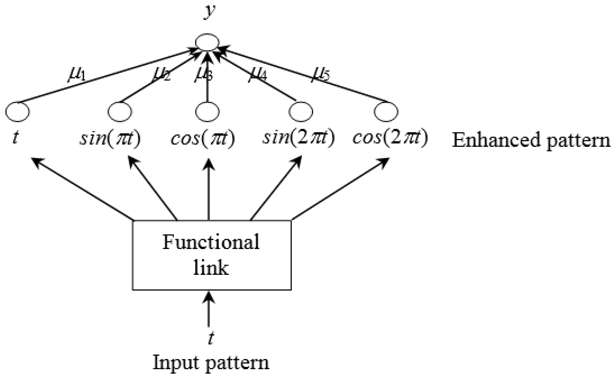
3. Residual Modification Using FLN
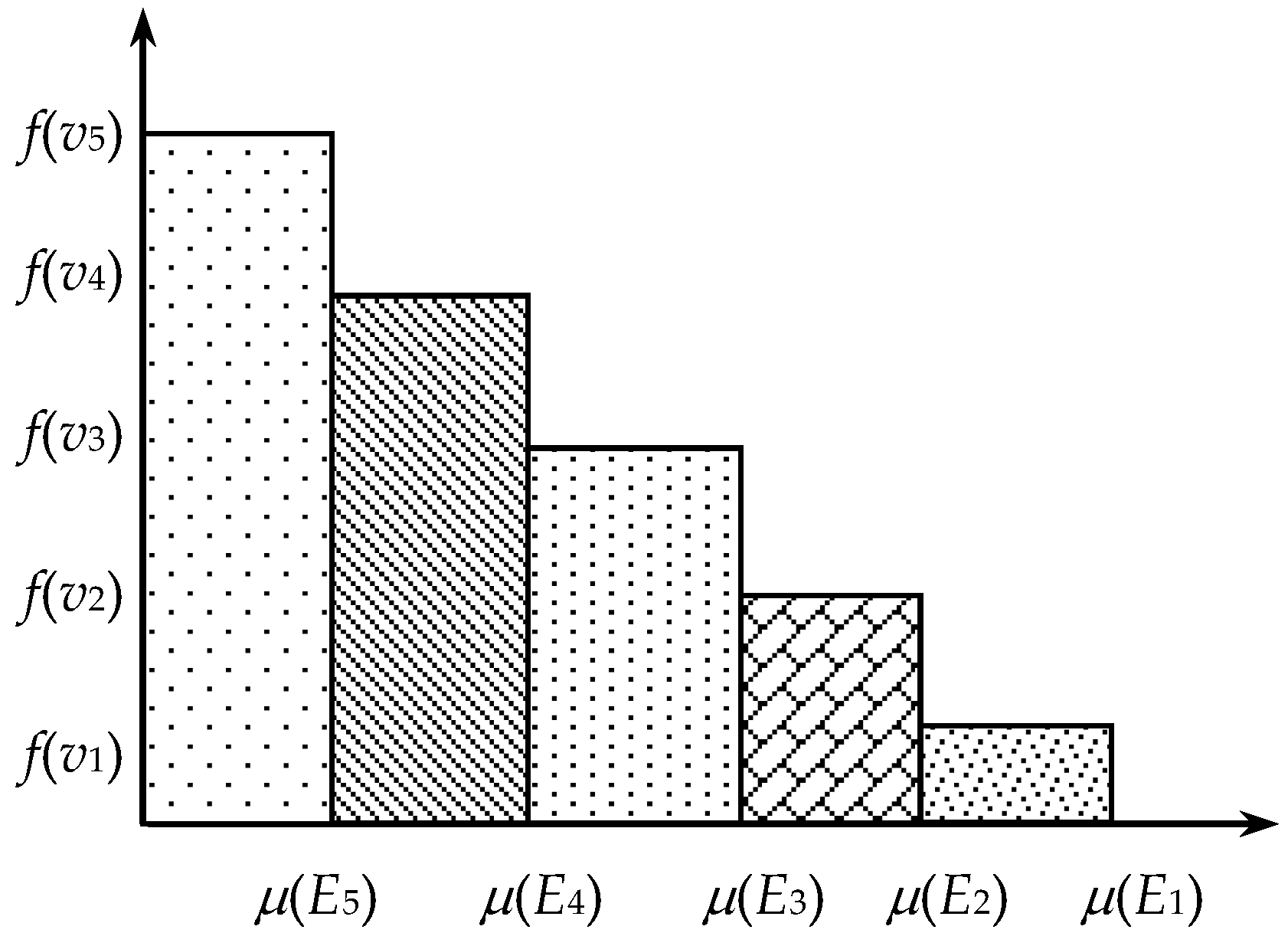
4. Nonadditive Residual Modification Model
5. Experimental Results
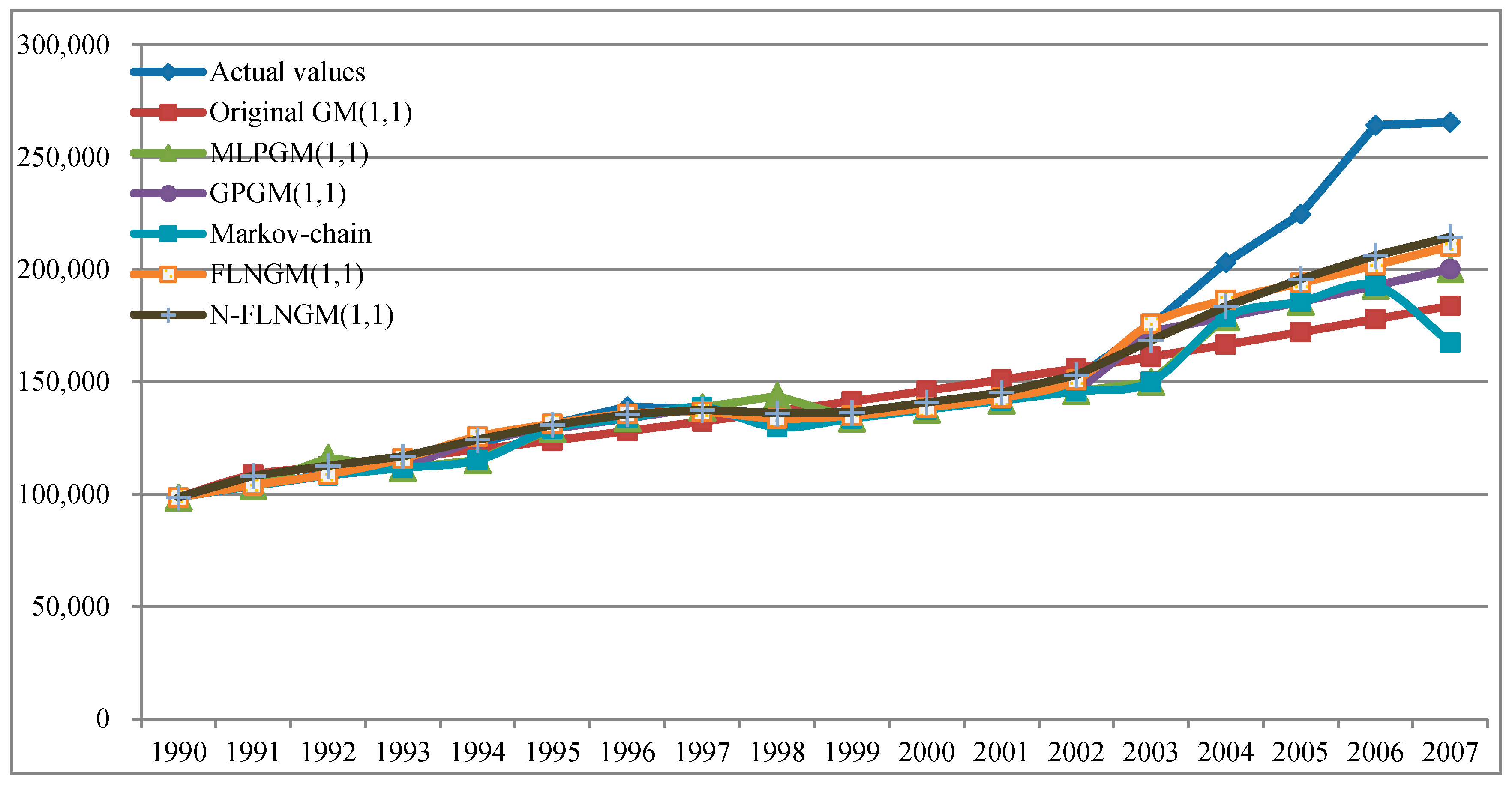
5.1. Case I
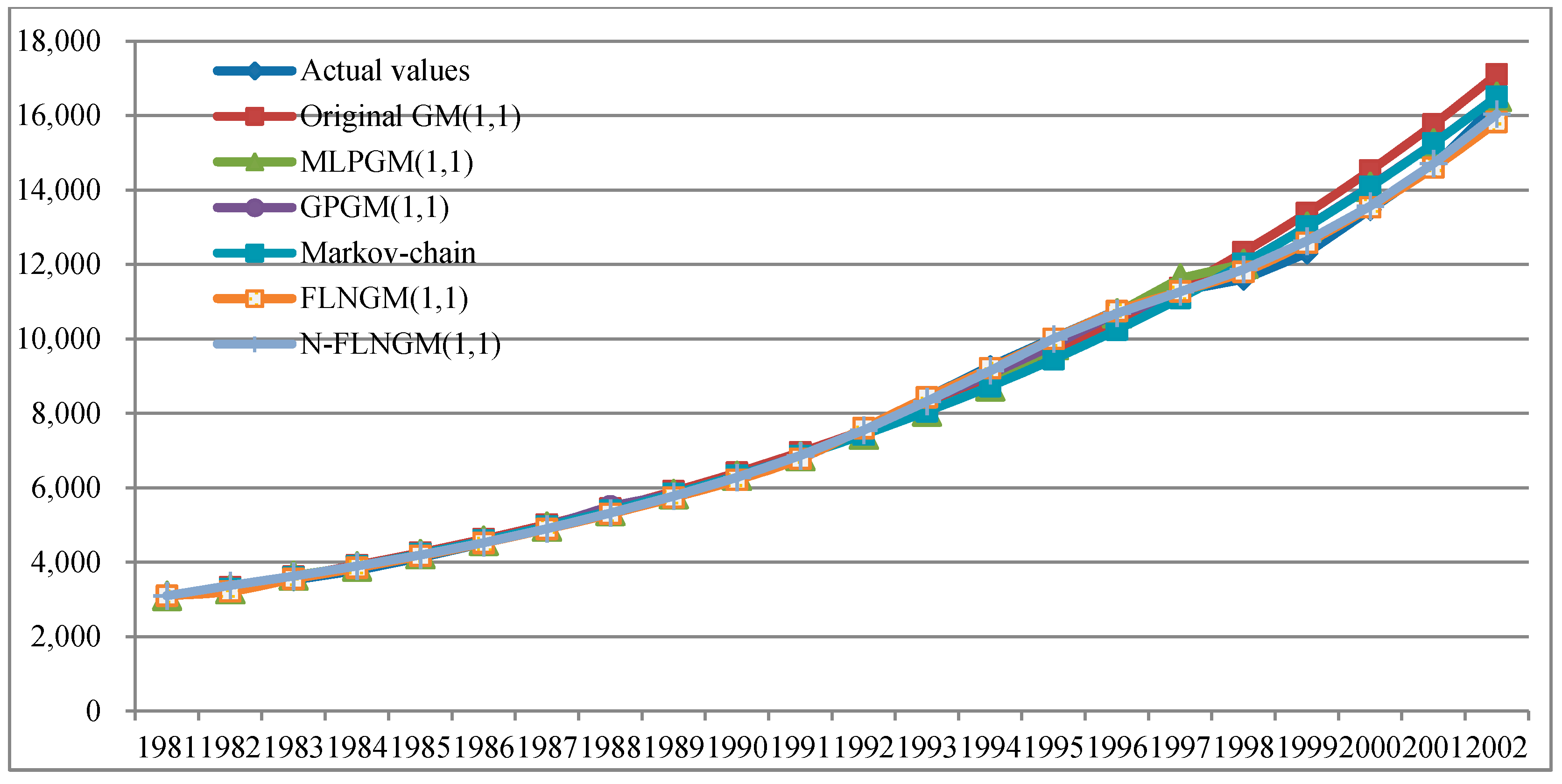
5.2. Case II
6. Discussion and Conclusions
Acknowledgments
Conflicts of Interest
References
- Taiwan Bureau of Energy. White Paper on Energy and Industrial Technology, Technical Report. Available online: https://www.moeaboe.gov.tw/ecw/populace/images/file_icon/pdf.png (accessed on 30 May 2017).
- Suganthi, L.; Samuel, A.A. Energy models for demand forecasting—A review. Renew. Sustain. Energy Rev. 2012, 16, 1223–1240. [Google Scholar] [CrossRef]
- Smith, M.; Hargroves, K.; Stasinopoulos, P.; Stephens, R.; Desha, C.; Hargroves, S. Energy Transformed: Sustainable Energy Solutions for Climate Change Mitigation; The Natural Edge Project, CSIRO, and Griffith University: Brisbane, Australia, 2007. [Google Scholar]
- Liu, Z.Y. Global Energy Internet; China Electric Power Press: Beijing, China, 2015. [Google Scholar]
- Boroojeni, K.G.; Amini, M.H.; Bahrami, S.; Iyengar, S.S.; Sarwat, A.I.; Karabasoglu, O. A novel multi-time-scale modeling for electric power demand forecasting: From short-term to medium-term horizon. Electr. Power Syst. Res. 2017, 142, 58–73. [Google Scholar] [CrossRef]
- Ediger, V.S.; Akar, S. ARIMA forecasting of primary energy demand by fuel in Turkey. Energy Policy 2007, 35, 1701–1708. [Google Scholar] [CrossRef]
- Lauret, P.; Fock, E.; Randrianarivony, R.N.; Manicom-Ramasamy, J.F. Bayesian neural network approach to short time load forecasting. Energy Convers. Manag. 2000, 49, 1156–1166. [Google Scholar] [CrossRef]
- Mohanty, S.; Patra, P.K.; Sahoo, S.S.; Mohanty, A. Forecasting of solar energy with application for a growing economy like India: Survey and implication. Renew. Sustain. Energy Rev. 2017, 78, 539–553. [Google Scholar] [CrossRef]
- Toksari, M.D. Estimating the net electricity energy generation and demand using ant colony optimization approach: Case of Turkey. Energy Policy 2009, 37, 1181–1187. [Google Scholar] [CrossRef]
- Tutun, S.; Chou, C.A.; Canıyılmaz, E. A new forecasting framework for volatile behavior in net electricity consumption: A case study in Turkey. Energy 2015, 93, 2406–2422. [Google Scholar] [CrossRef]
- Verdejo, H.; Awerkin, A.; Becker, C.; Olguin, G. Statistic linear parametric techniques for residential electric energy demand forecasting. A review and an implementation to Chile. Renew. Sustain. Energy Rev. 2017, 74, 512–521. [Google Scholar] [CrossRef]
- Xia, C.; Wang, J.; McMenemy, K.S. Medium and long term load forecasting model and virtual load forecaster based on radial basis function neural networks. Electr. Power Energy Syst. 2010, 32, 743–750. [Google Scholar] [CrossRef]
- Yang, Y.; Chen, Y.; Wang, Y.; Li, C.; Li, L. Modelling a combined method based on ANFIS and neural network improved by DE algorithm: A case study for short-term electricity demand forecasting. Appl. Soft Comput. 2016, 49, 663–675. [Google Scholar] [CrossRef]
- Wang, C.H.; Hsu, L.C. Using genetic algorithms grey theory to forecast high technology industrial output. Appl. Math. Comput. 2008, 195, 256–263. [Google Scholar] [CrossRef]
- Li, D.C.; Chang, C.J.; Chen, C.C.; Chen, W.C. Forecasting short-term electricity consumption using the adaptive grey-based approach-An Asian case. Omega 2012, 40, 767–773. [Google Scholar] [CrossRef]
- Pi, D.; Liu, J.; Qin, X. A grey prediction approach to forecasting energy demand in China, Energy Sources, Part A: Recovery. Util. Environ. Eff. 2010, 32, 1517–1528. [Google Scholar]
- Lee, Y.S.; Tong, L.I. Forecasting energy consumption using a grey model improved by incorporating genetic programming. Energy Convers. Manag. 2011, 52, 147–152. [Google Scholar] [CrossRef]
- Feng, S.J.; Ma, Y.D.; Song, Z.L.; Ying, J. Forecasting the energy consumption of China by the grey prediction model, Energy Sources, Part B: Economics. Plan. Policy 2012, 7, 376–389. [Google Scholar]
- Chen, Y.; He, K.; Zhang, C. A novel grey wave forecasting method for predicting metal prices. Resour. Policy 2016, 49, 323–331. [Google Scholar] [CrossRef]
- Li, K.; Liu, L.; Zhai, J.; Khoshgoftaar, T.M.; Li, T. The improved grey model based on particle swarm optimization algorithm for time series prediction. Eng. Appl. Artif. Intell. 2016, 55, 285–291. [Google Scholar] [CrossRef]
- Wang, Z.X.; Hao, P. An improved grey multivariable model for predicting industrial energy consumption in China. Appl. Math. Model. 2016, 40, 5745–5758. [Google Scholar] [CrossRef]
- Zeng, B.; Meng, W.; Tong, M.Y. A self-adaptive intelligence grey predictive model with alterable structure and its application. Eng. Appl. Artif. Intell. 2016, 50, 236–244. [Google Scholar] [CrossRef]
- Zhao, H.; Guo, S. An optimized grey model for annual power load forecasting. Energy 2016, 107, 272–286. [Google Scholar] [CrossRef]
- Deng, J.L. Control problems of grey systems. Syst. Control Lett. 1982, 1, 288–294. [Google Scholar]
- Liu, S.; Lin, Y. Grey Information: Theory and Practical Applications; Springer-Verlag: London, UK, 2006. [Google Scholar]
- Hsu, C.C.; Chen, C.Y. Applications of improved grey prediction model for power demand forecasting. Energy Convers. Manag. 2003, 44, 2241–2249. [Google Scholar] [CrossRef]
- Hsu, C.I.; Wen, Y.U. Improved Grey prediction models for trans-Pacific air passenger market. Transp. Plan. Technol. 1998, 22, 87–107. [Google Scholar] [CrossRef]
- Hsu, L.C. Applying the grey prediction model to the global integrated circuit industry. Technol. Forecast. Soc. Chang. 2003, 70, 563–574. [Google Scholar] [CrossRef]
- Hu, Y.C. Grey prediction with residual modification using functional-link net and its application to energy demand forecasting. Kybernetes 2017, 46, 349–363. [Google Scholar] [CrossRef]
- Hu, Y.C. Functional-link nets with genetic-algorithm-based learning for robust nonlinear interval regression analysis. Neurocomputing 2009, 72, 1808–1816. [Google Scholar] [CrossRef]
- Pao, Y.H. Adaptive Pattern Recognition and Neural Networks; Addison-Wesley: Reading, Boston, MA, USA, 1989. [Google Scholar]
- Pao, Y.H. Functional-link net computing: Theory, system architecture, and functionalities. Computer 1992, 25, 76–79. [Google Scholar] [CrossRef]
- Park, G.H.; Pao, Y.H. Unconstrained word-based approach for off-line script recognition using density-based random-vector functional-link net. Neurocomputing 2000, 31, 45–65. [Google Scholar] [CrossRef]
- Hu, Y.C. Nonadditive similarity-based single-layer perceptron for multi-criteria collaborative filtering. Neurocomputing 2014, 129, 306–314. [Google Scholar] [CrossRef]
- Hu, Y.C.; Chiu, Y.J.; Liao, Y.L.; Li, Q. A fuzzy similarity measure for collaborative filtering using nonadditive grey relational analysis. J. Grey Syst. 2015, 27, 93–103. [Google Scholar]
- Wang, Z.; Leung, K.S.; Klir, G.J. Applying fuzzy measures and nonlinear integrals in data mining. Fuzzy Sets Syst. 2005, 156, 371–380. [Google Scholar] [CrossRef]
- Wang, W.; Wang, Z.; Klir, G.J. Genetic algorithms for determining fuzzy measures from data. J. Intell. Fuzzy Syst. 1998, 6, 171–183. [Google Scholar]
- Hu, Y.C.; Tseng, F.M. Functional-link net with fuzzy integral for bankruptcy prediction. Neurocomputing 2007, 70, 2959–2968. [Google Scholar] [CrossRef]
- Murofushi, T.; Sugeno, M. An interpretation of fuzzy measure and the Choquet integral as an integral with respect to a fuzzy measure. Fuzzy Sets Syst. 1989, 29, 201–227. [Google Scholar] [CrossRef]
- Murofushi, T.; Sugeno, M. A theory of fuzzy measures: Representations, the Choquet integral, and null sets. J. Math. Anal. Appl. 1991, 159, 532–549. [Google Scholar] [CrossRef]
- Murofushi, T.; Sugeno, M. Some quantities represented by the Choquet integral. Fuzzy Sets Syst. 1993, 56, 229–235. [Google Scholar] [CrossRef]
- Goldberg, D.E. Genetic Algorithms in Search, Optimization, and Machine Learning; Addison-Wesley: Massachusetts, MA, USA, 1989. [Google Scholar]
- Montgomery, D.C. Statistical Quality Control; John Wiley & Sons: New Jersey, NJ, USA, 2005. [Google Scholar]
- Kuncheva, L.I. Fuzzy Classifier. Design; Physica-Verlag: Heidelberg, Germany, 2000. [Google Scholar]
- Sugeno, M. Fuzzy measures and fuzzy integrals: A survey. In Fuzzy Automata and Decision Processes; Gupta, M.M., Saridis, G.N., Gaines, B.R., Eds.; North Holland: New York, NY, USA, 1977; pp. 89–102. [Google Scholar]
- Sugeno, M.; Narukawa, Y.; Murofushi, Y. Choquet integral and fuzzy measures on locally compact space. Fuzzy Sets Syst. 1998, 7, 205–211. [Google Scholar] [CrossRef]
- Rooij, A.J.F.; Jain, L.C.; Johnson, R.P. Neural Network Training Using Genetic Algorithms; World Scientific: Hackensack, NJ, USA, 1996. [Google Scholar]
- Lee, S.C.; Shih, L.H. Forecasting of electricity costs based on an enhanced gray-based learning model: A case study of renewable energy in Taiwan. Technol. Forecast. Soc. Chang. 2011, 78, 1242–1253. [Google Scholar] [CrossRef]
- Makridakis, S. Accuracy measures: Theoretical and practical concerns. Int. J. Forecast. 1993, 9, 527–529. [Google Scholar] [CrossRef]
- Lewis, C. Industrial and Business Forecasting Methods; Butterworth Scientific: London, UK, 1982. [Google Scholar]
- National Bureau of Statistics of China. China Statistical Yearbook 2014; China Statistics Press: Beijing, China, 2014.
- Zhou, P.; Ang, B.W.; Poh, K.L. A trigonometric grey prediction approach to forecasting electricity demand. Energy 2006, 31, 2839–2847. [Google Scholar] [CrossRef]
- Eric, R.; Seema, S. Bankruptcy prediction by neural network. In Neural Networks in Finance and Investing: Using Artificial Intelligence to Improve Real-World Performance; Trippi, R.R., Turban, E., Eds.; McGraw-Hill: Chicago, IL, USA, 1996; pp. 243–259. [Google Scholar]
- British Petroleum. Energy Outlook, Technical Report. Available online: https://www.bp.com/content/dam/bp/pdf/energy-economics/energy-outlook-2017/bp-energy-outlook-2017.pdf (accessed on 30 May 2017).
- Yager, R.R. Elements selection from a fuzzy subset using the fuzzy integral, IEEE Transactions on Systems. Man Cybern. 1993, 23, 467–477. [Google Scholar] [CrossRef]
- Hu, Y.C.; Tzeng, G.H.; Hsu, Y.T.; Chen, R.S. Using learning algorithm to find the developing coefficient and control variable of GM(1,1) model. J. Chin. Grey Syst. Assoc. 2001, 4, 17–26. [Google Scholar]


| Year | Actual | GM(1,1) | MLPGM(1,1) | GPGM(1,1) | Markov-Chain | FLNGM(1,1) | N-FLNGM(1,1) | ||||||
|---|---|---|---|---|---|---|---|---|---|---|---|---|---|
| Predicted | APE | Predicted | APE | Predicted | APE | Predicted | APE | Predicted | APE | Predicted | APE | ||
| 1990 | 98,703 | 98,703 | 0 | 98,703 | 0 | 98,703 | 0 | 98,703 | 0 | 98,703 | 0 | 98,703 | 0 |
| 1991 | 103,783 | 108,706.1 | 4.74 | 103,783 | 0 | 103,783 | 0 | 103,783 | 0 | 104,116.2 | 0.32 | 108,332.5 | 4.38 |
| 1992 | 109,170 | 112,335.5 | 2.9 | 116,225.8 | 6.46 | 108,445.2 | 0.66 | 108,445.2 | 0.66 | 108,913.6 | 0.23 | 112,708.3 | 3.24 |
| 1993 | 115,993 | 116,086.1 | 0.08 | 111,804.1 | 3.61 | 111,804.1 | 3.61 | 111,804.1 | 3.61 | 115,973.2 | 0.02 | 116,938.2 | 0.82 |
| 1994 | 122,737 | 119,962 | 2.26 | 115,248.8 | 6.10 | 124,675.1 | 1.58 | 115,248.8 | 6.10 | 125,629.8 | 2.36 | 124,309.9 | 1.28 |
| 1995 | 131,176 | 123,967.2 | 5.50 | 129,154.8 | 1.54 | 129,154.8 | 1.54 | 129,154.8 | 1.54 | 131,380.7 | 0.16 | 130,842 | 0.25 |
| 1996 | 138,948 | 128,106.2 | 7.80 | 133,816.1 | 3.69 | 133,816.1 | 3.69 | 133,816.1 | 3.69 | 135,703.7 | 2.33 | 135,615.4 | 2.40 |
| 1997 | 137,798 | 132,383.3 | 3.93 | 138,668.2 | 0.63 | 138,668.2 | 0.63 | 138,668.2 | 0.63 | 136,710.1 | 0.79 | 137,554.2 | 0.18 |
| 1998 | 132,214 | 136,803.3 | 3.47 | 143,721 | 8.7 | 129,885.5 | 1.76 | 129,885.5 | 1.76 | 133,735.8 | 1.15 | 136,059.7 | 2.92 |
| 1999 | 133,831 | 141,370.8 | 5.63 | 133,756.5 | 0.06 | 133,756.5 | 0.06 | 133,756.5 | 0.06 | 135,005.6 | 0.88 | 136,387.9 | 1.92 |
| 2000 | 138,553 | 146,090.8 | 5.44 | 137,709.8 | 0.61 | 137,709.8 | 0.61 | 137,709.8 | 0.61 | 138,603.2 | 0.04 | 140,826.2 | 1.65 |
| 2001 | 143,199 | 150,968.4 | 5.43 | 141,743.6 | 1.02 | 141,743.6 | 1.02 | 141,743.6 | 1.02 | 142,946.8 | 0.18 | 145,273.3 | 1.45 |
| 2002 | 151,797 | 156,008.9 | 2.77 | 145,855.2 | 3.91 | 145,855.2 | 3.91 | 145,855.2 | 3.91 | 150,954.8 | 0.55 | 153,016.6 | 0.81 |
| 2003 | 174,990 | 161,217.6 | 7.87 | 150,041.6 | 14.26 | 172,393.5 | 1.48 | 150,041.6 | 14.26 | 175,848.7 | 0.49 | 168,529.3 | 3.69 |
| MAPE | 4.13 | 3.61 | 2.59 | 2.70 | 0.68 | 1.78 | |||||||
| 2004 | 203,227 | 166,600.2 | 18.02 | 178,901.5 | 11.97 | 178,901.5 | 11.97 | 178,901.5 | 11.97 | 186,450.1 | 8.26 | 183,696.6 | 9.61 |
| 2005 | 224,682 | 172,162.6 | 23.37 | 185,702.4 | 17.35 | 185,702.4 | 17.35 | 185,702.4 | 17.35 | 194,058.0 | 13.63 | 195,771.8 | 12.87 |
| 2006 | 264,270 | 177,910.7 | 32.68 | 192,813.8 | 27.04 | 192,813.8 | 27.04 | 192,813.8 | 27.04 | 202,011.1 | 23.56 | 206,254.6 | 21.95 |
| 2007 | 265,583 | 183,850.7 | 30.77 | 200,254.3 | 24.60 | 200,254.3 | 24.60 | 167,447.1 | 36.95 | 210,377.6 | 20.79 | 214,426.9 | 19.26 |
| MAPE | 26.21 | 20.23 | 20.23 | 23.22 | 16.56 | 15.92 | |||||||
| Year | Actual | GM(1,1) | MLPGM(1,1) | GPGM(1,1) | Markov-chain | FLNGM(1,1) | N-FLNGM(1,1) | ||||||
|---|---|---|---|---|---|---|---|---|---|---|---|---|---|
| Predicted | APE | Predicted | APE | Predicted | APE | Predicted | APE | Predicted | APE | Predicted | APE | ||
| 1981 | 3096 | 3096 | 0 | 3096 | 0 | 3096 | 0 | 3096 | 0 | 3096 | 0 | 3096 | 0 |
| 1982 | 3280 | 3327.7 | 1.45 | 3280 | 0 | 3280 | 0 | 3280 | 0 | 3214.3 | 2.00 | 3374.4 | 2.88 |
| 1983 | 3519 | 3611.5 | 2.63 | 3638.0 | 3.38 | 3585.0 | 1.88 | 3585.0 | 1.88 | 3548.5 | 0.84 | 3625.0 | 3.01 |
| 1984 | 3778 | 3919.5 | 3.75 | 3888.3 | 2.92 | 3888.3 | 2.92 | 3888.3 | 2.92 | 3845.3 | 1.78 | 3893.6 | 3.06 |
| 1985 | 4118 | 4253.9 | 3.30 | 4217.1 | 2.41 | 4217.1 | 2.41 | 4217.1 | 2.41 | 4166.4 | 1.18 | 4189.4 | 1.73 |
| 1986 | 4507 | 4616.7 | 2.43 | 4573.3 | 1.47 | 4573.3 | 1.47 | 4573.3 | 1.47 | 4513.6 | 0.15 | 4523.1 | 0.36 |
| 1987 | 4985 | 5010.5 | 0.51 | 4959.4 | 0.51 | 4959.4 | 0.51 | 4959.4 | 0.51 | 4889.0 | 1.93 | 4897.4 | 1.76 |
| 1988 | 5467 | 5437.9 | 0.53 | 5377.6 | 1.63 | 5498.2 | 0.57 | 5377.6 | 1.63 | 5294.7 | 3.15 | 5320.3 | 2.68 |
| 1989 | 5865 | 5901.7 | 0.63 | 5830.7 | 0.59 | 5830.7 | 0.59 | 5830.7 | 0.59 | 5733.0 | 2.25 | 5775.0 | 1.53 |
| 1990 | 6230 | 6405.1 | 2.81 | 6321.4 | 1.47 | 6321.4 | 1.47 | 6321.4 | 1.47 | 6209.5 | 0.33 | 6276.4 | 0.74 |
| 1991 | 6775 | 6951.4 | 2.60 | 6852.8 | 1.15 | 6852.8 | 1.15 | 6852.8 | 1.15 | 6777.9 | 0.04 | 6859.8 | 1.25 |
| 1992 | 7542 | 7544.3 | 0.03 | 7428.1 | 1.51 | 7428.1 | 1.51 | 7428.1 | 1.51 | 7596.7 | 0.72 | 7545.1 | 0.04 |
| 1993 | 8426.5 | 8187.8 | 2.83 | 8050.8 | 4.46 | 8324.8 | 1.21 | 8050.8 | 4.46 | 8425.2 | 0.02 | 8319.0 | 1.28 |
| 1994 | 9260.4 | 8886.2 | 4.04 | 8724.8 | 5.78 | 9047.6 | 2.30 | 8724.8 | 5.78 | 9207.4 | 0.57 | 9144.2 | 1.25 |
| 1995 | 10,023.4 | 9644.1 | 3.78 | 9834.3 | 1.89 | 9834.3 | 1.89 | 9453.9 | 5.68 | 10,000.4 | 0.23 | 10,000.1 | 0.23 |
| 1996 | 10,764.3 | 10,466.7 | 2.76 | 10,690.9 | 0.68 | 10,690.9 | 0.68 | 10,242.5 | 4.85 | 10,742.7 | 0.20 | 10,685.5 | 0.73 |
| 1997 | 11,284.4 | 11,359.5 | 0.67 | 11,623.7 | 3.01 | 11,095.3 | 1.68 | 11,095.3 | 1.68 | 11,273.8 | 0.09 | 11,264.8 | 0.17 |
| 1998 | 11,598.4 | 12,328.4 | 6.29 | 12,017.1 | 3.61 | 12,017.1 | 3.61 | 12,017.1 | 3.61 | 11,796.7 | 1.71 | 11,866.7 | 2.31 |
| MAPE | 2.28 | 2.03 | 1.44 | 2.31 | 0.10 | 0.13 | |||||||
| 1999 | 12,305.2 | 13,379.9 | 8.73 | 13,013 | 5.75 | 13,013.0 | 5.75 | 13,013.0 | 5.75 | 12,581.9 | 2.25 | 12,627.3 | 2.62 |
| 2000 | 13,471.4 | 14,521.2 | 7.79 | 14,088.8 | 4.58 | 14,088.8 | 4.58 | 14,088.8 | 4.58 | 13,535.1 | 0.47 | 13,565.9 | 0.70 |
| 2001 | 14,633.5 | 15,759.8 | 7.70 | 15,250.3 | 4.21 | 15,250.3 | 4.21 | 15,250.3 | 4.21 | 14,598.4 | 0.24 | 14,710.7 | 0.53 |
| 2002 | 16,331.5 | 17,104 | 4.73 | 16,503.6 | 1.05 | 16,503.5 | 1.05 | 16,503.5 | 1.05 | 15,821.4 | 3.12 | 16,040.2 | 1.78 |
| MAPE | 7.24 | 3.90 | 3.90 | 3.90 | 1.52 | 1.41 | |||||||
| Year | Actual | MLP | N-FLNGM(1,1) | ||
|---|---|---|---|---|---|
| Predicted | APE | Predicted | APE | ||
| 1990 | 98,703 | 93,012.6 | 5.77 | 987,03 | 0 |
| 1991 | 103,783 | 107,674.6 | 3.75 | 108,332.5 | 4.38 |
| 1992 | 109,170 | 116,921.0 | 7.10 | 112,708.3 | 3.24 |
| 1993 | 115,993 | 122,130.4 | 5.29 | 116,938.2 | 0.82 |
| 1994 | 122,737 | 125,034.6 | 1.87 | 124,309.9 | 1.28 |
| 1995 | 131,176 | 126,861.3 | 3.29 | 130,842 | 0.25 |
| 1996 | 138,948 | 128,373.0 | 7.61 | 135,615.4 | 2.40 |
| 1997 | 137,798 | 130,080.1 | 5.60 | 137,554.2 | 0.18 |
| 1998 | 132,214 | 132,407.0 | 0.15 | 136,059.7 | 2.92 |
| 1999 | 133,831 | 135,788.9 | 1.46 | 136,387.9 | 1.92 |
| 2000 | 138,553 | 140,696.7 | 1.55 | 140,826.2 | 1.65 |
| 2001 | 143,199 | 147,565.7 | 3.05 | 145,273.3 | 1.45 |
| 2002 | 151,797 | 156,595.8 | 3.16 | 153,016.6 | 0.81 |
| 2003 | 174,990 | 167,469.6 | 4.30 | 168,529.3 | 3.69 |
| MAPE | 3.85 | 1.78 | |||
| 2004 | 203,227 | 179,212.1 | 11.82 | 183,696.6 | 9.61 |
| 2005 | 224,682 | 190,465.4 | 15.23 | 195,771.8 | 12.87 |
| 2006 | 264,270 | 200,083.0 | 24.29 | 206,254.6 | 21.95 |
| 2007 | 265,583 | 207,546.2 | 21.85 | 214,426.9 | 19.26 |
| MAPE | 18.30 | 15.92 | |||
| Year | Actual | MLP | N-FLNGM(1,1) | ||
|---|---|---|---|---|---|
| Predicted | APE | Predicted | APE | ||
| 1981 | 3096 | 2947.5 | 4.80 | 3096 | 0 |
| 1982 | 3280 | 3255.4 | 0.75 | 3374.4 | 2.88 |
| 1983 | 3519 | 3573.7 | 1.55 | 3625.0 | 3.01 |
| 1984 | 3778 | 3900.4 | 3.24 | 3893.6 | 3.06 |
| 1985 | 4118 | 4234.9 | 2.84 | 4189.4 | 1.73 |
| 1986 | 4507 | 4579.0 | 1.60 | 4523.1 | 0.36 |
| 1987 | 4985 | 4938.1 | 0.94 | 4897.4 | 1.76 |
| 1988 | 5467 | 5323.1 | 2.63 | 5320.3 | 2.68 |
| 1989 | 5865 | 5752.7 | 1.91 | 5775.0 | 1.53 |
| 1990 | 6230 | 6253.5 | 0.38 | 6276.4 | 0.74 |
| 1991 | 6775 | 6855.1 | 1.18 | 6859.8 | 1.25 |
| 1992 | 7542 | 7575.5 | 0.44 | 7545.1 | 0.04 |
| 1993 | 8426.5 | 8396.8 | 0.35 | 8319.0 | 1.28 |
| 1994 | 9260.4 | 9252.6 | 0.08 | 9144.2 | 1.25 |
| 1995 | 10,023.4 | 10,051.4 | 0.28 | 10,000.1 | 0.23 |
| 1996 | 10,764.3 | 10,724.4 | 0.37 | 10,685.5 | 0.73 |
| 1997 | 11,284.4 | 11,250.6 | 0.30 | 11,264.8 | 0.17 |
| 1998 | 11,598.4 | 11,646.4 | 0.41 | 11,866.7 | 2.31 |
| MAPE | 1.34 | 0.13 | |||
| 1999 | 12,305.2 | 11,942.1 | 2.95 | 12,627.3 | 2.62 |
| 2000 | 13,471.4 | 12,166.3 | 9.69 | 13,565.9 | 0.70 |
| 2001 | 14,633.5 | 12,341.1 | 15.67 | 14,710.7 | 0.53 |
| 2002 | 16,331.5 | 12,481.5 | 23.57 | 16,040.2 | 1.78 |
| MAPE | 12.97 | 1.41 | |||
© 2017 by the author. Licensee MDPI, Basel, Switzerland. This article is an open access article distributed under the terms and conditions of the Creative Commons Attribution (CC BY) license (http://creativecommons.org/licenses/by/4.0/).
Share and Cite
Hu, Y.-C. Nonadditive Grey Prediction Using Functional-Link Net for Energy Demand Forecasting. Sustainability 2017, 9, 1166. https://doi.org/10.3390/su9071166
Hu Y-C. Nonadditive Grey Prediction Using Functional-Link Net for Energy Demand Forecasting. Sustainability. 2017; 9(7):1166. https://doi.org/10.3390/su9071166
Chicago/Turabian StyleHu, Yi-Chung. 2017. "Nonadditive Grey Prediction Using Functional-Link Net for Energy Demand Forecasting" Sustainability 9, no. 7: 1166. https://doi.org/10.3390/su9071166
APA StyleHu, Y.-C. (2017). Nonadditive Grey Prediction Using Functional-Link Net for Energy Demand Forecasting. Sustainability, 9(7), 1166. https://doi.org/10.3390/su9071166