Measuring Sustainable Competitiveness in Contemporary Economies—Insights from European Economy

Abstract

The recent transformation of the national economies has raised numerous theoretical and practical aspects in measuring economic growth, welfare, environmental performance, and competitiveness, representing a challenging research topic within the context of economic paradigm transformation. Despite its importance, a fully operational model to be used in any context has not yet been designed. The main aim of this paper is to evaluate and analyze the macroeconomic dimension of the three determinants of sustainable competitiveness: the economic environment, the social environment, and the natural environment, at both the European and Romanian levels. This paper used the Hierarchical Clustering methodology, aiming at evaluating the global competitiveness in terms of a sustainable development model, using four indices: Human Development Index, Environmental Performance Index, Global Competitiveness Index, and GDP per capita. The clusters were designed on the basis of the role of the indices in assessment of the sustainable performances of the countries and also of the possible convergences between them. The results could sustain the conclusion that these indices are not able to offer an exhaustive image of the sustainable performances assessment. A new complex indicator could be considered in order to design a convergence model for the EU member states.

1. Introduction

Sustainable development is an essential factor in creating new added value and innovation, while at the same time being able to contribute decisively to the economic development of individuals and society as a whole. In a free market and a well-functioning economy [1,2], sustainable development could provide equilibrium between economic prosperity, social cohesion, and rational usage of natural resources in order to assure production dematerialization by decoupling economic growth from intensive development. Sustainable development and green economy are conditioned by the existence of two main elements: the first is the promotion of the rational use of available economic resources and the other is generated by growing competition from emerging countries in obtaining economic resources that are increasingly fewer and becoming more expensive in terms of availability.

Sustainable growth has become a discussion topic in the literature [3,4], especially since the 1980s [4], when researchers became interested in the links between sustainability and the economy and how these links may be inter-related. Measuring sustainable development is a subject [5,6] that elicits various approaches both in terms of conceptual transformations, measuring instruments, and achievement. The main benefits of a sustainable economy [7] are the design of a new economic paradigm by promoting global economic competitiveness, the intelligent use of resources, extending product life, and new job opportunities. In this context, the multifaceted concept of sustainable competitiveness must be effectively put in relation with national competitiveness [8]. In a global and multifunctional economy, measuring the sustainable competitiveness represents a challenge for scholars and practitioners in order to assess sustainable development in all its dimensions—economic, social, and human wellbeing.

Identification of those policy tools enhancing the sustainable competitiveness of the national economy is a difficult problem. In many cases, they come to contradict long-term growth objectives. The development of a new and resilient economy through sustainable investments and financial allotments increase the possibility of a new and more competitive economy.

Sustainable development policies aim at the establishment of an economic, social, and environmental evaluation system of the impact of economic activity on the environment. To analyze these issues, several categories of indicators are used in the literature, including: Environmental Sustainability Index (ESI), Environmental Performance Index (EPI), Climate Change Performance Index (CCPI), Human Development Index (HDI), Index of Sustainable Economic Welfare (ISEW) and Global Competitiveness Index (GCI). Costanza et al. [9] emphasized the need to replace an excessive use of Gross Domestic Product (GDP) as an indicator of national performance, not only with an alternative indicator of welfare, but also with a complex indicator that considers society as a dynamic system that is in permanent exchange with the natural environment.

Following hierarchies based on these indicators, differences are noted. Our paper shows the need to develop a new comprehensive indicator that exhaustively measures the level of sustainable competitiveness. Our analysis aims at evaluating the global competitiveness in terms of a sustainable development model, taking into account all three levels: economic, social, and environmental. The economic dimension is measured by GDP per capita, and the environmental dimension is measured by EPI. The other two dimensions are measured using the HDI. We introduced the HDI in the analysis because we considered this indicator to be more complex than GDP per capita. HDI is constructed by considering the social dimension—by the health field and the education field—in addition to the economic dimension. The national competitiveness is measured by GCI.

Until the end of the 90s decade, economists had considered that the GDP was one of the most important indicators used to measure economic performance. The political decision factors considered that GDP was an index capable of measuring a nation’s degree of development and welfare. At the end of the 90s decade, Nordhaus et al. [10,11,12,13] did not consider GDP an appropriate index for environmental protection as an important element for sustainable development. Economists such as [14,15,16] were interested in the links between sustainability and the economy and how these links can be interdependent.

Ecologists such as [17,18] have been interested in the environmental medium and the ecological footprint to be able to model and develop macroeconomic sustainability measures. The measures developed can be classified into these categories:

• Measures directed to economic medium;
• Measures directed to ecological medium;
• Measures directed to social medium.

The measures directed to economic medium are those based on the conventional economic background. This category may integrate Green NDP/NNP [19], income distribution adjusted GDP [20], Genuine Savings [19,21], Generational Environmental Debt [22,23], and the Index of Sustainable Economic Welfare [13].

The measures directed to the ecologic medium are those based on the Ecological Footprint [17] and Environmental Space [18].

The measures directed to the social medium are those based on society. These measures describe the social status, the distribution of income in society, the unemployment rate, the literacy rate, and the educational level from the urban and rural medium. Social performance indicators can influence the organization’s intangible assets, such as human capital and reputation [24]. HDI is the most known social development index [25].

In the United Nations Development Programme (UNDP), a “Human Development Report” was published in 1990. The main contribution of this report is the calculation of the Human Development Index. This index was suggested by [26]. In determining the HDI, four types of indicators for the three fields were used. These indicators and these fields are essential for evaluating human development and quality of life. The HDI measures the degree to which a country successfully develops its human capital. HDI is considered useful because it has a greater coverage than GDP, taking into account other socio-economic indicators in addition to it, while GDP per capita measures only material prosperity. The concept of human development highlights this indicator, which reveals the structure and direction of progress (or regress) of human capital in the sustainable growth frame of an economy.

HDI is designed by aggregating three categories of indicators, namely:

• For the economic field—the standard of living—Gross Domestic Product (GDP) per capita purchasing power parity calculated is used as a measure of standard of living to express the welfare of a sustainable economy (economic standard);
• For the health sector—longevity (average life expectancy)—is measured by life expectancy at birth, which is directly influenced by the level of development of the country;
• For the field of education—two indicators are used, namely: level of adult literacy (it has a weight of two-thirds) and a combined gross enrolment ratio (CGER), incorporating all three levels of education (which has a weight of one-third).

Thus, the HDI reflects the achievements in three key areas: a long and healthy life, a decent education, and a decent living standard. All these aspects are directly correlated with factors contributing to the quality of life; i.e., material welfare, people quality, and quality of the economic and social system.

Environmental performance is measured with the Environmental Performance Index (EPI). This index was drawn up by a group of environmental experts at Yale University and Columbia University. According to them, this index ranks countries according to their performance in the domain of environmental issues which regard two areas of general policy: protection of human health and protection of ecosystems. The two pillars of the EPI structure are environmental health and the vitality of the ecosystem. Environmental health assesses the degree of human health protection against the negative effects on the environment. Three categories of issues are measured for this goal: Health Impacts, Air Quality, and Water and Sanitation. Ecosystem vitality assesses ecosystem protection and resource management. Six categories of issues are assessed for this purpose: Water Resources, Agriculture, Forests, Fisheries, Biodiversity and Habitat, and Climate and Energy. In order to assess these issues, 20 national indicators reflecting environmental data are calculated and aggregated. The data sets for the calculation of these indicators are provided by national government reports, the World Bank, the UN Development Program, the United Nations, and the World Resources Institute [27].

In this respect, Lober [28] considers that the connection between the reliable results of the organizations and environmental protection is based on elements such as maintaining the quality of water, air, and soil. For his part, Epstein [29] has been interested in components of environmental performance such as:

• Minimization and control of pollutants;
• Waste reduction;
• Conserving resources and energy conservation.

This index has been used since 2006. Before this, the Environmental Sustainability Index (ESI) has been used. ESI is a composite index published during 1999–2005 built on 21 performance indicators that reflect national environmental data, grouped in five categories of policies aiming at sustainability [30]:

• Environmental system condition;
• Reduction of environmental stress;
• Reduction of human vulnerability;
• Societal and institutional capacities to respond to environmental challenges;
• Global environmental responsibility [31].

The Environmental Performance Index was designed with the purpose of transnational use. It was found that EPI is a more complex quantitative indicator which is results-oriented and can be easily used by policy makers [32]. That’s why it was decided to use it in official World Economic reports. In addition, the authors considered to draw attention to the fact that there is a shortage of information on many substances and their effects on the environment and human health at an international level. The importance of making environmental data collection uniform at an international level is emphasized. Thus, The EPI-Team explicitly considers that the activity regarding the EPI should be seen as a work-in-progress [31].

The Global Competitiveness Index (GCI) measures national competitiveness, requiring annual data collection from many countries. Its purpose is to assess the competitiveness of the country to achieve productivity, economic growth, and sustained economic prosperity [33]. It is based on a set of three key factors considered essential for a country’s level of productivity and efficiency [20]. These are the basic factors (public institutions, infrastructure, macroeconomic development, health, and primary education), efficiency factors (higher development and training in human resources, market efficiency, responsiveness to new technologies, labor market efficiency, financial market development), and innovation factors (market size, business sophistication, and innovation).

The GCI can be distinguished by the inclusion of many indicators as determinant variables. They are pragmatically selected based on theoretical aspects explaining prosperity. The factors are grouped hierarchically into categories depending on how they affect competitiveness. Regarding the issues to be considered when selecting indicators, two aspects are to be mentioned—namely, taxation policies and regulatory policies in the labor market because they have no simple linear relationship with prosperity. Thus, especially in developed countries, tax rates appear to be higher in countries with strong institutions, whose investments in social services are more rational However, the case of the less-developed countries must be mentioned, because these also have important level of taxation, but their spending in the public system is less efficient (unfortunately, this seems to be the situation in Romania). Thus, the econometric effect on competitiveness is harder to determine. The GCI requires the annual gathering of data from many countries, aiming to offer a framework to inform overall policy while establishing priorities at the specific policy level [34]. Thus, the GCI model aims to determine a general classification of countries according to competitiveness, in order to build an overall predictor of productivity.

The economic performance (measured with GDP, HDI, and GCI) contributes to maintaining and even to developing profitability in the short, medium, and long-term at the micro- and macroeconomic levels. Social performance (measured with HDI and GCI) contributes to obtaining: welfare for all members of society; equity and social justice; social inclusion, cohesion, and solidarity; and an adequate level of health and education for the population. These last two principles could be related to eco-welfare. Environmental performance (measured with EPI and GCI) contributes to maintaining a stable base of natural resources and avoiding as much as possible excessive exploitation of non-renewable resources. These variables have been analyzed since 2008 because we assumed that the economic recession could generate some effects. GCI’s evolution can be explained by the fact that it measures how efficiently a country uses available resources and the capacity of the state to ensure a high standard of living for its citizens. Different authors have identified different types of relationships between different indicators [24].

The focus of our research is on the possibility of grouping countries in terms of the assessment of the sustainable competitiveness of the European countries and in particular to a transitional country such as Romania. As we have shown above, a comprehensive indicator for assessing a country’s sustainable competitiveness has not yet been constructed. This situation is explained by the diversity of the issues to be considered and the inhomogeneity of data describing those issues. The question is whether there is a suitable development model for Romania which could help in reducing gaps between Romania and EU-28 average in terms of competitiveness. The approach of this subject has started from the following question: do those countries showing high values of GDP or GCI also have high levels of EPI or HDI? Our objective is to look for the possible existence of a convergence of the countries belonging to the same group.

This paper aimed to consider the macroeconomic vision of the three determinants of sustainable development: the economic environment, the social environment, and the natural environment, looking for a relevant image of the countries’ grouping in these terms. In this respect, the paper was structured in analyzing the following three major aspects:

-

The existence of some groups of countries which are significant in terms of the analyzed indicator;

-

The existence of some overlaps of the identified clusters;

-

The analysis of the evolutions of these indexes in the case of Romania.

2. Materials and Methods

2.1. Data

In order to achieve the research goals, the authors have chosen to group the EU-28 Members States, except Malta, but including Switzerland, Norway and Iceland. Malta was excluded because of the lack of data for EPI in 2008. Switzerland, Norway, and Iceland were included because of their similitudes with the rich states of the EU having a prominent level of welfare.

The period 2008–2014 represents the full-time coverage of the used variables—namely, HDI, EPI, GCI, and GDP (expressed as Main GDP aggregates per capita considered according to Eurostat as the newest internationally compatible EU accounting framework for a systematic and detailed description of an economy (http://ec.europa.eu/eurostat/cache/metadata/en/namq_10_esms.htm)) [33,35,36,37,38,39,40].

HDI values were retrieved from Human Development Reports published by the United Nations Development Programme [33]. EPI values were retrieved from the EPI Reports elaborated at Yale University [35]. These reports are available annually from 2006, except for 2009 and 2011. For this reason, the data set used for the analysis is annual over two-year increments. Data for GCI were obtained from the Global Competitiveness Reports prepared by the World Economic Forum. These reports are also annual. Eurostat was the source of data for GDP [40]. Nominal GDP was used (unit of measure: current prices, Euro per capita). Given that the aim was not to measure output, we considered the nominal GDP acceptable.

Analyzing the figures in the descriptive statistics table, we can notice the following:

Regarding HDI, the average value continuously increased during the analyzed period. The gap in HDI values reduced in 2010. Then, after a slight increase in 2012, it declined again significantly. This could represent the effect of the concerted efforts made by the EU members in order to diminish the gaps in human development.

The same thing cannot be said about GDP. Thus, the evolution of the average values looks similar, but the spread has steadily increased. This suggests that the economic performances of the EU members still remain very different, while the gaps continue to increase.

Regarding EPI, it may be noticed that its average value of this index continuously decreased until 2012, and an increase can be observed in 2014. The spread had a fluctuating evolution. After a fairly significant increase in 2010, a fall followed in 2012, then, again, an increase in 2014. However, it should be taken into account that the methodology for calculating this index has changed since 2014.

Regarding GCI, the average of this index followed the same trend as in the case of HDI and GDP. Thus, a decrease occurred in 2010. This decrease can be linked to the effects of the economic crisis. However, it was followed by a continuous increase. GCI’s range grew steadily until 2012, after which it declined in 2014. This suggests that EU policy efforts to reduce the competitiveness gap between the Member States began to bear fruit after 2012.

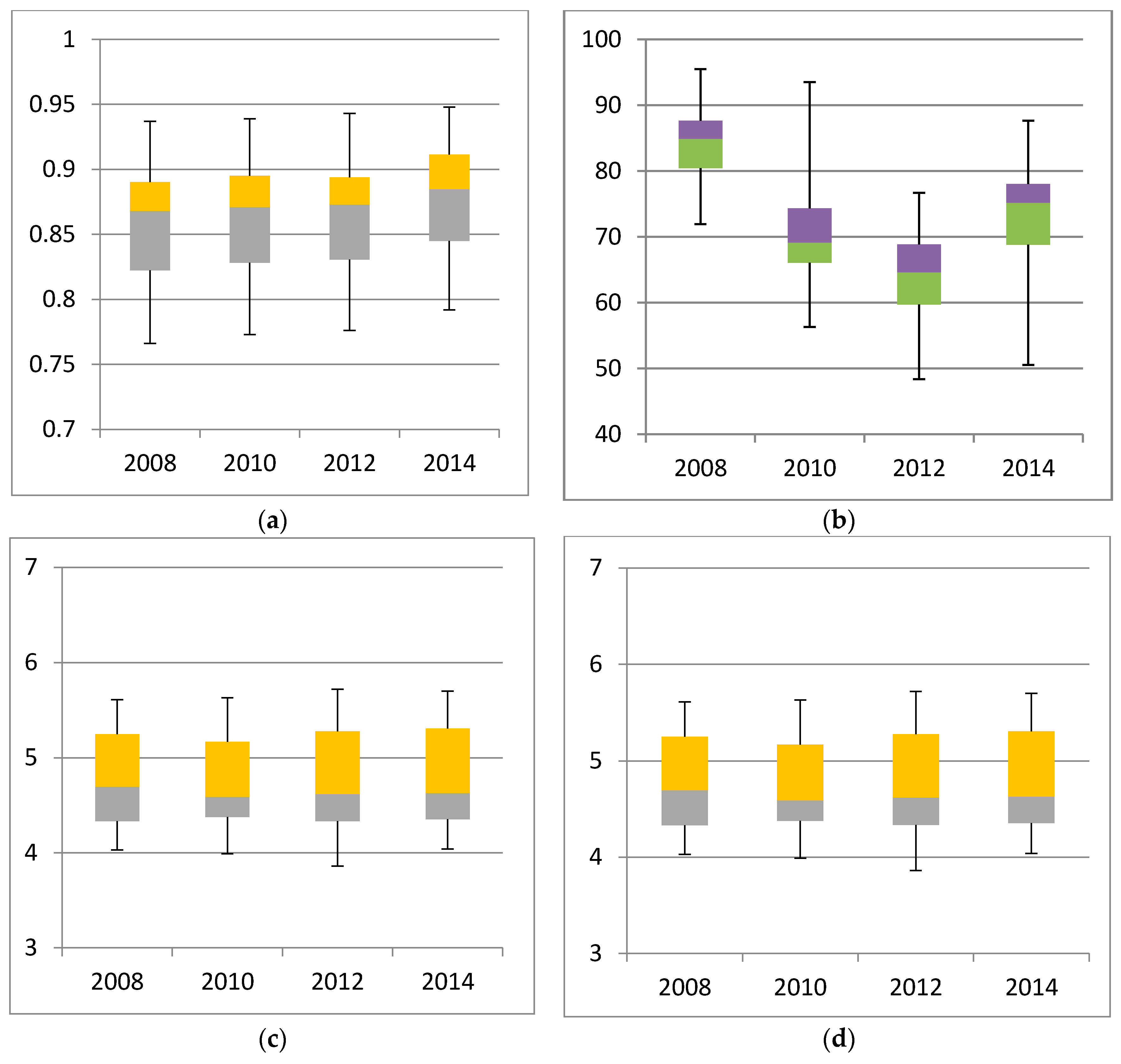
To further illustrate the behavior of these indicators, the whisker plots for data set were built (Figure 1).

The following comments can be made based on whisker plots (Figure 1):

Regarding HDI, it may be noticed that the highest degree of values dispersion was in 2008, just after the last wave of accession to the EU. Later, it began to diminish. Additionally, it is to be noticed that there is a larger range of values for the first half of the data, with the values from the second half being close together. This issue was more emphasized at the beginning of the study period.

Things are different in terms of GDP values. Thus, the plot indicates that the highest 25% of the data is spread over a larger range than the lowest 25%. Therefore, the hierarchy of the poor countries is closer than that of the rich ones.

In the case of EPI, a reversal of the situation occurred in 2010 compared to 2008. Thus, the spread of values has significantly increased, and the hierarchy has become stronger at the beginning of the ranking.

2.2. Methodology

To achieve the assumed goal, the authors used cluster analysis, which leads to the grouping of a set of similar group observations to allow tagging and comparative analysis [41]. Cluster analysis is mostly an exploratory technique [42,43] whose results provide a rough guidance for managerial decisions. Generally, a cluster can be defined as a set of objects sharing some property. For data with continuous attributes, the prototype of a cluster is often a centroid (i.e., the average of all the points in the cluster). Because (as we have shown above) the classification procedures have considered intuitive ways to solve the problem, the Hierarchical Classification method has been chosen to identify behavioral similarities among the countries, being appropriate for small data sets. The tool used was SPSS version 20.0 software (SPSS Inc., Chicago, IL, USA) [44].

Essentially, the clustering algorithm aims to group the N rows (objects) of a matrix into K clusters. The hierarchical clustering methods typically start with n observations. According to [45] at each stage, an observation or a cluster of observations is absorbed into another cluster. The following elements should be considered:

• N objects are to be clustered
• d_ij—the distance between clusters i and j
• cluster i contains n_i objects
• D—the set of all remaining d_ij

The first step is to find the smallest element d_ij remaining in D. The second step is to merge clusters i and j into a single new cluster, k. The third step is to calculate a new set of distances d_km, defined as follows:

$$d_{km}={\alpha }_i{d}_{im}+{\alpha }_j{d}_{jm}+\beta d_{ij}+\gamma \left|d_{im}-d_{jm}\right|,$$

(1)

where m represents any cluster other than k. These new distances will replace d_im and d_jm in D. These three steps should be repeated until D contains a distinct group consisting of all objects. Similarity decreases during these successive steps. There are a few different methods used to determine which clusters should be joined at each stage. The Ward method was used for aggregation, being the only one which considers the minimizing of the intra-cluster variability (i.e., the degree of homogeneity of the clusters) [46]. The similarity between two clusters is the sum of squares within the clusters summed over all variables, the proximity between two clusters being defined as the increase in the squared error resulting when two clusters are merged. According to [47,48,49], Ward’s method is the correct hierarchical analog. This method allows the establishment of how many clusters should be considered. For the Ward method, the coefficients of the distance equation are defined as follows:

$${\alpha }_i=\frac{n_i+n_m}{n_k+n_m}$$

(2)

$${\alpha }_j=\frac{n_j+n_m}{n_k+n_m}$$

(3)

$$\beta =\frac{-n_m}{n_k+n_m}$$

(4)

$$\gamma =0$$

(5)

In order to measure the quality of a clustering, the sum of the squared error (SSE) was used, by calculating the error of each data point (namely, its Euclidean distance to the closest centroid) and then computing the total sum of the squared errors. The SSE is formally defined as follows:

$$SSE={\displaystyle \sum }_{i=1}^k{\displaystyle \sum }_{x\in k_i}dist{\left(c_i,x\right)}^2$$

(6)

The centroid that minimizes the SSE of the cluster is the mean, which is defined as follows:

$$c_i=\frac{1}{n_i}{{\displaystyle \sum }}_{x\in k_i}x.$$

(7)

where x is an object (case to be clustered), k_i is the ith cluster, and dist is the standard Euclidean distance between two objects in Euclidean space. c_i is the centroid of cluster k_i, K is the number of clusters, n_i is the number of objects in the ith cluster.

As was argued above, the squared Euclidean was chosen as proximity function, for which the objective function was to minimize sum of the squared distance of an object to its cluster centroid.

Validating the results of cluster analysis means that the adopted grouping solution should be confirmed, because the clusters are descriptive of structure and require additional support for their relevance. There is no single solution to solve this problem, several strategies being described as being able to provide information on the validity of a cluster structure [50], some rather informal and subjective, and some more formal. The optimal number of clusters was established by parsing the classification tree (called dendrogram), looking for gaps between joining along the axis of the “Rescaled Distance Cluster Combine”. Through the agglomeration schedule coefficients, another approach at validating the hierarchical cluster analysis can be performed, based on the degree of change in the coefficients in the evaluation table. The agglomeration schedule coefficients represent the amount of heterogeneity we observe in our cluster solution. Heterogeneous and distinct clusters are desired. At the end of the data file, SPSS generates a new variable which provides the cluster membership for each case in the sample. This allows validation by examining the differences on variables not included in the cluster analysis. To do this, the one-way ANOVA (analysis of variance) represents a tool to determine which classifying variables are significantly different between the groups. In order to verify the belonging of the analyzed cluster variable, the F test was used to test the differences in the means of the analyzed variables.

The application of the ANOVA methodology is convincing if there is no significant difference between the variances of the data series corresponding to the analyzed variables. Levene’s Test was applied, and uses the absolute value of the residuals, by means of the F test to test the differences in the variances. Levene’s Test was preferred because of its robustness taking into consideration that the true significance level is very close to the nominal significance level for a large variety of distributions.

3. Results and Discussion

By applying the methodology described in Section 2, we aimed to verify if the nominated indices split the 30 states in similar groups. Euclidean distance is inversely proportional to real convergence; for example, a prominent level of the Euclidean distance between different countries shows a low convergence, while a low level of the Euclidean distance shows strong convergence between countries.

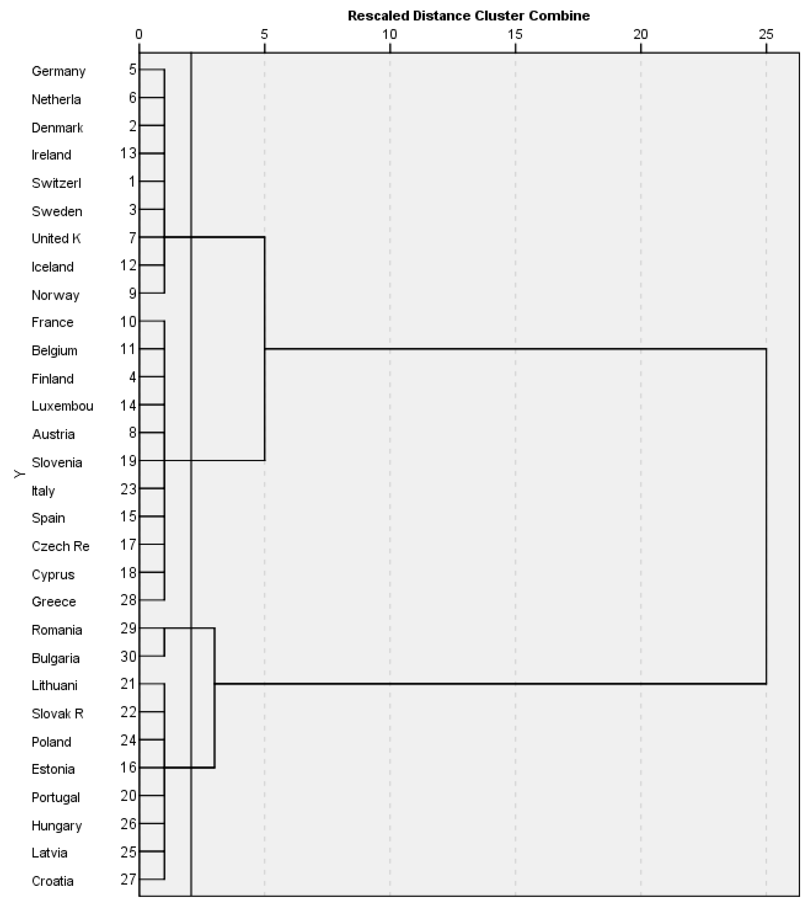
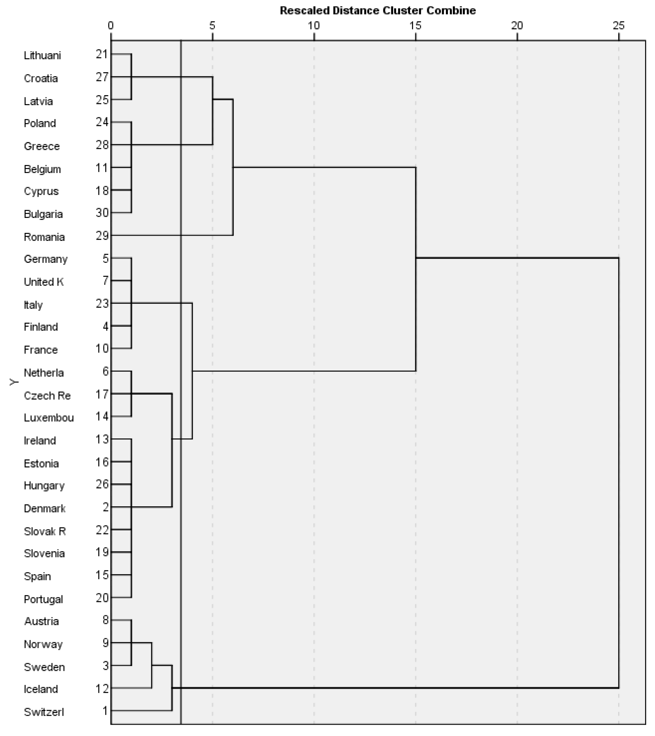
The application of the methodology has led to the classifications of the EU-28 Member States, except Malta, as well as Switzerland, Iceland, and Norway in clusters based on the described research criteria. Thus, based on the HDI values for 2008, 2010, 2012, and 2014 [33], Figure 2 presents the dendrogram obtained using squared Euclidian distance and Ward’s method. This suggests solutions with two-to-four clusters.

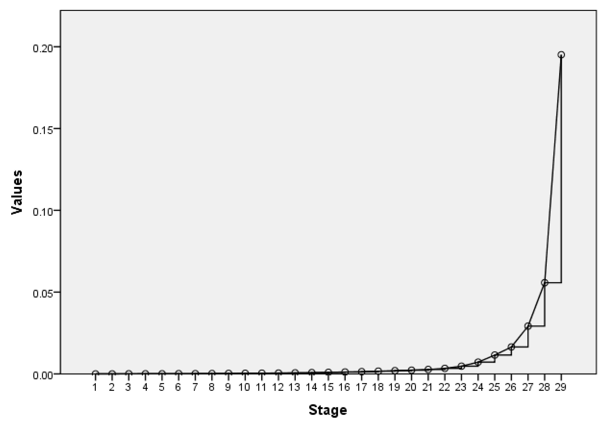
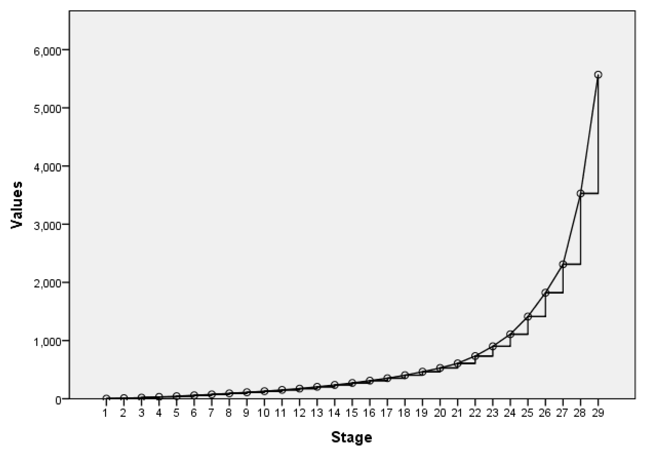
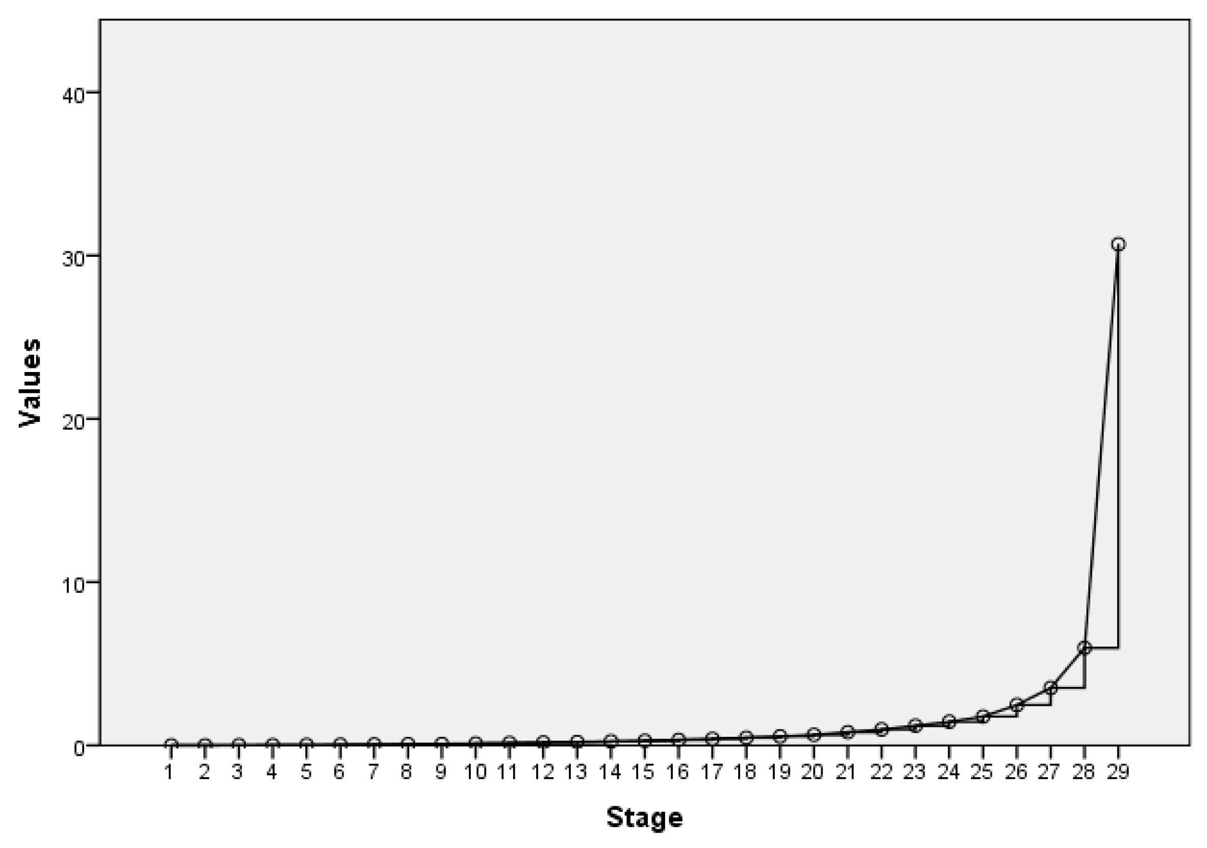
The optimal number of clusters established by parsing the dendrogram—looking for gaps between joining along the axis of the “Rescaled Distance Cluster Combine”—was four. Based on the degree of change in the coefficients in the evaluation table, another approach to validating the hierarchical cluster analysis was performed through the agglomeration schedule coefficients (Figure 3), which represents the amount of heterogeneity we observe in our cluster solution. Agglomeration schedule coefficients help us to decide how many clusters to include in our solution, by displaying the objects or clusters combined at each stage and the distances at which this merger takes place. In Figure 3, the agglomeration schedule coefficients plot shows a large increase in the coefficients after stage 26. Homogenous and distinct clusters are desired, and between-clusters heterogeneity is desired, so the solution with four clusters was chosen. The number of clusters suggested by the agglomeration schedule coefficients is calculated as a difference between the number of cases (30 in our discussion) and the step of elbow according to the plot (26 in this case). The four clusters are presented in

Table 1. Summary statistics.

		Mean	Median	Standard Deviation	Range	Minimum	Maximum
2008	HDI	0.857	0.868	0.041	0.171	0.766	0.937
	EPI	84.63	84.90	5.22	23.60	71.90	95.50
	GCI	4.80	4.70	0.52	1.58	4.03	5.61
	GDP	27,580	25,950	17,330	72,900	5000	77,900
2010	HDI	0.860	0.871	0.041	0.166	0.773	0.939
	EPI	71.02	69.15	8.51	37.20	56.30	93.50
	GCI	4.74	4.59	0.49	1.64	3.99	5.63
	GDP	27,057	25,050	17,916	74,000	5200	79,200
2012	HDI	0.863	0.873	0.041	0.167	0.776	0.943
	EPI	63.97	64.62	5.79	28.35	48.34	76.69
	GCI	4.77	4.62	0.54	1.86	3.86	5.72
	GDP	28,847	24,600	19,989	77,300	5700	83,000
2014	HDI	0.878	0.885	0.041	0.156	0.792	0.948
	EPI	73.36	75.20	7.67	37.15	50.52	87.67
	GCI	4.80	4.63	0.50	1.66	4.04	5.70
	GDP	29,637	24,500	20,262	83,600	5900	89,500

Source: Authors’ computations.

.

The dendrogram in Figure 2 shows that the K_1,HDI cluster relates to the K_2,HDI cluster better than to the K_3,HDI cluster or the K_4,HDI cluster. Additionally, the K_3,HDI cluster relates to the K_4,HDI cluster more than it relates to the other two clusters. This means that the first two clusters (

Table 2. The structure of the clusters determined by HDI values in 2008, 2010, 2012, 2014.

Cluster	Countries Included in Cluster
K1,HDI	Germany, the Netherlands, Denmark, Ireland, Switzerland, Sweden, United Kingdom, Iceland, Norway
K2,HDI	France, Belgium, Finland, Luxembourg, Austria, Slovenia, Italy, Spain, Czech Republic, Cyprus, Greece
K3,HDI	Lithuania, Slovak Republic, Poland, Estonia, Portugal, Hungary, Latvia, Croatia
K4,HDI	Romania, Bulgaria

Source: Authors’ design.

)—containing the richest countries which are also the oldest members of the EU—relates better between themselves than to the other two clusters, containing the poorest countries which are also newer members of the EU.

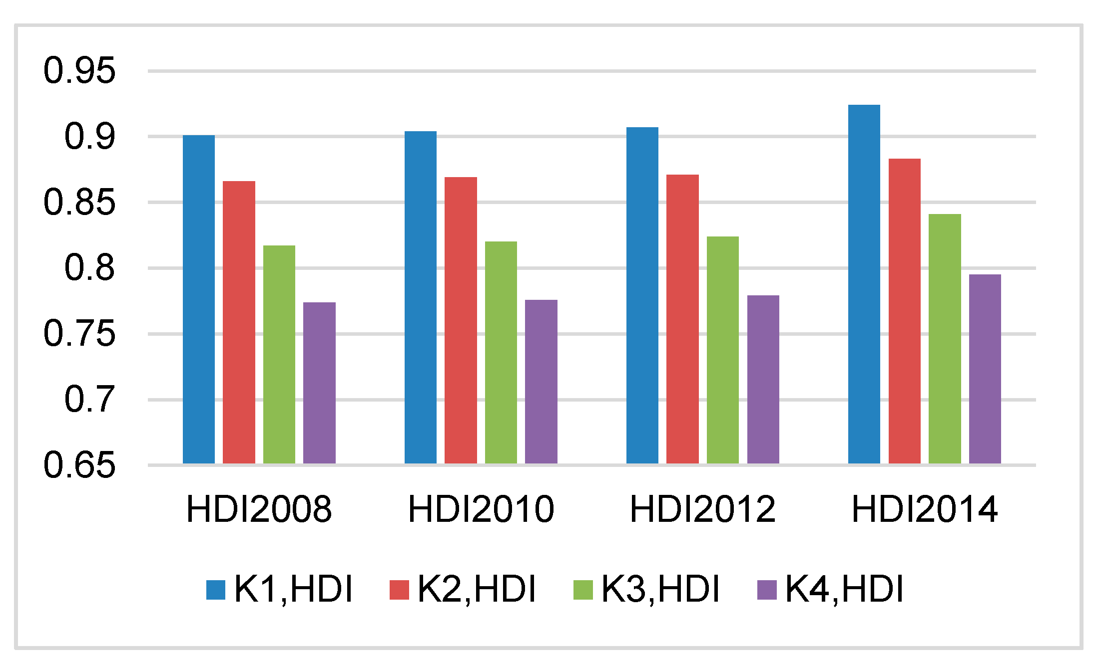
A one-way ANOVA was performed to determine which classifying variables are significantly different between the groups. The detailed results of the analysis are presented in

Table 3. Descriptive statistics for clusters centre (means), HDI values in 2008, 2010, 2012, 2014, and 95% confidence interval for mean.

Cluster		N	Mean	Standard Deviation	Standard Error	95% Confidence Interval for Mean		Minimum	Maximum
						Lower Bound	Upper Bound
HDI2008	K1,HDI	9	0.90089	0.014887	0.004962	0.88945	0.91233	0.886	0.937
	K2,HDI	11	0.86636	0.011360	0.003425	0.85873	0.87400	0.844	0.882
	K3,HDI	8	0.81662	0.010676	0.003775	0.80770	0.82555	0.801	0.832
	K4,HDI	2	0.77350	0.010607	0.007500	0.67820	0.86880	0.766	0.781
	Total	30	0.85727	0.041213	0.007525	0.84188	0.87266	0.766	0.937
HDI2010	K1,HDI	9	0.90389	0.015382	0.005127	0.89207	0.91571	0.886	0.939
	K2,HDI	11	0.86900	0.010991	0.003314	0.86162	0.87638	0.848	0.881
	K3,HDI	8	0.82025	0.009558	0.003379	0.81226	0.82824	0.806	0.830
	K4,HDI	2	0.77600	0.004243	0.003000	0.73788	0.81412	0.773	0.779
	Total	30	0.86027	0.040994	0.007485	0.84496	0.87557	0.773	0.939
HDI2012	K1,HDI	9	0.90733	0.016302	0.005434	0.89480	0.91986	0.890	0.943
	K2,HDI	11	0.87100	0.011866	0.003578	0.86303	0.87897	0.848	0.884
	K3,HDI	8	0.82388	0.010908	0.003857	0.81476	0.83299	0.808	0.839
	K4,HDI	2	0.77900	0.004243	0.003000	0.74088	0.81712	0.776	0.782
	Total	30	0.86320	0.041162	0.007515	0.84783	0.87857	0.776	0.943
HDI2014	K1,HDI	9	0.92356	0.012719	0.004240	0.91378	0.93333	0.908	0.948
	K2,HDI	11	0.88318	0.013688	0.004127	0.87399	0.89238	0.854	0.896
	K3,HDI	8	0.84112	0.012944	0.004576	0.83030	0.85195	0.823	0.863
	K4,HDI	2	0.79500	0.004243	0.003000	0.75688	0.83312	0.792	0.798
	Total	30	0.87820	0.040678	0.007427	0.86301	0.89339	0.792	0.948

Source: Authors’ computations.

, being achieved for the HDI data set referring to all the countries composing the clusters. The mean values confirm the above observation regarding the performance level, in the sense that the highest values of the HDI mean are found in the K_1,HDI cluster for all four years. The Std. Deviation values are increasingly smaller in the K_1,HDI cluster, since 2008 to 2014. This shows that competition is rising among these countries. In the K_4,HDI cluster, the Std. Deviation values recorded a sharp decrease in 2010 compared to 2008, keeping constant since then.

Considering the means of the HDI values, a graphic representation (Figure 4) was made for a clearer emphasis of their evolution on clusters. Thus, for every cluster, the HDI means show rising trends, with strongest increases during 2012 and 2014.

The results of the Test for Homogeneity of Variance are presented in Table 10. As can be observed, all Levene Statistic values are lower than the critical value F_0.05;3;26 = 2.98, leading to the acceptance of the null hypothesis that there are not significant differences between the variances of the data series corresponding to the clusters. Thus, we concluded that the criterion of compactness of the clusters is fulfilled.

The acceptance of this condition referring to the application of the ANOVA methodology being satisfied, the authors used it further to verify the statistical significance of the analyzed variables’ belonging to the clusters. The results are presented in Table 10. The values of F statistics were higher than the critical value F_0.05;4;26 = 2.74, leading to the rejection of the null hypothesis for all four variables, and to the acceptance of the alternative hypothesis: the analyzed variables were statistically significant considering the belonging to clusters.

Countries in the first three clusters belong to the category “Very High Human Development Countries”—HDI values greater than or equal to 0.80, according to the classification made by the United Nations Development Program. In fact, countries belonging to K_1,HDI are all EU countries with HDI values greater than 0.90 in 2014, countries belonging to K_1,HDI and K_1,HDI are countries with HDI values in the range 0.86–0.89 in 2014, and countries belonging to K_4,HDI cluster show HDI values smaller than 0.80, being the only two EU countries included in category “High Human Development Countries”. In the case of Denmark, Sweden, and Iceland, these results could be explained by a high degree of redistribution and the fact that they have the most efficient system of social protection, promoting social inclusion. In the case of Ireland, in our opinion, the education system played a key role; in recent years, many changes have taken place in the education system in Ireland, and a higher access to education at all levels is ensured. Adult education opportunities have also been improved. In the case of Germany, the Netherlands, and Switzerland, employment is the basis of social transfers. Another major issue is a lower inequality of the incomes than in the cases of Ireland and the United Kingdom because of higher spending on social protection in the past. It is noteworthy for the UK that employment is relatively high, showing a downward trend since 2012. For the K_2,HDI cluster, in the case of France, Belgium, Luxembourg, Austria, and Finland, the lower values of HDI could be explained by the fact that the taxation level is high and the granted benefits are low, being dependent on the previous income level. In the cases of Greece, Italy, Spain, and Cyprus, the state has a minimal role in terms of social protection, and family plays a significant role both socially and on the productive plan, while the labor market is highly fragmented and rigid. In the long-term, unemployment rate is especially high among young people, although the social expenditure budget is low. In the case of the Czech Republic, a regulated labor market is to be mentioned. Countries belonging to K_3,HDI cluster have become members of the EU since 2004, unlike those belonging to the K_4,HDI cluster, which have become members of the EU since 2007, the gap remaining still visible. Thus, application of the hierarchical cluster methodology confirms that countries can be grouped as components of traditional economic models.

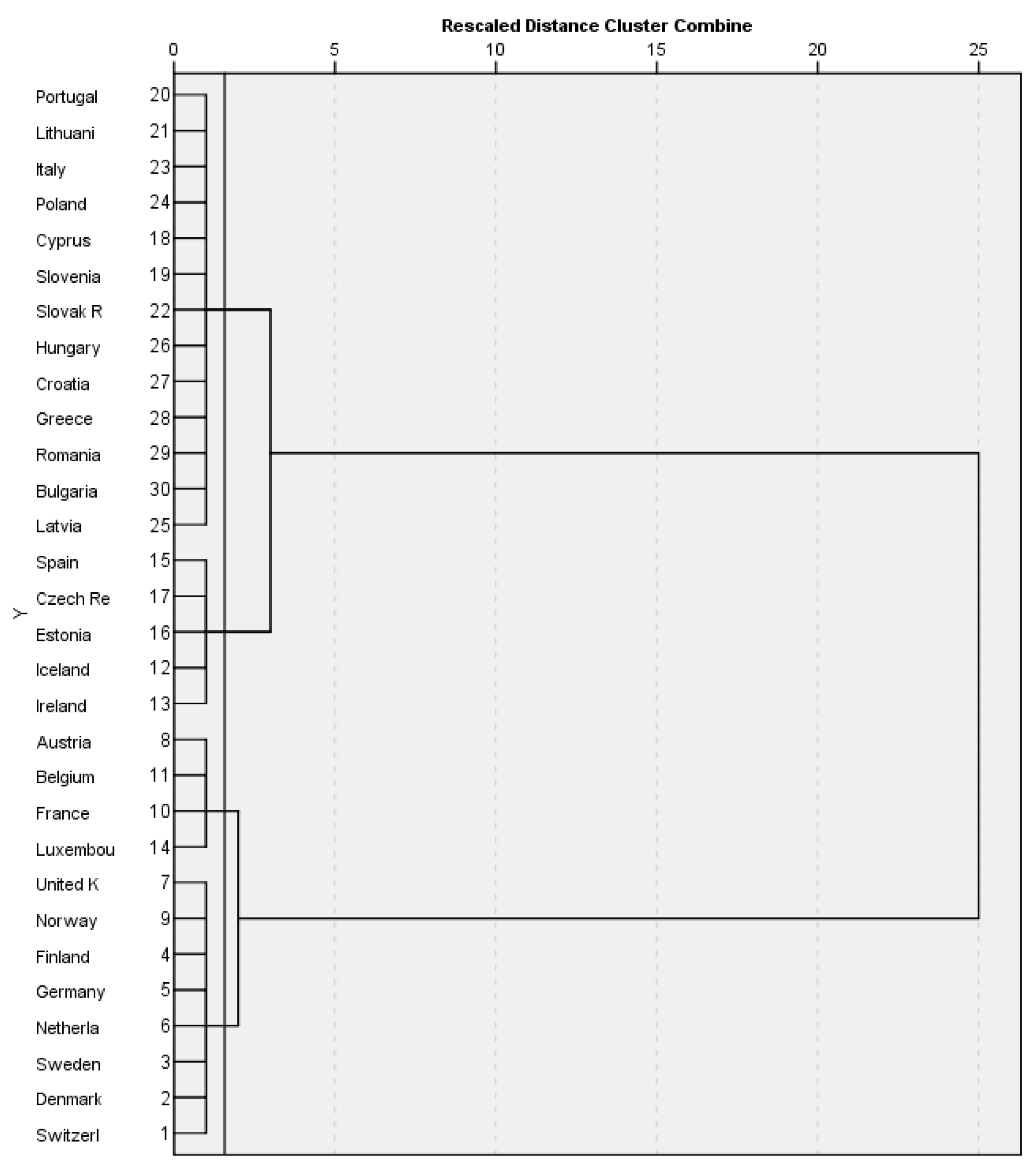
Based on the EPI values for 2008, 2010, 2012, and 2014 [35], Figure 5 presents the dendrogram obtained using squared Euclidian distance and Ward’s method. This suggests solutions with two-to-eight clusters.

The optimal number of clusters established by parsing the dendrogram, looking for gaps between joining along the axis of the “Rescaled Distance Cluster Combine”, was six. The validation of this solution was based on the agglomeration schedule coefficients, in terms of the amount of heterogeneity observed in our cluster solution. Thus, it shows a large increase in the coefficients after stage 24. A solution with six clusters was chosen (Figure 6). Heterogeneous and distinct clusters are desired, so solution A with six clusters was chosen (Figure 6). According to this result, the appropriate number of clusters is six, calculated as a difference between the number of cases and stage of elbow according to the plot.

The six clusters are presented in

Table 4. The structure of the clusters determined by EPI values, in 2008, 2010, 2012, 2014.

Cluster	Countries Included in Cluster
K1,EPI	Austria, Norway, Sweden, Iceland, Switzerland
K2,EPI	Germany, United Kingdom, Italy, Finland, France
K3,EPI	The Netherlands, Czech Republic, Luxembourg, Ireland, Estonia, Hungary, Denmark, Slovak Republic, Slovenia, Spain, Portugal
K4,EPI	Lithuania, Croatia, Latvia
K5,EPI	Poland, Greece, Belgium, Cyprus, Bulgaria
K6,EPI	Romania

Source: Authors’ design.

. According to the dendrogram in Figure 5, the K_2,EPI cluster relates to the K_3,EPI cluster better than to the K_1,EPI cluster, the K_6,EPI cluster, the K_4,EPI cluster, or the K_5,EPI cluster. Additionally, the K_4,EPI cluster relates to the K_5,EPI cluster more than it relates to the other four clusters. This clustering differs from that based on the EPI values, suggesting that the environmental performance has different drivers.

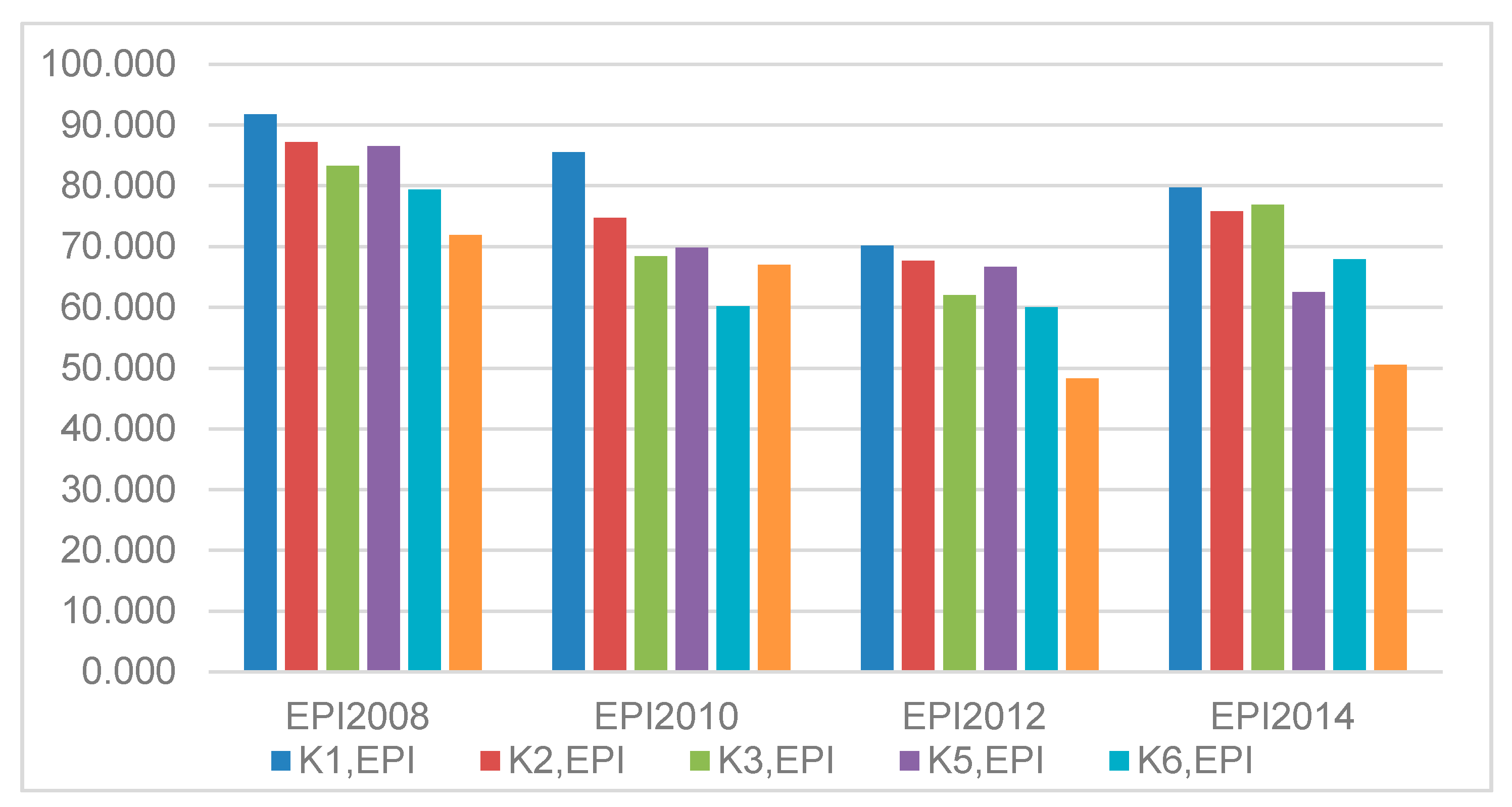
Aiming to determine which classifying variables are significantly different between the groups, a one-way ANOVA was performed. The detailed results of the analysis are presented in

Table 5. Descriptive statistics for clusters centre (means), EPI values in 2008, 2010, 2012, 2014, and 95% confidence interval for mean.

		N	Mean	Standard Deviation	Standard Error	95% Confidence Interval for Mean		Minimum	Maximum
						Lower Bound	Upper Bound
EPI2008	K1,EPI	5	91.7400	3.18009	1.42218	87.7914	95.6886	87.60	95.50
	K2,EPI	11	83.2636	3.02135	0.91097	81.2339	85.2934	76.80	86.30
	K3,EPI	5	87.2000	2.67488	1.19624	83.8787	90.5213	84.20	91.40
	K4,EPI	5	79.3600	0.96073	0.42965	78.1671	80.5529	78.40	80.50
	K5,EPI	3	86.5333	2.11975	1.22384	81.2676	91.7991	84.60	88.80
	K6,EPI	1	71.9000	-	-	-	-	71.90	71.90
	Total	30	84.6300	5.22310	0.95360	82.6797	86.5803	71.90	95.50
EPI2010	K1,EPI	5	85.5600	6.15045	2.75056	77.9232	93.1968	78.10	93.50
	K2,EPI	11	68.3545	2.75912	0.83191	66.5009	70.2081	63.80	73.00
	K3,EPI	5	74.6800	2.08014	0.93027	72.0972	77.2628	73.10	78.20
	K4,EPI	5	60.1800	2.90723	1.30015	56.5702	63.7898	56.30	63.10
	K5,EPI	3	69.8333	2.31805	1.33832	64.0750	75.5917	68.30	72.50
	K6,EPI	1	67.0000	-	-	-	-	67.00	67.00
	Total	30	71.0167	8.50842	1.55342	67.8396	74.1938	56.30	93.50
EPI2012	K1,EPI	5	70.1260	3.90769	1.74757	65.2740	74.9780	66.28	76.69
	K2,EPI	11	61.9973	4.34177	1.30909	59.0804	64.9141	56.09	69.20
	K3,EPI	5	67.6140	1.97479	0.88315	65.1620	70.0660	64.44	69.00
	K4,EPI	5	59.9920	3.28342	1.46839	55.9151	64.0689	56.28	63.47
	K5,EPI	3	66.6767	3.26794	1.88675	58.5587	74.7947	64.16	70.37
	K6,EPI	1	48.3400	-	-	-	-	48.34	48.34
	Total	30	63.9667	5.79462	1.05795	61.8029	66.1304	48.34	76.69
EPI2014	K1,EPI	5	79.7240	4.50028	2.01259	74.1362	85.3118	76.50	87.67
	K2,EPI	11	76.8645	3.63354	1.09555	74.4235	79.3056	70.28	83.29
	K3,EPI	5	75.7900	3.49476	1.56290	71.4507	80.1293	71.05	80.47
	K4,EPI	5	67.9320	3.57705	1.59971	63.4905	72.3735	64.01	73.28
	K5,EPI	3	62.5133	1.41642	0.81777	58.9948	66.0319	61.26	64.05
	K6,EPI	1	50.5200	-	-	-	-	50.52	50.52
	Total	30	73.3600	7.67024	1.40039	70.4959	76.2241	50.52	87.67

Source: Authors’ computations (groups with only one case are ignored in computing the test of homogeneity of variance, cluster K₆).

, based on the EPI data set referring to all the countries composing the clusters. The mean values showed that the highest values were found in the K_1,EPI cluster and the smallest ones in the K_6,EPI cluster for all four years.

Considering the means of the EPI values, a graphic representation (Figure 7) was made for a clearer emphasis of their evolution on clusters. Rankings based on EPI are sensitive to methodological changes, but EPI users can associate clues with peer groups that offer significant comparisons. The major value of EPI is its potential, generated by the values and data underlying the index. EPI was constructed to be used as a starting point for taking environmental action. In the EPI hierarchy, European nations are dominant, with all of the top 10 slots being occupied by European countries. Almost all countries showed an improvement in an EPI score over the review period. Countries that were already at higher performance levels have not improved as much as developing countries. Figure 7 shows a downward trend after 2008 for all clusters, which could be explained by the fact that the environmental issues were left behind the economic and social ones during the crisis period and after that. Some significant increases seemed to appear in the EPI score in 2014 for all six clusters, but these changes mainly result from the improvement made in EPI’s calculus. Thus, the Air Quality and Forest issue include new indicators. Additionally, for the Water issue a new indicator of Wastewater Treatment was added.

The K_1,EPI consists of Austria, Norway, Sweden, Iceland, and Switzerland. Four of these countries (Norway, Sweden, Iceland, and Switzerland) are also part of the K_1,HDI. On the other hand, Lithuania, Croatia, Latvia, and Romania (which are part of the last three clusters, depending on EPI) are also part of the last two clusters, depending on HDI. This seems to show a correlation between environmental performances and social welfare. The second cluster also consists of five countries; namely, Germany, United Kingdom, Italy, Finland, France. Germany and the United Kingdom are also part of the K_1,HDI, and the other three are part of the K_2,HDI. The third cluster contains the largest number of countries: the Netherlands, the Czech Republic, Luxembourg, Ireland, Estonia, Hungary, Denmark, the Slovak Republic, Slovenia, Spain, and Portugal. These countries are in various stages as members of the EU. On one hand, from the point of view of the HDI, they are also members of various categories according to the classification made by the United Nations Development Program. On the other hand, Lithuania, Croatia, Latvia, and Romania—which are part of the last three clusters depending on EPI—are also part of the last two clusters, depending on HDI. This seems to show a correlation between the environmental performances and the social welfare of a country.

The results of the test for homogeneity of variance are presented in Table 10. As can be observed, all Levene Statistic values are lower than the critical value F_0.05;4;24 = 2.78, leading to the acceptance of the null hypothesis that there are not significant differences between the variances of the data series corresponding to the clusters.

The null condition referring to the application of the ANOVA methodology being satisfied, this was used to verify the statistical significance of the analyzed variables’ belonging to the clusters. The results are presented in Table 11. The values of F statistics were higher than the critical value F_0.05;5;24 = 2.62, leading to the rejection of the null hypothesis for all four variables, and to the acceptance of the alternative hypothesis: the analyzed variables were statistically significant, considering the belonging to clusters.

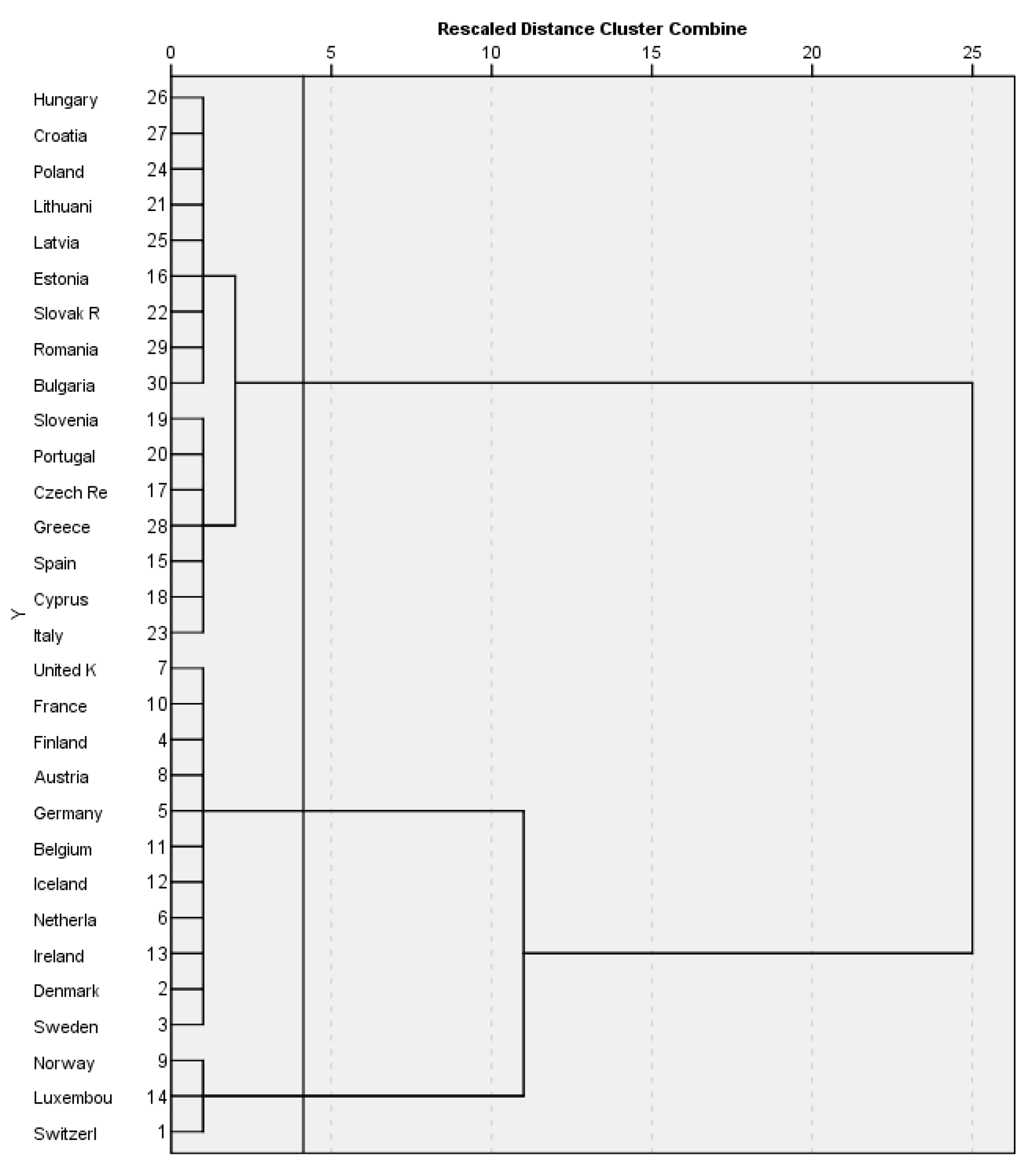
Based on the GCI values for 2008, 2010, 2012, and 2014 [36,37,38,39], Figure 8 presents the dendrogram obtained using squared Euclidian distance and Ward’s method. This suggests solutions with two-to-four clusters.

The optimal number of clusters established by parsing the dendrogram, looking for gaps between joining along the axis of the “Rescaled Distance Cluster Combine”, was four. Based on the degree of change in the coefficients in the evaluation table, another approach to validating the hierarchical cluster analysis was performed through the agglomeration schedule coefficients (Figure 9), which represents the amount of heterogeneity we observe in our cluster solution. Thus, it shows a large increase in the coefficients after stage 26. Homogenous and distinct clusters are desired, and segmentation should also exhibit heterogeneity between clusters, so the solution with four clusters was chosen. The four clusters are presented in

Table 6. The structure of the clusters determined by GCI values, in 2008, 2010, 2012, 2014.

Cluster	Countries Included in Cluster
K1,vGCI	United Kingdom, Norway, Finland, Germany, the Netherlands, Sweden, Denmark, Switzerland
K2, GCI	Austria, Belgium, France, Luxembourg
K3, GCI	Spain, Czech Republic, Estonia, Iceland, Ireland
K4, GCI	Portugal, Lithuania, Italy, Poland, Cyprus, Slovenia, Slovak Republic, Hungary, Croatia, Greece, Latvia Romania, Bulgaria

Source: Authors’ design.

.

The dendrogram in Figure 8 shows that the K_{1, GCI} cluster relates to the K_{2, GCI} cluster better than to the K_{3, GCI} or K_{4, GCI} clusters. Additionally, the K_3,HDI cluster relates to the K_4,HDI cluster more than it relates to the other two clusters. This means that the first two clusters, containing the poorest countries which are also the newest members of the EU, relate better between themselves than to the other two clusters, containing the richest countries which are also older members of the EU.

One-way ANOVA was performed in order to determine which classifying variables are significantly different. The detailed results of the analysis are presented in

Table 7. Descriptive statistics for clusters center (means), GCI values in 2008, 2010, 2012, 2014, and 95% confidence interval for mean.

		N	Mean	Standard Deviation	Standard Error	95% Confidence Interval for Mean		Minimum	Maximum
						Lower Bound	Upper Bound
GCI2008	K1, GCI	8	5.4513	0.13548	0.04790	5.3380	5.5645	5.22	5.61
	K2, GCI	4	5.1100	0.17795	0.08898	4.8268	5.3932	4.85	5.23
	K3, GCI	5	4.8100	0.19609	0.08769	4.5665	5.0535	4.62	5.05
	K4, GCI	13	4.3015	0.16344	0.04533	4.2028	4.4003	4.03	4.53
	Total	30	4.8007	0.51548	0.09411	4.6082	4.9931	4.03	5.61
GCI2010	K1, GCI	8	5.3738	0.15829	0.05596	5.2414	5.5061	5.14	5.63
	K2, GCI	4	5.0850	0.03416	0.01708	5.0306	5.1394	5.05	5.13
	K3, GCI	5	4.6180	0.09680	0.04329	4.4978	4.7382	4.49	4.74
	K4, GCI	13	4.2869	0.17298	0.04798	4.1824	4.3915	3.99	4.51
	Total	30	4.7383	0.49157	0.08975	4.5548	4.9219	3.99	5.63
GCI2012	K1, GCI	8	5.4738	0.14451	0.05109	5.3529	5.5946	5.27	5.72
	K2, GCI	4	5.1575	0.06702	0.03351	5.0509	5.2641	5.09	5.22
	K3, GCI	5	4.6800	0.15281	0.06834	4.4903	4.8697	4.51	4.91
	K4, GCI	13	4.2631	0.18273	0.05068	4.1527	4.3735	3.86	4.46
	Total	30	4.7747	0.54447	0.09941	4.5714	4.9780	3.86	5.72
GCI2014	K1, GCI	8	5.4500	0.12271	0.04338	5.3474	5.5526	5.29	5.70
	K2, GCI	4	5.1475	0.04573	0.02287	5.0747	5.2203	5.08	5.18
	K3, GCI	5	4.6960	0.18022	0.08060	4.4722	4.9198	4.53	4.98
	K4, GCI	13	4.3269	0.16070	0.04457	4.2298	4.4240	4.04	4.54
	Total	30	4.7973	0.50439	0.09209	4.6090	4.9857	4.04	5.70

Source: Authors’ computations.

, being achieved for the GCI data set referring to all the countries composing the clusters. The mean values confirm the above observation regarding the competitiveness level, in the sense that highest values of the GCI mean were found in the K_1,HDI cluster for all four years.

The results of the test for homogeneity of variance are presented in Table 10. As it can be observed, not all Levene Statistic values are lower than the critical value F_0.05;3;26 = 2.98. It was the case of GCI2010. This situation led to the rejection of the hypothesis that there are not significant differences between the variances values of the data series corresponding to the clusters. Thus, GCI2010 appears to not produce significant associations.

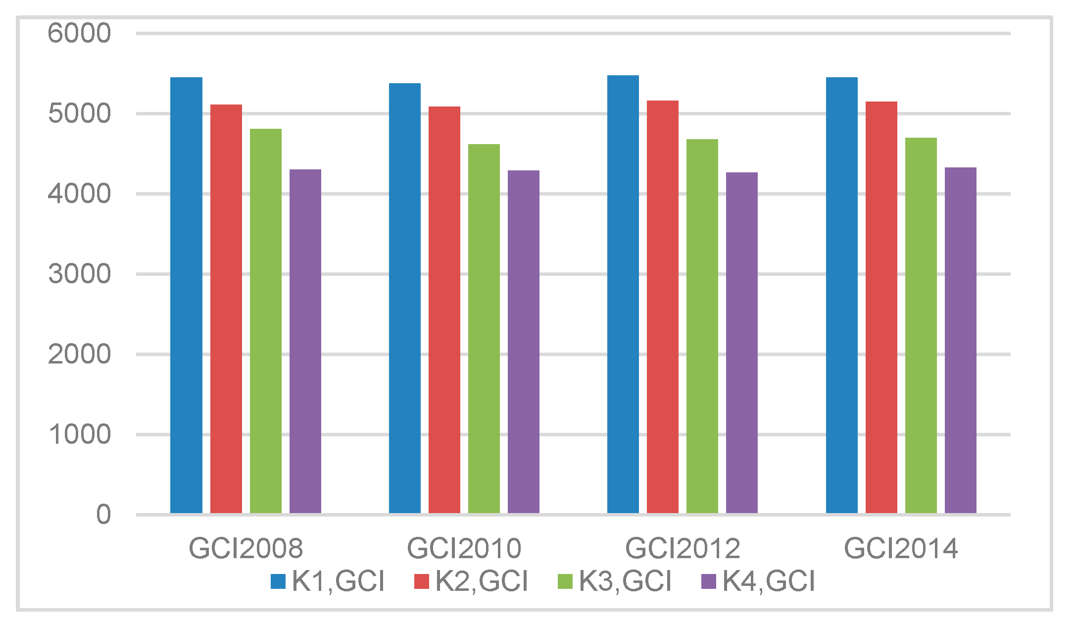
Looking at the means’ evolutions (Figure 10) during 2010, a decrease can be noticed in all cases, followed by a recovery in 2012, except the case of the K_4,GCI, where the recovery appeared only in 2014. This could be explained by a low level of economic resilience in the two countries. This is also supported by the slower recovery of productivity gaps compared to the EU average, according to [51]. These results reinforce the idea that economic growth is unequally distributed in the EU, highlighting the shift of economic activity balance between the older members and the newer ones.

Because the null hypothesis for the Levene’s test was rejected, the F Test was used to test the statistical significance of the analyzed variables’ belonging to the clusters, and the results are presented in Table 11.

The values of F statistics were higher than the critical value F_0.05;4;26 = 2.74, leading to the rejection of the null hypothesis for all four variables, and to the acceptance of the alternative hypothesis: the analyzed variables were statistically significant considering the belonging to clusters.

These results are not in accordance with the ranking provided by the Global Competitiveness Report for 2014–2015. In line with the economic theory of stages of development, this report performed a hierarchy based on the stages of development of the countries, identifying three stages and two intermediary levels. All the countries belonging to the first three clusters, namely, United Kingdom, Norway, Finland, Germany, the Netherlands, Sweden, Denmark, Switzerland, Austria, Belgium, France, Luxembourg, Spain, Czech Republic, Estonia, Iceland, and Ireland, and also six of the countries belonging to the K_4,GCI, namely, Italy, Cyprus, Slovenia, Slovak Republic, Greece, and Portugal, are allocated to Stage 3: Innovation-driven. Five of the countries belonging to the K_4,GCI, namely, Lithuania, Slovenia, Slovak Republic, Hungary, Croatia, and Latvia are in the intermediary stage, namely, Transition from stage 2 to stage 3. Bulgaria and Romania are still allocated to Stage 2: Efficiency-driven.

Based on the GDP values for 2008, 2010, 2012, and 2014 [41], Figure 11 presents the dendrogram obtained using squared Euclidian distance and Ward’s method. This suggests solutions with two-to-four clusters.

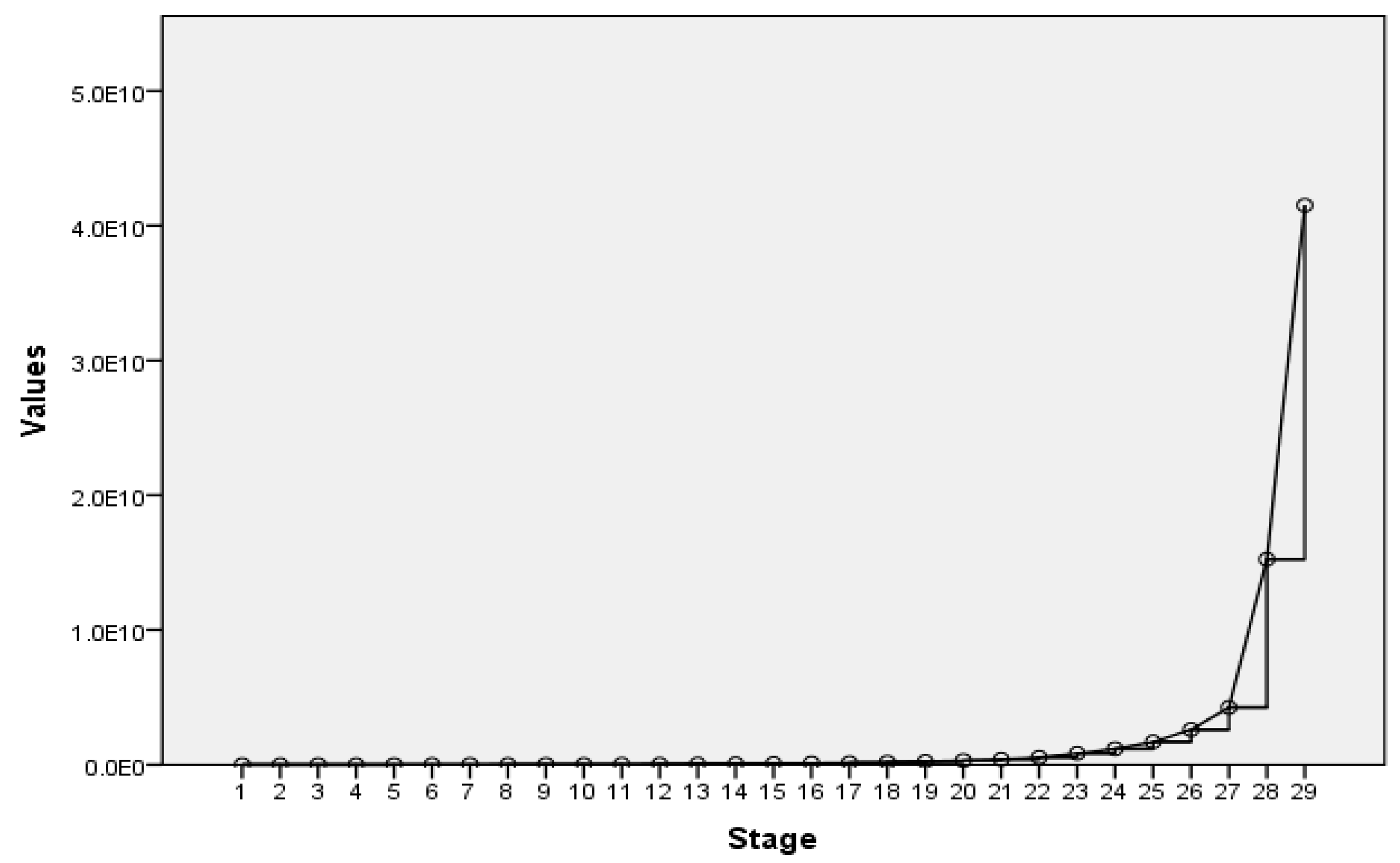
The optimal number of clusters established by parsing the dendrogram—looking for gaps between joining along the axis of the “Rescaled Distance Cluster Combine”—was three. Based on the degree of change in the coefficients in the evaluation table, another approach to validating the hierarchical cluster analysis was performed through the agglomeration schedule coefficients (Figure 12), which represents the amount of heterogeneity we observe in our cluster solution. Thus, it shows an elbow in the coefficients’ plot after stage 27. Homogenous and distinct clusters are desired, so the solution with three clusters was chosen. The three clusters are presented in

Table 8. The structure of the clusters determined by GDP values, in 2008, 2010, 2012, 2014.

Cluster	Countries Included in Cluster
K1, GDP	Norway, Luxembourg, Switzerland
K2, GDP	United Kingdom, France, Finland, Austria, Germany, Belgium, Iceland, the Netherlands, Ireland, Denmark, Sweden
K3, GDP	Hungary, Croatia, Poland, Lithuania, Latvia, Estonia, Slovak Republic, Romania, Bulgaria, Slovenia, Portugal, Czech Republic, Greece, Spain, Cyprus, Italy

Source: Authors’ design.

.

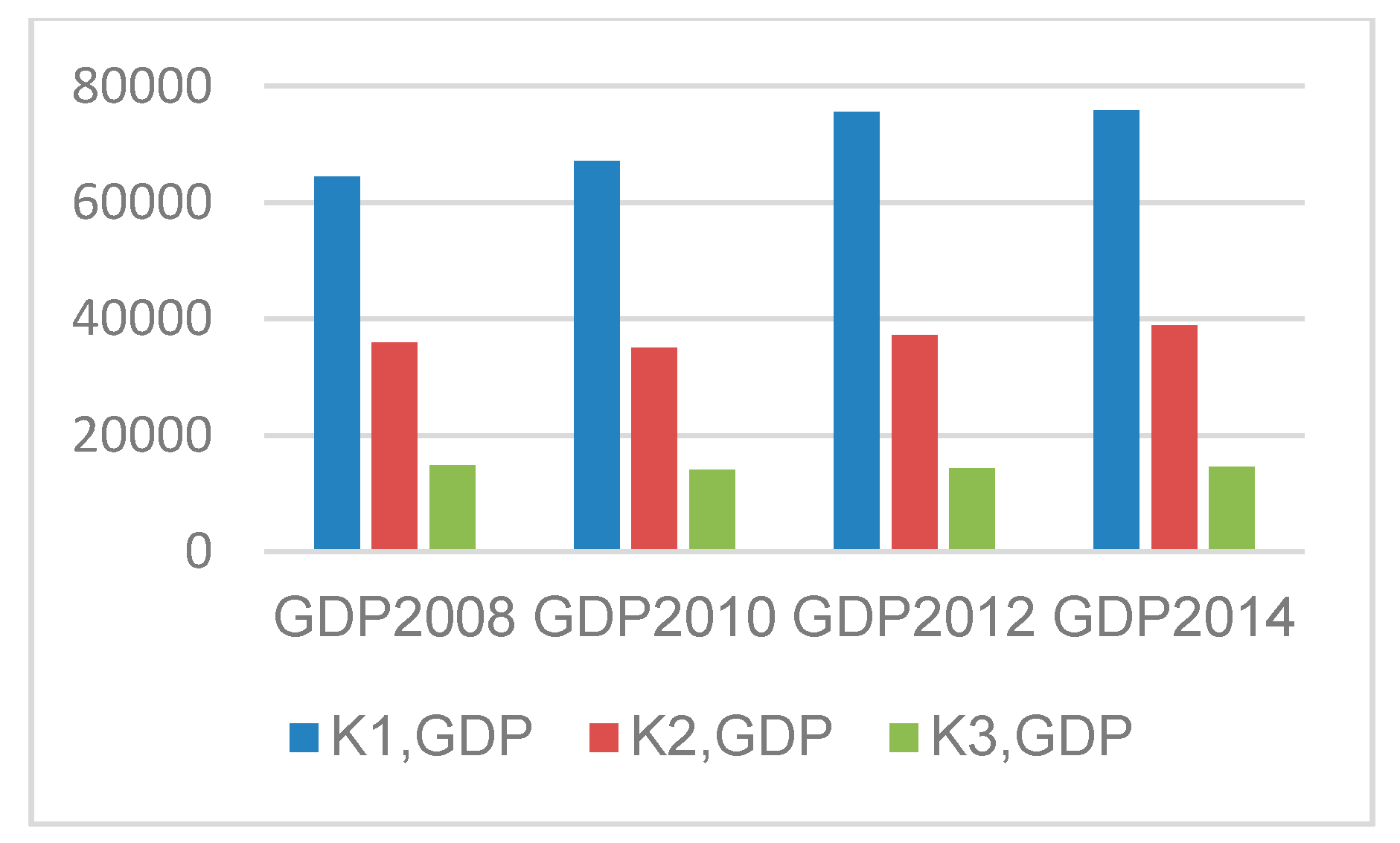
The dendrogram in Figure 11 shows that the K_{2, GDP} cluster relates to the K_{3, GDP} cluster better than to the K_{2, GDP} cluster. This means that the last two clusters, containing the poorest countries which are also the newest members of the EU, relate better between themselves than to the other cluster, containing the richest countries which are also older members of the EU. The K_{2, GDP} and K_{3, GDP} contain the poorest countries which are also the newest members of the EU, except Portugal, Spain, Greece, and Italy, which are older members. This segmentation is strongly in accordance with the economic performances of the countries expressed by GDP as shown in Table 8 and Figure 13. Thus, the GDP mean values in the K_{1, GDP} cluster are almost twice as high as in the K_{2, GDP} cluster, and more than four times higher than in the K_{3, GDP} cluster. In fact, the gaps between K_{1, GDP} cluster and K_{3, GDP} cluster increased during 2008–2012, and started to shrink in 2014.

A one-way ANOVA was performed to determine which classifying variables are significantly different between the groups. The detailed results of the analysis are presented in

Table 9. Descriptive statistics for clusters center (means), GDP values in 2008, 2010, 2012, 2014, and 95% confidence interval for mean.

		N	Mean	Standard Deviation	Standard Error	95% Confidence Interval for Mean		Minimum	Maximum
						Lower Bound	Upper Bound
GDP2008	K1, GDP	3	64,433.3333	14,550.02864	8400.46295	28,289.0585	100,577.6082	49,000.00	77,900.00
	K2, GDP	11	35,981.8182	4303.21233	1297.46734	33,090.8808	38,872.7556	31,000.00	44,000.00
	K3, GDP	7	21,285.7143	4430.36062	1674.51892	17,188.3141	25,383.1145	15,400.00	27,600.00
	K4, GDP	9	9922.2222	2456.00172	818.66724	8034.3722	11,810.0723	5000.00	12,300.00
	Total	30	27,580.0000	17,329.57209	3163.93252	21,109.0314	34,050.9686	5000.00	77,900.00
GDP2010	K1, GDP	3	67,100.0000	11,676.04385	6741.16706	38,095.0991	96,104.9009	55,900.00	79,200.00
	K2, GDP	11	35,009.0909	4277.02105	1289.57037	32,135.7491	37,882.4327	29,200.00	43,800.00
	K3, GDP	7	20,457.1429	4209.06052	1590.87534	16,564.4111	24,349.8746	14,900.00	26,800.00
	K4, GDP	9	9122.2222	2248.76509	749.58836	7393.6684	10,850.7761	5200.00	12,400.00
	Total	30	27,056.6667	17,915.58142	3270.92269	20,366.8786	33,746.4547	5200.00	79,200.00
GDP2012	K1, GDP	3	75,566.6667	9620.98401	5554.67771	51,666.8175	99,466.5159	64,700.00	83,000.00
	K2, GDP	11	37,218.1818	4445.63115	1340.40823	34,231.5662	40,204.7975	31,800.00	45,500.00
	K3, GDP	7	19,657.1429	4200.34012	1587.57934	15,772.4762	23,541.8096	15,400.00	26,700.00
	K4, GDP	9	10,188.8889	2623.18720	874.39573	8172.5287	12,205.2491	5700.00	13,500.00
	Total	30	28,846.6667	19,988.78536	3649.43621	21,382.7315	36,310.6018	5700.00	83,000.00
GDP2014	K1, GDP	3	75,800.0000	12,602.77747	7276.21697	44,492.9652	107,107.0348	64,700.00	89,500.00
	K2, GDP	11	38,909.0909	4302.19817	1297.16155	36,018.8349	41,799.3470	32,300.00	47,000.00
	K3, GDP	7	19,357.1429	4133.54454	1562.33298	15,534.2518	23,180.0340	14,900.00	26,700.00
	K4, GDP	9	10,911.1111	2882.03246	960.67749	8695.7849	13,126.4374	5900.00	15,000.00
	Total	30	29,636.6667	20,262.18634	3699.35217	22,070.6419	37,202.6914	5900.00	89,500.00

Source: Authors’ computations.

, being achieved for the GDP data set referring to all the countries composing the clusters. The mean values confirm the above observation regarding the competitiveness level, in the sense that highest values of the GDP mean were found in the K_{1, GDP} cluster for all four years.

The results of the test for homogeneity of variance are presented in

Table 10. Test for homogeneity of variances.

Levene Statistic Variable	2008	2010	2012	2014
HDI *	0.036	0.597	1.015	0.551
EPI **	0.987 a	2.679 a	2.679 a	0.502 a
GCI ***	0.683	3.295 +	1.044	1.644
GDP ****	4.552 ++	3.006	1.898	3.666 +++

* F_0.05;3;26 = 2.98, solution with four clusters; ** F_0.05;4;24 = 2.78, solution with six clusters; *** F_0.05;3;26 = 2.98, solution with four clusters; ⁺ Significance = 0.036 < 0.05 (rejection of the null hypothesis); **** F_0.05;2;27 = 3.35, solution with three clusters; ⁺⁺ Significance = 0.020 < 0.05 (rejection of the null hypothesis); ⁺⁺⁺ Significance = 0.039 < 0.05 (rejection of the null hypothesis); ^a Groups with only one case are ignored in computing the test of homogeneity of variance. Source: Authors’ computations.

. As can be noticed, not all Levene Statistic values are lower than the critical value F_0.05;2;27 = 3.35, leading to the rejection of the null hypothesis that there are not significant differences between the variances of the data series corresponding to the clusters for the cases of GDP2008 and GDP2014. In the case of GDP2008, in our opinion, the fact that there are not significant differences between the variances can be explained by the heterogeneity of the economies of the EU in 2008, taking into account the fact that the last two members had just joined in 2007. In the case of GDP2014, the level of homogeneity of the clusters depending on GDP could be affected by the recovery of the economic gaps by the new entries.

Thus, Romania has recovered greatly in terms of GDP per capita at purchasing power parity compared to Croatia, the Czech Republic, Slovenia, and Hungary. Although it joined the EU in 2013, Croatia has been going through a period of economic stagnation in recent years, after experiencing a strong recession in 2009–2011. Slovenia, another ex-communist country (as well as Croatia) had a GDP per capita in 2008 of about 11,000 Euros higher than in Romania. In 2014, GDP in Slovenia was 7400 Euros higher than in Romania. Romania has recovered from the gap even in relation to Hungary, from about 4500 Euro to about 3400 Euros. As for Bulgaria, Romania’s advance increased from 700 Euros to 1700 Euros. However, the gap grew with Poland and Lithuania. In comparison with Romania, the GDP in Poland increased by 500 Euros, and the one in Lithuania increased by 600 Euros.

In

Table 11. ANOVA Results.

F Variable	2008	2010	2012	2014
HDI *	98.762	103.716	88.448	86.748
EPI **	17.146	30.033	9.378	21.028
GCI ***	87.031	96.874	105.304	107.279
GDP ****	88.775	125.261	176.042	144.950

* F_0.05;4;26 = 2.74, solution with four clusters; ** F_0.05;5;24 = 2.62, solution with six clusters; *** F_0.05;4;26 = 2.74, solution with four clusters; **** F_0.05;3;27 = 2.96, solution with three clusters. Source: Authors’ computations.

, the statistical significance of the analyzed variables’ belonging to the clusters was tested. The values of F statistics were higher than the critical value F_0.05;3;27 = 2.96, leading to the rejection of the null hypothesis for all four variables, and to the acceptance of the alternative hypothesis: the analyzed variables were statistically significant considering the belonging to clusters.

The four variables were analyzed both individually for each year and for the entire period because we assumed that the economic crisis could generate some effects.

Thus, the maximum value of global competitiveness index was recorded in 2012 for Switzerland (5.72). This evolution can be explained by the fact that GCI measures how efficiently a country uses available resources and the capacity of the state to ensure a high standard of living for its citizens. The economic crisis has determined governments to impose austerity measures that led to falling living standards. The Environmental Performance Index also recorded the maximum value in 2008 in Switzerland (95.5). In contrast, the Human Development Index recorded the maximum value in Norway in 2014 (0.948). This evolution can be explained by the manifestation of increasingly accentuated concern for human welfare within the European Union. The decline was more obvious in 2010 compared to 2012, at almost 17 percent. Unlike these, GDP per capita increased continuously.

An important question was how to decide on the number of clusters to retain from the data. The only significant indicator in hierarchical methods for making this decision is the distance to which the objects are combined. The problem to be solved was what the great distance is. One way to solve this problem was to interpret the agglomeration schedule coefficients. Using this plot, we have searched for a distinctive break (elbow). This information was confirmed by using the dendrogram. Because this distance-based decision rule does not work very well in all cases, it is often difficult to identify where the break actually occurs. This was also the case of the EPI variables, and also the case of GCI variables. The variance ratio criterion was chosen to validate our choices.

4. The Romanian Case

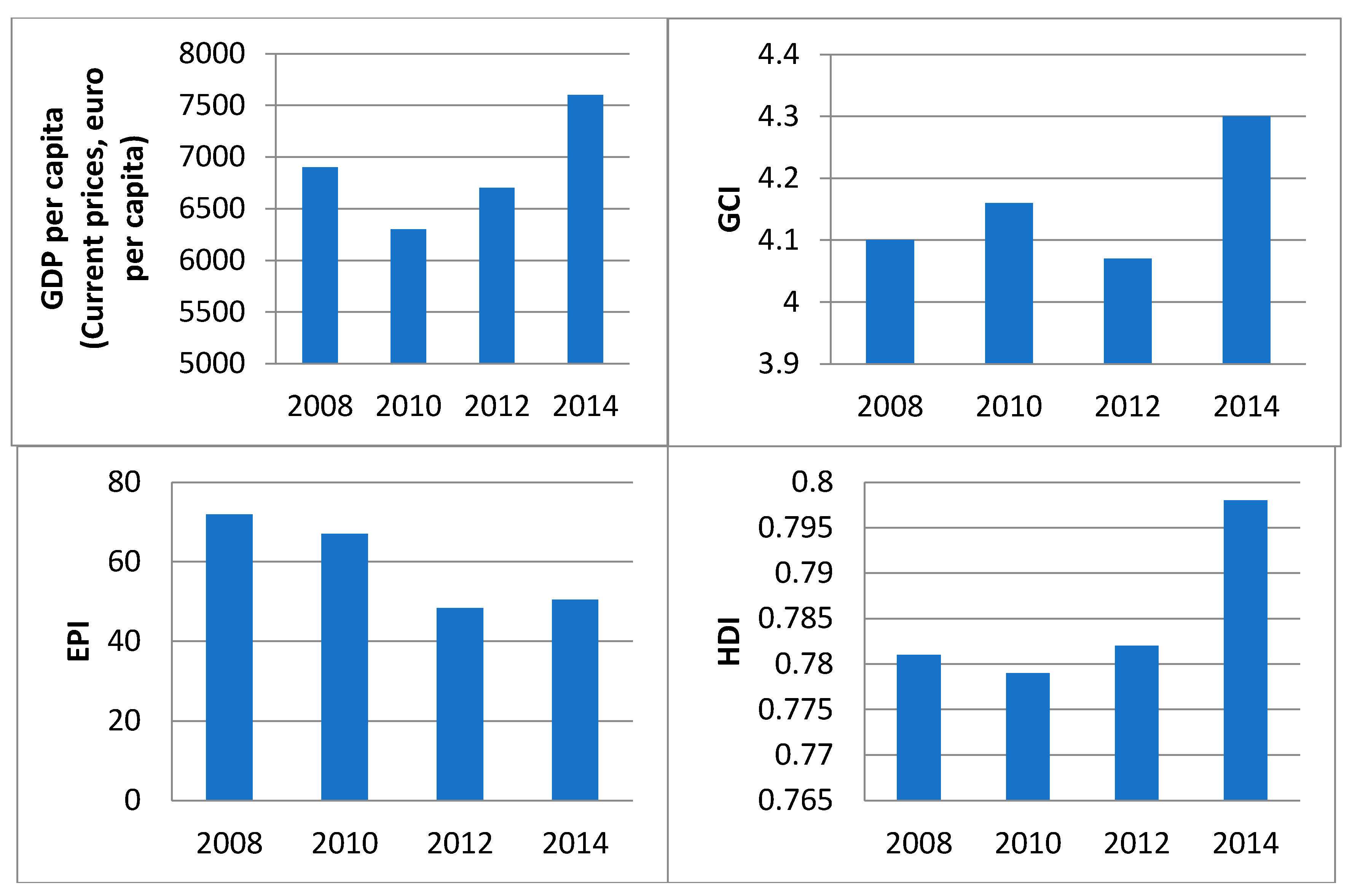
In Romania during 2008–2014, the evolution of GDP per capita showed a general upward trend. Before the crisis, in 2008, Romania had been called the economic tiger of Europe, considering the continuously increasing GDP during 2000–2008. In 2009 there was a dramatic decrease by 7.1% compared to 2008. During 2010–2014, the GDP’s evolution was circumscribed to a process of recovery from recession (Figure 14). In 2011, the Romanian economic system’s recovery began, with the GDP recording an average real growth rate of 1.8% during 2001–2015 [52]. In the period preceding the crisis, a rapid rate of growth was recorded in Romania, driven by domestic demand (consumption and investment). During 2001–2008, domestic demand was averaged about 10.4% per year in real terms, significantly above the growth rate of the real GDP (6.3%). This shows that investment and consumption were covered largely by imports and not domestic production, generating the external imbalance. The rapid growth of consumption and investment was financed and supported by accumulating foreign debt in the private sector and by foreign direct investments. They are a more stable source of funding than the loans, stimulating the potential economic growth of the country. Public expenditure rose rapidly before 2008, fueling an overheating of the economy and leading to deepening imbalances in the private and public sectors. The Romanian economy is poorly structured [53]. However, starting in 2010, the Romanian GDP has continuously grown. The restoration was based on the contribution of industry and services. In terms of uses, final consumption expenditure of public administration, changes in inventories, and net exports have had a positive influence on GDP [54,55,56]. Thus, individual consumption of households and the collective consumption of public administration have decreased. Net exports recorded a more pronounced decline. The growth rate of gross fixed capital formation had a negative effect. In this context, attracting foreign capital is a key issue. In terms of the clusters determined by GDP values, Romania is part of the K_3,GDP together with Bulgaria.

Gross domestic product per capita is not an accurate measure of international competitiveness because elements that are not subject to international competition are included in this variable composition [57].

In Romania in the period under review, the GCI recorded the lowest value during 2012–2013 (4.07). Since 2007, becoming a member of EU has determined a considerable improvement of the competitiveness of Romania. Thus, during 2008–2011, GCI registered an upward trend. Importantly, GCI restarted its upward trend in 2013, reaching a value of 4.30 in 2014–2015 (Figure 14). This evolution was because two of the three main drivers of economic growth (health of the macroeconomic environment and status of the public institutions) have achieved significant progress—in terms of Romania’s organizational capacity and simplifying the operations of markets. However, progress was made shyly and actions were taken, but not for a long time. Aside from strategies, plans, and programs requested by the EU, Romania needs a long-term national competitiveness strategy. Another important factor is linked to the country’s technological capability. Technologization depends directly on new investments. It can be achieved by accessing European funds. Unfortunately, the absorption rate of European funds in Romania is still low. This indicator shows how close the European countries are from the established objectives of the environmental policy of their national governments. In terms of the clusters determined by GCI values, Romania is part of the K_{4, GCI} together with Bulgaria.

According to Figure 14, the EPI’s evolution showed a downward trend during 2008–2012. In 2014, it encountered an upward trend. In accordance with this type of evolution, Romania may be included in the category of developing countries which have improved the EPI score over the last decade. Romania’s case is a complex one. Thus, due to the economic crisis, total greenhouse gas (GHG) emissions had a downward trend (from 123.36 million tons of CO₂ equivalent in 2011 to 118.73 million tons CO₂ equivalent in 2012). Thus, Romania has recorded approx. 30 percentage points above the assumed decrease in GHG emissions for 2020—by 20% compared to 1990. By applying some energy efficiency measures (but also because of the economic crisis), the estimated gross final consumption of energy has a lower value than the forecast of the National Renewable Energy Action Plan (NREAP), which will help increase the share of energy from RES in total energy consumption. In terms of the clusters determined by EPI scores, Romania is part of the K_6,EPI.

In the considered period, HDI has recorded annual growth rates which subsequently reflected the overall growth trend of this indicator. The 2014 HDI value was 0.793 (Figure 14). Analyzing HDI components, life expectancy at birth and GDP per capita had positive annual growth rates. An exception was the period 2011–2012 when GDP per capita (in 2011 PPP $) dropped from 17,071 to 17,068. Mean years of schooling in 2010–2012 increased by 0.1 years per year, but in the last three years, it has remained unchanged at 10.8 years. The situation was worse in the case of Schooling expected years. It has decreased from 14.5 in 2010 to 14.2, and then remained unchanged until the end of the analyzed period. This can be explained by the decline in living standards because of the economic crisis, which generated the amplification of school dropouts. Romania’s overall target for 2025 is to exceed the value of 0.8 of the human development index, currently at 0.785. Thus, only Romania and Bulgaria are not in the “big league” in the EU. In fact, in terms of the clusters determined by HDI values, Romania is part of the K_4,HDI together with Bulgaria.

5. Conclusions

As has been remarked in numerous studies, the measurement of sustainable development has acquired new tools. Sustainable development assessment does continue to attract scientific discussion in the field. Nowadays, achieving sustainable development is essential for boosting economic performance and economic development in contemporary societies. This study also reveals that the ways of measuring competitiveness are different depending on the concept used, using specific economic indicators. What is suggestive, however, is the relative magnitude of the indicators (their change in time or space) and less the absolute level of the indicator.

This development is according to both those stated above and our assumption that sustainable competitiveness is also driven by social factors. They had an increasingly important role, resulting from the continuous growth of the average value of HDI. The economic crisis has forced governments to impose austerity measures that led to falling living standards [58]. Thus, HDI’s evolution can be explained by the manifestation of increasingly accentuated concern for human welfare within the European Union [59,60,61,62,63]. The average EPI score decreased continuously during 2008–2012, which indicates that although all organizations are supposedly concerned about environmental problems, in fact, things are not quite so [63,64,65,66,67]. The inconsistencies between the GDP hierarchy and the HDI one can be explained by the way in which the national income is distributed over time throughout society. During the analysis, clusters were designed based on the role of HDI, EPI, GCI, and GDP in assessment of the sustainable performances of the EU members and also of the possible convergences between them at the level of the EU member states. The indicators used in the analysis generate different clusters. Most overlays occur in the clusters that group countries ranked on top, regardless of the indices chosen for clustering. This type of behavior is typical for countries with strong economies which record performance on all three levels—economic, social, and environmental—and implement consistent development policies [68,69,70,71,72]. Norway and Switzerland are the countries that appear in the first cluster in all four analyzed cases. It is noteworthy that none of them are members of the EU, which allows them to design their policies according to their own interests. Among the EU countries, Sweden is the one that is most often in the leading cluster. The Czech Republic and Slovak Republic are the best placed among former communist countries. Overlaps occur also in the last place of the hierarchy; this is the Romanian case.

Considering the results obtained by the analysis, it can be appreciated that the main objective of this study was achieved, leading to the conclusion that these indices are not able to offer an exhaustive image of the sustainable performances assessment. A new complex indicator could be considered in order to design a convergence model for the EU member states. Such an indicator could help in designing a complex model for the assessment of the sustainable development of a country. It could represent the framework for implementing the best practice models in lower-ranking countries.

References

- Stephen, P.; Brown, D.; Hughes, M. Measuring resilience and recovery. Int. J. Disaster Risk Reduct. 2016, 19, 447–460. [Google Scholar]
- Molyneaux, L.; Brown, C.; Wagner, L.; Foster, J. Measuring resilience in energy systems: Insights from a range of disciplines. Renew. Sustain. Energy Rev. 2016, 59, 1068–1079. [Google Scholar] [CrossRef]
- Daly, H.E. Allocation, distribution, and scale: Towards an economics that is efficient, just, and sustainable. Ecol. Econ. 1992, 6, 185–193. [Google Scholar] [CrossRef]
- Costanza, R.; Cumberland, J.H.; Daly, H.; Goodland, R.; Norgaard, R.B.; Kubiszewski, I.; Franco, C. An Introduction to Ecological Economics; Taylor and Francis Group: Boca Raton, FL, USA, 2014. [Google Scholar]
- Costanza, R.; Patten, B.C. Defining and predicting sustainability. Ecol. Econ. 1995, 15, 193–196. [Google Scholar] [CrossRef]
- Daly, H.E. Toward some operational principles of sustainable development. Ecol. Econ. 1990, 2, 1–6. [Google Scholar] [CrossRef]
- Proag, V. Assessing and Measuring Resilience. Procedia Econ. Financ. 2014, 18, 222–229. [Google Scholar] [CrossRef]
- Rose, A.; Liao, S.-Y. Modeling Regional Economic Resilience to Disasters: A Computable General Equilibrium Analysis of Water Service Disruptions. J. Regul. Sci. 2005, 45, 75–112. [Google Scholar] [CrossRef]
- Costanza, R.; Hart, M.; Kubiszewski, I.; Talberth, J. Moving beyond GDP to measure well-being and happiness. Solutions 2014, 5, 91–97. [Google Scholar]
- Nordhaus, W.; Tobin, J. Is growth Obsolete? In Economic Growth; National Bureau of Economic Research; Columbia University Press: New York, NY, USA, 1972. [Google Scholar]
- Zolotas, X. Economic Growth and Declining Social Welfare; University Press: New York, NY, USA, 1981. [Google Scholar]
- Eisner, R. Extended Accounts for National Income and Product. Am. Econ. Assoc. 1988, 26, 1611–1684. [Google Scholar]
- Daly, H.; Cobb, J. For the Common Good—Redirecting the Economy towards Community, the Environment and a Sustainable Future; Beacon Press: Boston, MA, USA, 1989. [Google Scholar]
- Atkinson, G.; Duborg, R.; Hamilton, K.; Munashinghe, M.; Pearce, D.; Young, C. Measuring Sustainable Development. Macroeconomic and the Environment; Edward Elga: Cheltenham, UK, 1997. [Google Scholar]
- Mäler, K.-G. National accounts and environmental resources. J. Environ. Econ. Resour. 1991, 1, 1–15. [Google Scholar]
- Mäler, K.-G. Welfare indices and the environmental resource base. In Principles of Environmental and Resource Economics: A Guide for Students and Decision-Makers; Henk, F., Landix, G.H., Hans, O., Eds.; Aldershot: Brookfield, UK, 1995; pp. 300–312. [Google Scholar]
- Wackernagel, M.; Rees, W. Our Ecological Footprint: Reducing the Impact on the Earth; New Society Publishing: Gabriola Island, BC, Canada, 1996. [Google Scholar]
- Moffatt, I. An evaluation of environmental space as the basis for sustainable Europe. Int. J. Sustain. Dev. World Ecol. 1996, 3, 49–69. [Google Scholar] [CrossRef]
- Hamilton, K. Green Adjustment to GDP. Res. Policy 1994, 20, 155–168. [Google Scholar] [CrossRef]
- Klasen, S. Growth and Well-being: Introducing distribution-weighted growth rates to reevaluate U.S. Post-War Economic Performance. Rev. Income Wealth 1994, 40, 251–272. [Google Scholar] [CrossRef]
- Hamilton, K.; Atkinson, G. Air pollution and green accounts. Energy Policy 1996, 24, 675–684. [Google Scholar] [CrossRef]
- Jernelöv, A. Swedish Environmental Debt. A Report from the Swedish Advisory Council: Statens Offentliga Utredningar, Sweeden. 1992. Available online: http://agris.fao.org/agris-search/search.do?recordID=SE19930052883 (accessed on 12 November 2014).
- Azar, C.; Holmberg, J. Defining the generational environmental debt. Ecol. Econ. 1995, 14, 7–19. [Google Scholar] [CrossRef]
- Kasimovskaya, E.; Didenko, M. International Competitiveness and Sustainable Development: Are they apart, are they together. A quantitative approach. SBS J. Appl. Bus. Res. 2013, 2, 37–51. [Google Scholar]
- UNDP. Human Development Report 1997; Published for the United Nations Development Programme (UNDP); Oxford University Press: Oxford, UK, 1997. [Google Scholar]
- Ul Haq, M. Reflections on Human Development; Oxford University Press: New York, NY, USA, 1999. [Google Scholar]
- Esty, D.; Levy, M.A.; Kim, C.H.; de Sherbinin, A.; Srebotnjak, T.; Mara, V. Environmental Performance Index; Yale Center for Environmental Law and Policy: New Haven, CT, USA, 2008. [Google Scholar]
- Lober, D.J. Evaluating the environmental performance of corporations. J. Manag. Issues 1996, 8, 184–205. [Google Scholar]
- Epstein, M.J. Measuring Corporate Environmental Performance; IMA/McGraw Hill: San Francisco, CA, USA, 1996. [Google Scholar]
- Wackernagel, M. Shortcomings of the Environmental Sustainability Index. Notes by Mathis Wackernagel, Redefining Progress. 2001. Available online: http://www.antilomborg.com/ESI%20critique.rtf (accessed on 15 July 2016).
- Haberland, T. Federal Environment Agency (Umweltbundesamt), Analysis of the Yale Environmental Performance Index (EPI). Available online: https://www.umweltbundesamt.de/sites/default/files/medien/publikation/long/3429.pdf (accessed on 12 November 2014).
- Bhanu, M.; Raghbendra, J. A Critique of the Environmental Sustainability Index, Australian National University, Discussion Paper. 2003, pp. 1–28. Available online: https://crawford.anu.edu.au/acde/publications/publish/papers/wp2003/wp-econ-2003-08.pdf (accessed on 12 November 2014).
- United Nations Development Programme. The Human Development Report. 2016. Available online: http://hdr.undp.org/en/data (accessed on 15 July 2016).
- Klaus, S.; Michael, E.P.; Jeffrey, D.S. The Global Competitiveness Report 2001–2002. World Economic Forum, 2001; p. 19. Available online: http://citeseerx.ist.psu.edu/viewdoc/download?doi=10.1.1.476.4940&rep=rep1&type=pdf (accessed on 19 November 2014).
- Yale Data-Driven Environmental Solutions Group. The Environmental Performance Index (EPI). Available online: http://epi.yale.edu/data (accessed on 15 July 2016).
- Schwab, K; Porter, M.E. The Global Competitiveness Report 2008–2009; World Economic Forum: Geneva, Switzerland, 2008; pp. 12–17. [Google Scholar]
- Schwab, K. The Global Competitiveness Report 2010–2011; World Economic Forum: Geneva, Switzerland, 2010; pp. 16–21. [Google Scholar]
- Schwab, K. The Global Competitiveness Report 2012–2013; World Economic Forum: Geneva, Switzerland, 2012; pp. 14–19. [Google Scholar]
- Schwab, K. The Global Competitiveness Report 2014–2015; World Economic Forum: Geneva, Switzerland, 2014; pp. 14–19. [Google Scholar]
- Eurostat. Main GDP Aggregates Per Capita nama_10_pc. Available online: http://appsso.eurostat.ec.europa.eu/nui/show.do?dataset=nama_10_pc&lang=en (accessed on 21 April 2017).
- Stuetzle, W.; Nugent, R. A Generalized Single Linkage Method for Estimating the Cluster Tree of a Density. J. Comput. Gr. Stat. 2010, 19, 397–418. [Google Scholar] [CrossRef]
- Ho, R. Handbook of Univariate and Multivariate Data Analysis and Interpretation with SPSS, 1st ed.; Chapman and Hall: Boca Raton, FL, USA, 2006. [Google Scholar]
- Anderberg, M.R. Cluster Analysis for Applications; Academic Press: New York, NY, USA, 1973. [Google Scholar]
- Kaufman, L.; Rousseeuw, P.J. Finding Groups in Data. An Introduction to Cluster Analysis; Wiley: Hoboken, NY, USA, 2005; p. 14. [Google Scholar]
- Rencher, A. Methods of Multivariate Analysis, 2nd ed.; Wiley Publishing: New York, NY, USA, 2002. [Google Scholar]
- Arabie, P.; Hubert, L.J.; De Soete, G. (Eds.) Clustering and Classification; World Scientific Publishers: River Edge, NJ, USA, 1996; pp. 337–453. [Google Scholar]
- Rencher, A.C. Methods of Multivariate Analysis, 2nd ed.; John Wiley & Sons: New York, NY, USA, 2002; p. 499. [Google Scholar]
- Popa, M. Statistică Pentru Psihologia I/O: Analiza de Cluster. 2008, pp. 1–21. Available online: https://www.scribd. com/doc/215080402/Analiza-de-Cluster (accessed on 28 April 2017).
- Cormack, R.M. A review of classification. J. R. Stat. Soc. Ser. A (Gen.) 1971, 134, 321–367. [Google Scholar] [CrossRef]
- Milligan, G.W. Ultrametric hierarchical clustering algorithms. Psychometrika 1979, 44, 343–346. [Google Scholar] [CrossRef]
- Dachin, A.; Burcea, F.C. Schimbări structurale şi productivitate în perioada de criză în România. Cazul industriei. Economie Teoretică şi Aplicată 2013, 20, 118–129. [Google Scholar]
- Guvernul României, Programul de Convergenţă. Available online: http://ec.europa.eu/europe2020/pdf/csr2016/cp2016_romania_ro.pdf (accessed on 27 October 2016).
- Bentoiu, C.; Bălăceanu, C.; Apostol, D. The Characterization of the State and the Evolution of the Romanian Economy in the Years 2000–2010. The Main Statistical Indicators. Romanian Statistical Review. Available online: http://www.revistadestatistica.ro/Articole/2012/art_5en_rrs3_2012.pdf (accessed on 27 October 2016).
- Drăgoi, M.C. The health work force migration: economic and social effects. Farmacia 2015, 63, 593–600. [Google Scholar]
- Andrei, D.R.; Gogonea, R.M.; Zaharia, M.; Andrei, J.V. Is Romanian Rural Tourism Sustainable? Revealing Particularities. Sustainability 2014, 6, 8876–8888. [Google Scholar] [CrossRef]
- Popescu, G.; Boboc, D.; Stoian, M.; Zaharia, A.; Ladaru, G.R. A cross-sectional study of sustainability assessment. Econ. Comput. Econ. Cybern. Stud. Res. 2017, 1, 21–36. [Google Scholar]
- Lall, S. Comparing National Competitive Performance: An Economic Analysis of World Economic Form’s Competitiveness Index; World Development 2001; Queen Elizabeth House: Oxford, UK, 2001; Available online: http://biblioteca.fundacionicbc.edu.ar/images/3/34/Politicas_2.pdf (accessed on 22 October 2016).
- Zaman, G.; Vasile, V. Conceptual framework of economic resilience and vulnerability, at national and regional levels. Rom. J. Econ. 2014, 39, 1–6. [Google Scholar]
- Popescu, G.H. The Relevance of the Right to Work and Securing Employment for the Mental Health of Asylum Seekers. Psychosoc. Issues Hum. Resour. Manag. 2016, 4, 227–233. [Google Scholar]
- Popescu, G.H. Does Economic Growth Bring About Increased Happiness? J. Self-Gov. Manag. Econ. 2016, 4, 27–33. [Google Scholar]
- Swinkels, L.; Xu, Y. Is the Equity Market Representative of the Real Economy? Econ. Manag. Financ. Mark. 2017, 12, 51–66. [Google Scholar]
- Nica, E. The Effect of Perceived Organizational Support on Organizational Commitment and Employee Performance. J. Self-Gov. Manag. Econ. 2016, 4, 34–40. [Google Scholar]
- Svizzero, S.; Clement, T. The Post-2015 Global Development Agenda: A Critical Analysis. J. Self-Gov. Manag. Econ. 2016, 4, 72–94. [Google Scholar]
- Nica, E. Energy Security and Sustainable Growth: Evidence from China. Econ. Manag. Financ. Mark. 2016, 11, 59–65. [Google Scholar]
- Machan, T.R. Commerce and Its Normative Dimensions. Psychosoc. Issues Hum. Resour. Manag. 2016, 4, 7–40. [Google Scholar]
- Nica, E. Employee Voluntary Turnover as a Negative Indicator of Organizational Effectiveness. Psychosoc. Issues Hum. Resour. Manag. 2016, 4, 20–226. [Google Scholar]
- Shin, H.-Y. A Proposal for Incorporating Labor Utilization Frameworks into the Formal Labor Force Statistics. J. Self-Gov. Manag. Econ. 2016, 4, 23–41. [Google Scholar]
- Morales, L.; Andreosso-O’Callaghan, B. Volatility in Agricultural Commodity and Oil Markets during Times of Crises. Econ. Manag. Financ. Mark. 2017, 12, 59–82. [Google Scholar]
- Klosse, S.; Muysken, J. Curbing the Labor Market Divide by Fostering Inclusive Labor Markets through a Job Guarantee Scheme. Psychosoc. Issues Hum. Resour. Manag. 2016, 4, 185–219. [Google Scholar]
- Popescu, G.H. The Role of Multinational Corporations in Global Environmental Politics. Econ. Manag. Financ. Mark. 2016, 11, 72–78. [Google Scholar]
- Subic, J; Vasiljevic, Z.; Andrei, J. The impact of FDI on the European economic development in the context of diversification of capital flows. In Proceedings of the 14th International Business Information Management Association, Business Transformation through Innovation and Knowledge Management: An Academic Perspective, Istanbul, Turkey, 23–24 January 2010; Volumes 1–4, pp. 779–787. [Google Scholar]
- Alexandra, A.; Dorel, D. Approaches on Measuring Sustainable Development in Contemporary World-Beyond Classical Indicators. Annals of Constantin Brancusi; University of Targu-Jiu: Targu-Jiu, Romania, 2016. [Google Scholar]
Figure 1.
Whisker plots for data set. Note: where (a) is HDI, (b) is EPI, (c) is GCI, (d) is GDP Source: Authors’ computations. EPI: Environmental Performance Index; GCI: Global Competitiveness Index; GDP: Gross Domestic Product; HDI: Human Development Index.
Figure 2.
Dendrogram using the Ward linkage method, HDI values in 2008, 2010, 2012, 2014. Source: Authors’ computations.
Figure 3.
Agglomeration schedule coefficients, HDI values in 2008, 2010, 2012, 2014. Source: Authors’ computations.
Figure 4.
Evolution of HDI values on cluster in 2008, 2010, 2012, 2014. Source: Authors’ computations.
Figure 5.
Dendrogram using the Ward linkage method, EPI values in 2008, 2010, 2012, 2014. Source: Authors’ computations.
Figure 6.
Agglomeration schedule coefficients, EPI values in the years 2008, 2010, 2012 and 2014. Source: Authors’ computations.
Figure 7.
Evolution of EPI values on clusters in 2008, 2010, 2012, 2014. Source: Authors’ computations.
Figure 8.
Dendrogram using the Ward linkage method, GCI values in 2008, 2010, 2012, 2014. Source: Authors’ computations.
Figure 9.
Agglomeration schedule coefficients, GCI values in 2008, 2010, 2012, 2014. Source: Authors computations.
Figure 10.
Evolution of GCI values on clusters in 2008, 2010, 2012, 2014. Source: Authors’ computations.
Figure 11.
Dendrogram using the Ward linkage method, GDP values in 2008, 2010, 2012, 2014. Source: Authors’ computations.
Figure 12.
Agglomeration schedule coefficients, GDP values in 2008, 2010, 2012, 2014. Source: Authors’ computations.
Figure 13.
Evolution of GDP values on clusters in 2008, 2010, 2012, 2014. Source: Authors’ computations.
Figure 14.
Evolution of GDP per capita GCI, EPI, and HDI in Romania in 2008, 2010, 2012, 2014. Source: Authors’ computations.