Predicting Energy Consumption and CO2 Emissions of Excavators in Earthwork Operations: An Artificial Neural Network Model


Department of Civil, Environmental and Natural Resources Engineering, Luleå University of Technology, Lulea 97187, Sweden
*
Author to whom correspondence should be addressed.
Sustainability 2017, 9(7), 1257; https://doi.org/10.3390/su9071257
Submission received: 17 May 2017
/
Revised: 26 June 2017
/
Accepted: 12 July 2017
/
Published: 19 July 2017
Abstract
:Excavators are one of the most energy-intensive elements of earthwork operations. Predicting the energy consumption and CO2 emissions of excavators is therefore critical in order to mitigate the environmental impact of earthwork operations. However, there is a lack of method for estimating such energy consumption and CO2 emissions, especially during the early planning stages of these activities. This research proposes a model using an artificial neural network (ANN) to predict an excavator’s hourly energy consumption and CO2 emissions under different site conditions. The proposed ANN model includes five input parameters: digging depth, cycle time, bucket payload, engine horsepower, and load factor. The Caterpillar handbook’s data, that included operational characteristics of twenty-five models of excavators, were used to develop the training and testing sets for the ANN model. The proposed ANN models were also designed to identify which factors from all the input parameters have the greatest impact on energy and emissions, based on partitioning weight analysis. The results showed that the proposed ANN models can provide an accurate estimating tool for the early planning stage to predict the energy consumption and CO2 emissions of excavators. Analyses have revealed that, within all the input parameters, cycle time has the greatest impact on energy consumption and CO2 emissions. The findings from the research enable the control of crucial factors which significantly impact on energy consumption and CO2 emissions.

1. Introduction
Earthwork operations are important activities in building and infrastructure projects, where heavy construction machines are used for excavation, transportation and placement or disposal of materials. These heavy construction machines consume a large amount of energy and have a significant impact on the environment [1,2,3]. Heavy construction machines account for more than 50% of the total emissions from construction operations [4]. According to reports from the National Institute of Environmental Research (NIER) and the Korean Statistical Information Service (KSIS), construction equipment consumes the largest quantity of diesel fuel of all industries in the construction sector in Korea [5], and on-site construction equipment produced 6.8% of the total emissions generated in Korea, with carbon dioxide being a main component of these emissions [6]. In Denmark in 2004, construction machinery accounted for 71% of most fuel use, accounting for 50% of all CO2 emissions produced by the construction industry [7]. Within this industry, excavators are a major contributor to the emissions from heavy construction machines [8]. Consequently, excavation operations dominate in terms of total emissions from construction sites because of the prolonged usage of excavators during construction projects [9]. In an extensive study involving twenty-six types of construction equipment in the United States, excavators accounted for 15% of the total energy consumption and CO2 emissions from construction equipment and machinery [10]. Excavators/backhoes are placed second in the top three contributors to CO2 emissions (26%) for on-site construction in respect of total carbon emissions [11]. A 35% reduction in usage time of excavators leads to a reduction of approximately 15% in excavator emissions, and 10% of the total emissions of on-site construction [9]. Therefore, predicting the energy consumption and CO2 emissions from excavators is critical to mitigate the environmental impact of earthwork operations [12].
Climate change due to greenhouse gas emissions is considered a major environmental issue [13,14]. The largest contributions from human sources comes from burning fossil fuels [15] where the emissions of carbon dioxide (CO2) is considered to be the major component contributing to approximately 60% of the global warming effects [16]. In addition, since the early 1990s, CO2 emissions have been the focus of taxation policies in the industrial sectors in most Scandinavian countries [17]. The Swedish Transport Administration (STA) has recently set the target to have a climate neutral infrastructure by 2045 in an effort to reduce both energy use and CO2 emissions in infrastructure projects [18]. These goals will be transformed into procurement criteria on CO2 emissions that the contractors need to fulfill and be able to estimate, and thus control when construction projects are in the early planning stages.
Despite a number of studies of construction machinery, most of the research has focused on measuring, analysis, or assessing fuel and emissions data based on steady-state engine dynamometer tests [19,20,21], roller dynamometers [22], chassis dynamometers [23] and, more recently, on-board measurements using Portable Emission Measurement Systems (PEMS) [24]. Some of these studies focused on developing quantifiable emission inventory data, such as using PEMS to quantify the emissions factor with respect to time or fuel consumption depending on engine load and duty cycle components [25]. Others focused on measuring, analyzing, and reporting real-world fuel use and emissions of excavators [26], and on determining the emission characteristics of excavators and wheel loaders in China [27]. Some investigated the impact of specific parameters on total emissions such as idle time effects on the fuel consumed and the CO2 emissions of non-road diesel construction equipment [28], and using engine performance data to develop a model for estimating fuel consumed and emissions [29]. PEMS has been proposed as a framework to measure, monitor, benchmark, and possibly reduce the air pollution caused by construction equipment [30]. A portable exhaust emissions analyzer, SEMTECH DS by Sensors, has been used to measure the gaseous exhaust emissions from excavators [31]. Another option has been an estimating tool based on the productivity rate with fuel use rate and emission factors from the EPA’s NONROAD model that can estimate excavator emissions [32]. Similarly, there is an estimation taxonomy for fuel use and pollutant emissions rates of Non-road Construction Vehicles [33], and there is also the ENPROD MODEL for estimating the carbon footprint of heavy duty diesel (HDD) construction equipment [34].
Although most research in this field has recognized the need for emission assessments, procedures for construction equipment assessment remain inadequate, and they have not yet been fully investigated [6]. This is partly due to the limited number of studies of the planning phases in this area [35]. Furthermore, most construction estimators pay little attention to the environmental impact of the machinery that they use [34]. Thus, it is necessary to find a method that can estimate the emissions generated at earthworks sites during the planning phase [36,37,38]. However, for earth-moving operations, no methods have been proposed for early planning stage estimations of the energy use and CO2 emissions of excavators that can be used with limited information. This is largely because, at this stage of the operation, there are insufficiently detailed data regarding the construction process [39]. However, there are considerable general data available in respect of the quantity survey and geotechnical investigations during the pre-planning stage of construction projects. These data include parameters such as excavation depth, density of material excavation, bucket payload, default cycle time and horsepower for available excavators, and this information can be used as a primary data source to predict the hourly energy consumption and CO2 emissions of excavators. Therefore, it becomes less expensive to consider the environmental impact at an earlier stage of construction projects [39,40] where available alternatives can be examined and the best selected.
The aim of this study was to develop a model that can help planners predict, during the early planning stages, energy consumption and CO2 emissions from excavators used in earthworks operations, thereby overcoming the problem of the shortage of detailed information from the construction process. In addition, the model would be able to indicate which factors have large impacts on the energy and CO2 emissions from among all of the model’s input parameters, and provide insight into the relative importance of the output of the model for each of them (i.e., energy and emissions). This would then allow planners to compare different alternative excavators in order to reduce the likely CO2 emissions from the construction work. The proposed model is based on artificial neural networks (ANN), and the study puts forward a mathematical formula for predicting the environmental impact of excavator operations based on the operational characteristics for different excavator models and the parameters of the earth excavation. The results from a multivariate linear regression (MLR) analysis of the same input and output parameters are compared with the results of the proposed ANN model, thus demonstrating the efficiency of the ANN model as a prediction formula. The model’s output can help planners to estimate the energy consumption and CO2 emissions of the chosen excavators based on digging depth (Dp), cycle time (Tc), bucket payload (Bp), bank density of excavation materials (Bd), and horsepower of excavator engine (Hp). In addition, planners can easily employ the results of the proposed model using an Excel spreadsheet, Matlab, or any other computational program, depending on their preference.
This paper is organized as follows. First, in Section 1, the introduction explains the relevance and importance of this study, including related literature and models for assessing the CO2 emissions of construction equipment, the current knowledge gap, and the contribution of the study. Section 2 describes the methodology for the proposed models and data generation, Section 3 contains results and discussion and, in the final section, the conclusions, limitation and future research directions are discussed.
2. Methodology of the Proposed Model for Forecasting the Energy Use and CO2 Emissions
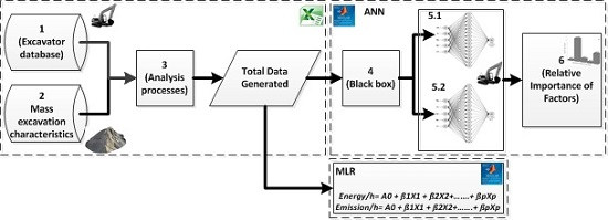
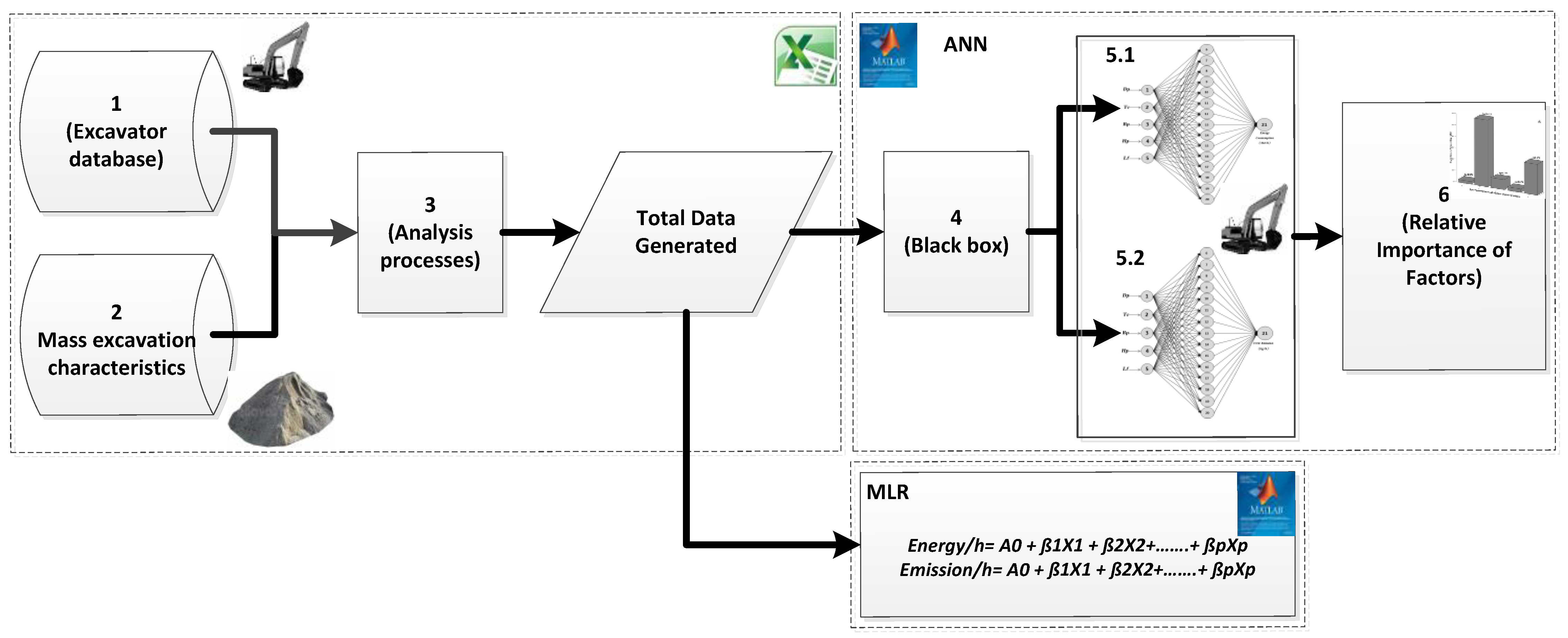
The method used in this research included the steps shown in Figure 1 where the process flows from the start point to production of the final prediction formula. Each step is described in the following (Section 2.1, Section 2.2, Section 2.3, Section 2.4 and Section 2.5).
2.1. Extraction of A Database Based on the Excavator Manufacturer’s Handbook
Typically, an artificial neural network needs a huge database that can be used for building, training and testing it in order to produce a good prediction formula. The basic excavator database was extracted from the Caterpillar handbook 42.0 that covered twenty-five models of excavator [41], as shown in Table 1. The selected excavators were divided into several groups based on the nature of the types of digging recommended for each specific excavator model in the handbook. In addition, duty cycles of excavators were used in the analysis of digging the earth from cutting level to loading onto a truck.
2.2. Collecting Mass Excavation Characteristics of Different Types of Earth
The characteristics of earth excavation (i.e., density, swell factor, and load factor) were investigated using inventory information for three groups of earth (i.e., decomposed rock-packed earth, sand/gravel, and hard clay), according to the recommended use for the excavator models selected (see Table 1). The bulk and loose densities of the selected types of earth depend on the type of earth, digging depth and other geotechnical properties for each layer of excavation.
2.3. Generating the Excavator Database Using Different Characteristics of Mass Excavation to Produce the Input Data for the ANN Model
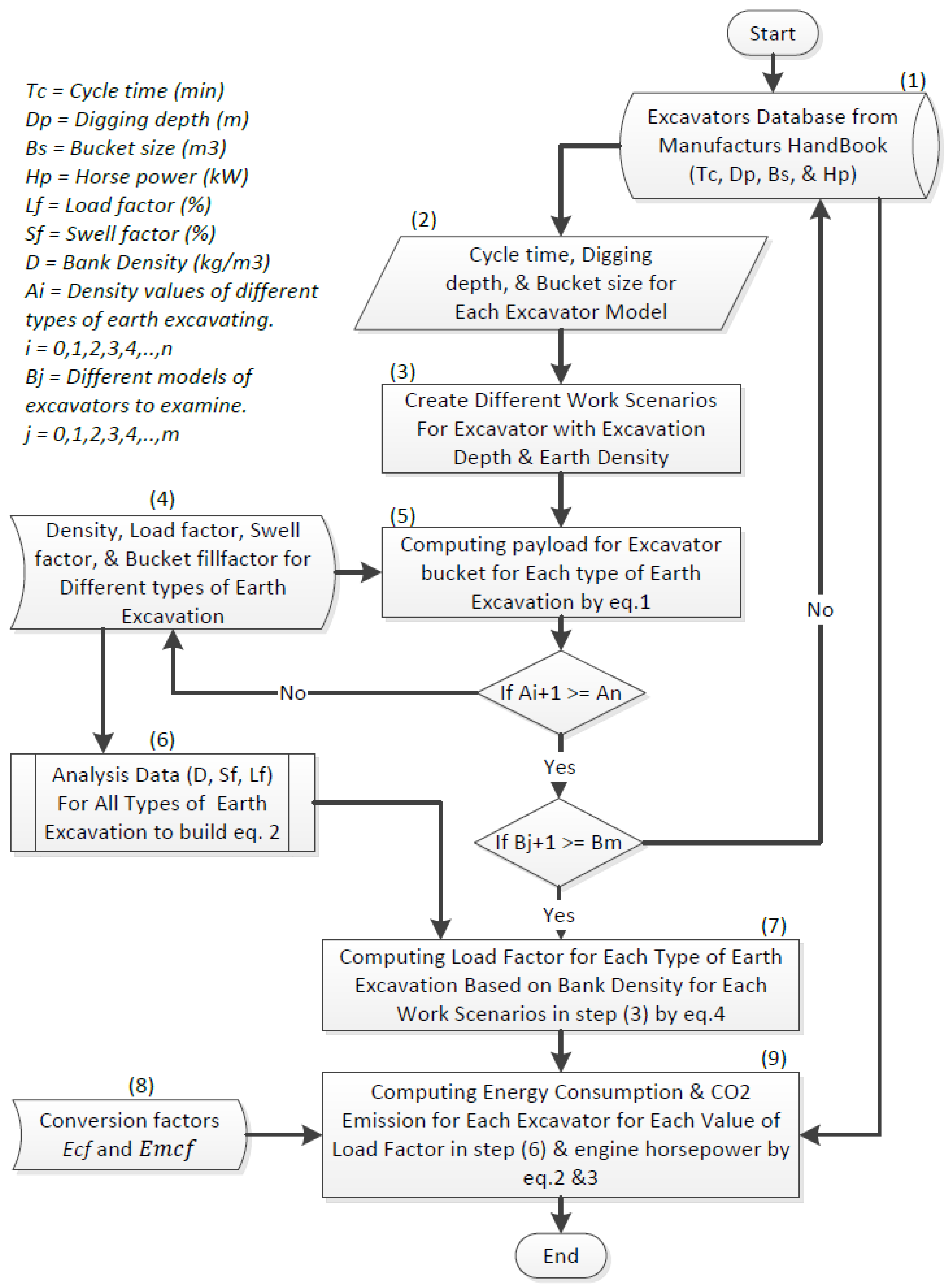
To generate a sufficiently large dataset for the excavator database, it was necessary to include a wide range of variables related to an excavator’s work and the different job conditions and requirements. For each analysis iteration cycle, each excavator type was tested for different scenarios, including different soil types (St), digging depths (Dp), bucket sizes (Bs), bucket payloads (Bp), cycle times (Tc), load factors (Lf), and the engine horsepower of the excavator (Hp). For example, with different types of earth excavation (e.g., packed earth, sand, gravel, and hard clay), each type has various values of earth density, and these values can be put into ranges as shown in Table 1, and then tested for different digging depths with a different bucket size and fill factor for each depth. To illustrate this, Equation (1) was used to calculate bucket payload based on bucket size (Bs) for each model of excavator, together with bucket fill factor (Bf), with a range of 0.65 to 1.1 (see Table 2), and based on the type and density of material being excavated and its shape when loaded in the bucket.
where Bp is the bucket payload representing the actual volume (m3) of material hauled by the excavator bucket (also referred to as heaped bucket capacity); Bs is the design volume (m3) of the excavator bucket (also referred to as struck bucket capacity); and Bf is the percentage of materials actually carried in respect of the excavator bucket’s available volume [41]. An extensive analysis procedure was undertaken, using Excel, to test twenty-five models of Caterpillar excavator with sixteen different values of bucket size within the group’s range, with four different values of bucket fill factor for each one, and different values of load factor based on different density values for each type of earth to be excavated. This analysis led to the production of 5092 rows of data in the database (i.e., each row has a unique set of values), each row having five columns. The final results of this analysis can be expressed as a matrix (with a dimension of 5092 × 5) in order to provide the input matrix for the ANN model. In addition, an energy consumption and CO2 emissions database for each operational scenario of the excavators was created based on the principle equation from Filas 2002 [42]. This approach was proposed in order to estimate fuel consumption, relationships between fuel specifications, load factor (decimal), and engine horsepower (kW) for each excavator’s operational scenario. Equations (2) and (3) can be used to generate energy and emissions (CO2), and also to provide the output database matrices for the ANN and MLR models (with dimensions of 5092 × 1) for each of the energy and CO2 emissions outputs.
where Ed and Emd are, respectively, the energy consumption (MJ/h) and CO2 emissions (kg/h) of the excavator. SFC is specific fuel consumption (0.22 kg/kW h) [43,44], to be set to a suitable value for engines with power in the range 28.8 to 370 kW [43]. Hp is the horsepower of the excavator engine (kW), which represents the maximum power level designed for the excavator engine [45]. Ecf is a conversion factor for the energy of each liter of diesel fuel (36 MJ/L) [46]. ρfuel is the specific gravity of the diesel fuel to be consumed (0.85 kg/L) [47,48,49,50,51,52], ranging between 0.83 and 0.87 kg/L. Emcf is a conversation factor for the carbon dioxide (CO2) of each liter of diesel fuel (2.6569 kg CO2/L) [53]. Lf is the engine load factor (decimal). The engine load factor is greatly affected by the usage patterns of the NONROAD engine [45], and typically this has a range of values depending on engine type and level of utilization [42]. However, this parameter was developed to identify the practical average proportion of engine rated horsepower used, based on work conditions, to take into account the effect of both idle and partial load situations when the machine is being operated [54]. Load factor values are used in Equations (2) and (3) to generate an energy and GHG emission database for the excavators, based on the approach mentioned by [35] in respect of terms described in the manufacturer’s handbook [41], and as described in [55,56], which refer to the density of the excavated material as “bank density”. Thus, a load factor database with material density values (i.e., bank density) was compiled from different sources, and this was then clustered based on three categorized groups, as shown in Table 1. Consequently, forty-two values of load factor with their density values were processed and analyzed using a first degree of exponential algorithms by fitting curve regression analysis to find an acceptable relationship between the two variables (see Equation (4)).
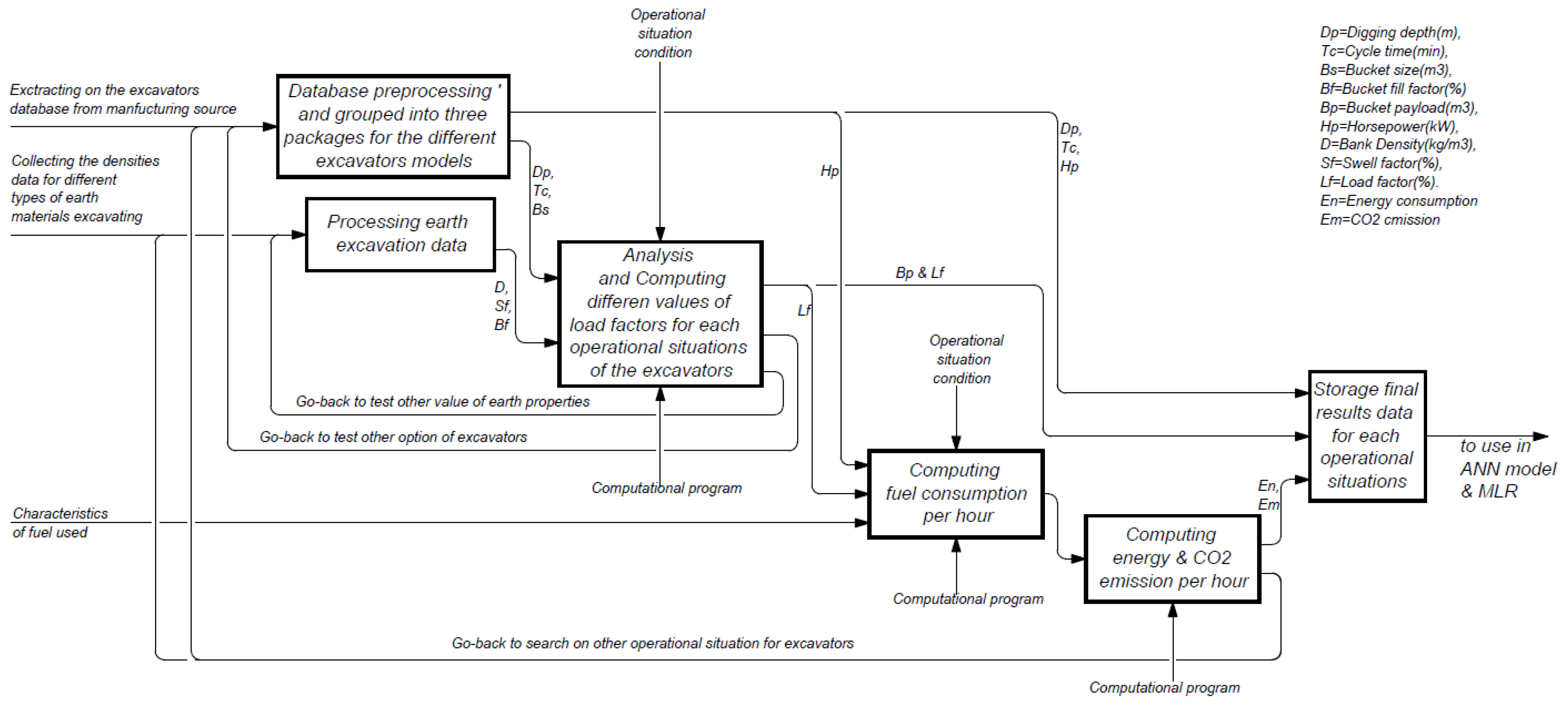
where BD is the bank density (kg/m3) (i.e., the material density in its natural state before disturbance, either in place or in situ). The load factor formula is considered a good representation of the relationship between the densities and load factor based on a goodness of fit report that shows values for R-square of 0.9342, a minimum error of 5.7073 × 10⁻⁴, and a maximum error of 0.1292 for specific values of bank density (in the range 960–2415 kg/m3) and load factor (0.15–0.91). Figure 2 shows the flowchart for the generation of training data sets for the ANN model. Figure 3 shows an integrated definition for function modeling (IDEFO), which represents a simplified process for generating the energy consumption and CO2 emission data of excavators used for earth-moving in construction projects. Table 2 shows the boundary conditions and range limits applied in order to test and analyze various characteristics for excavators related to earth type, thus generating a very large database.
2.4. Designing the Predictive ANN Model with Forwards/Backwards Propagation Learning Algorithms
Building an ANN model requires the predetermination of a preliminary design that can address three points. First, a decision has to be made regarding the number of parameters that can be utilized as input to the number of nodes in the input layer. Following on from the final database that resulted from the analytical processes carried out in Section 2.3, five main parameters associated with the excavator operating cycle were determined as the input parameters for the ANN model with five nodes at the input layer. These parameters represented digging depth (Dp), total cycle time (Tc), bucket payload (Bp), horsepower of the excavator engine (Hp), and load factor (Lf). A second issue is that there should be no rule applied to determine the number of hidden layers in the ANN [57] since using more than one hidden layer can be considered to produce more filtering and weights modification of the ANN’s output [58]. Despite this, one hidden layer is used by most researchers for predicting objectives [59,60,61], this may be problematic for the expression of the final prediction formula, as complicated weightings result when there are many hidden layers [61]. A common practice for determining the number of nodes in the hidden layer is to use trial-and-error or experimentation [59] because there is no fully proven theoretical or algorithmic procedure to determine the nodes in the hidden layer [57,59,62]. In addition, investigative studies of ANNs have shown that the number of hidden layers has no significant effect on prediction performance [59]. In this study, one hidden layer was used in each prediction model (energy consumption and CO2 emission).
According to [57,58,59,60,61], trial-and-error is used to select the optimum number of hidden nodes that meets a minimum value of mean square error for the performance training and testing data subsets in the proposed ANN model. The data for the 5092 cases generated by analysis of the operational characteristics for excavators was divided into two parts: the training set and the testing set. There are no accepted mathematical rules for determining the size of the dataset to be used for training and testing, and the number of training cycles or iterations is almost always decided on by rule of thumb, based on experience and trial-and-error, in order to reach a minimum percentage value of mean square errors [35,63]. Therefore, trials with various sizes of training and testing databases, created from the whole database, were carried out using 75–93% and 25–7%, respectively, of the data for the training and testing database subsets in both ANN models (see Table A1 and Table A2). Perception Multilayer (PML) networks, a backward propagation learning method based on the Levenberg–Marquardt algorithm, were used for the training data in the neural network. Here, a multi-layer feed forward and backward propagation using a supervised learning technique was implemented with a sigmoid activation function to develop and train the neural network. The procedure for data processing inside an ANN model can be divided into three parts. The first part involves using training subset data to update the weight connections in the network layers using backward propagation at the training stage. The second part, in parallel with the learning process, uses the testing subset to identify the responses of the designed neural network to data that do not form part of the training data, but which are a part of the whole dataset and within its boundaries. In the third part, the neural network utilizes data examples that do not belong to the other two subsets (i.e., training and testing) to produce a validation data subset that provides a final indication of model acceptability and validity. In this study, several trials were carried out in order to select an optimum design for the nodes in the hidden layer, and for the size of the training and testing data subsets. Table A1 and Table A2 in the Appendix show the main results for the best seven cases of hidden nodes after 42 trials on various subset sizes selected for both of the ANN models.
The optimum combination figure from among the best forty-two trials of the ANN model running the training and testing data subsets was found to be 40. This was based on the minimum value of mean square error for the training data subset, which is considered the essential criterion to represent the best performance for the backward propagation learning method used for the ANN model adopted to select the best combination [63]. In addition, the value correlation coefficient (R) is considered more useful for comparing appropriate models with the different number of predictors for ANNs [58]. R also represents the correlation value between the prediction and the actual output value of a neural network [63]. However, R is a poor measure when it is zero or near zero (which indicates a lack of a relationship between the predicted and actual output of the ANN model) [63]. Thus, a value for R of 1 (or near 1) is seen as a robust indicator of good relevance between the predicted and the actual output [63]. Therefore, 0.9 is a minimum value of R in order for the neural network model to be considered a good model, one that represents a perfect fit between the target and actual output [63].
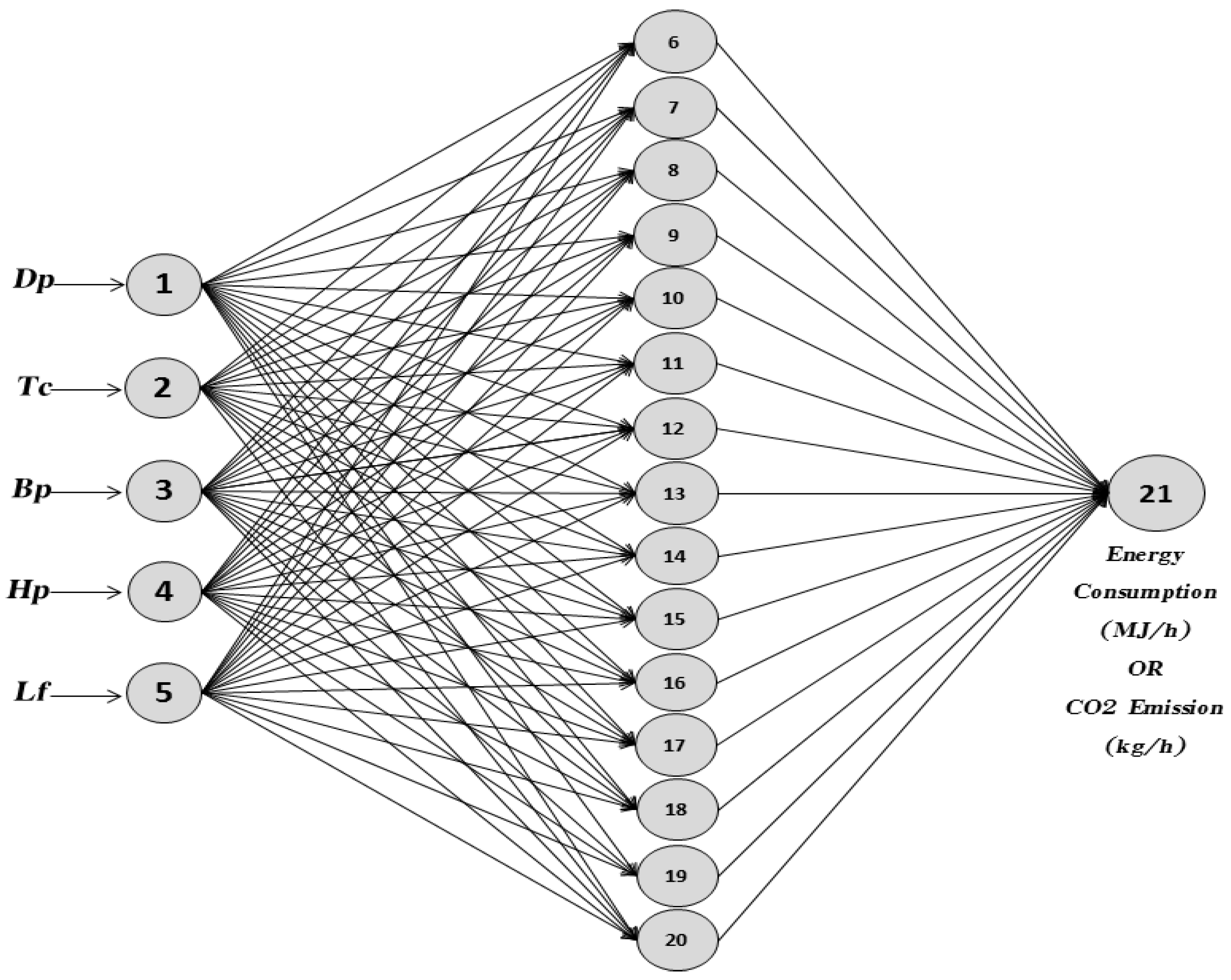
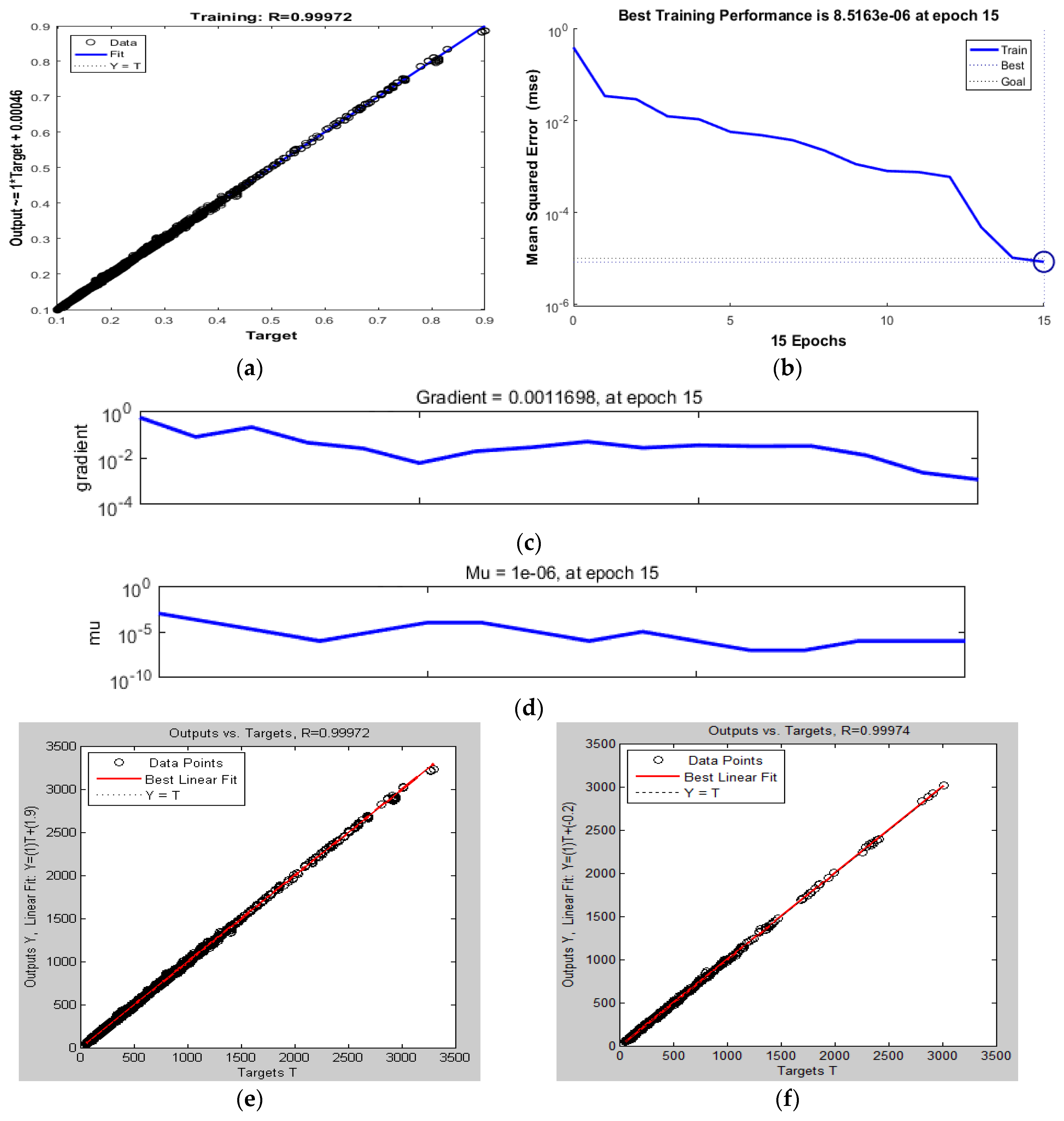
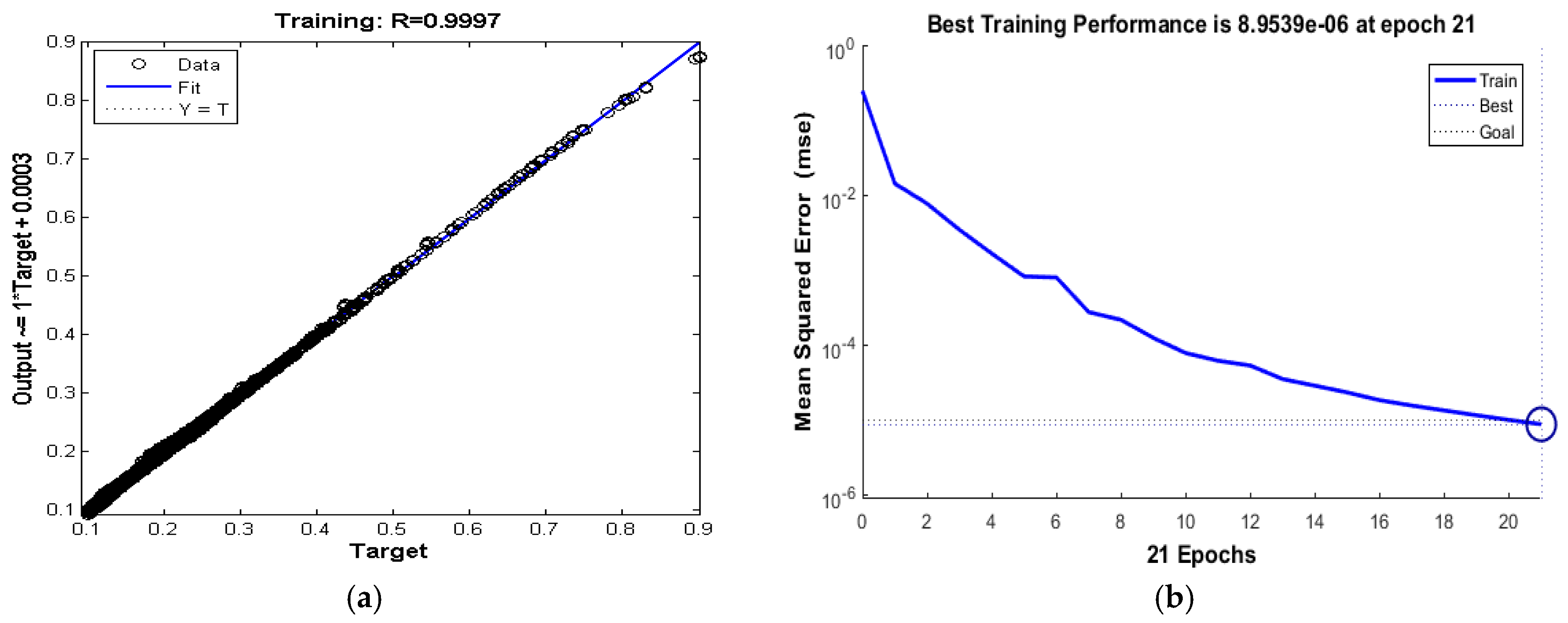
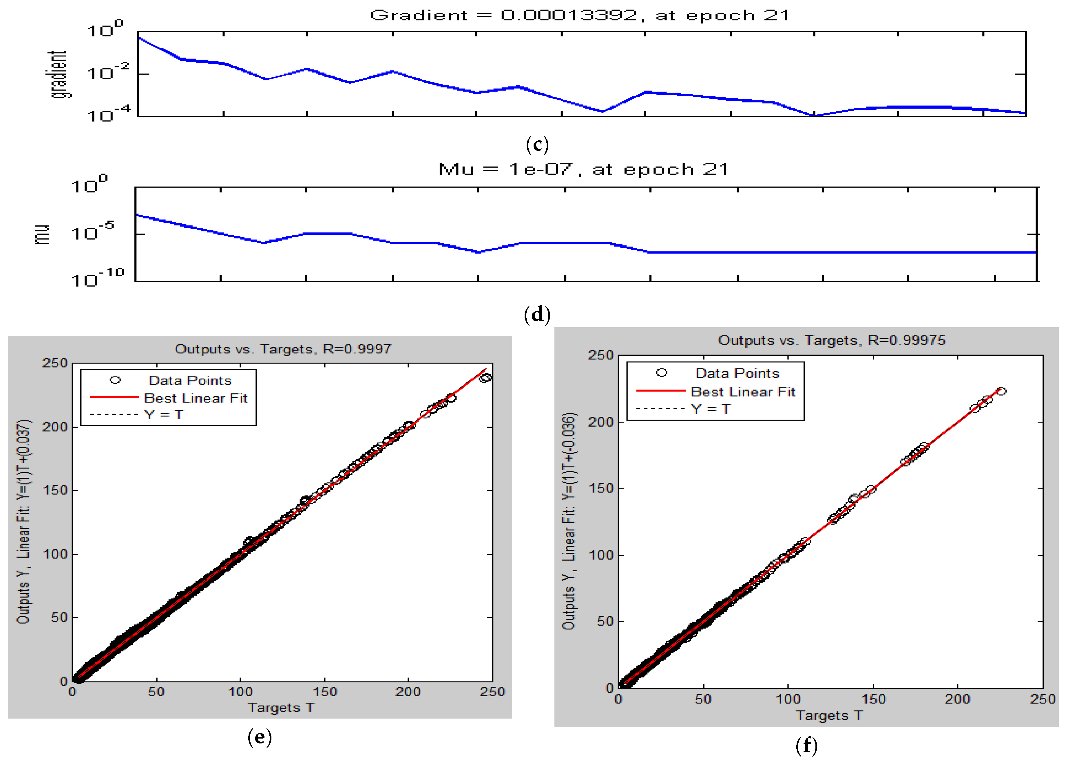
The final decision made for this study was to build two ANN models, using one hidden layer with fifteen hidden nodes. A single parameter in the output layer was used, given that the target value is only the energy consumption per hour of material hauled by the excavator; this represents the first model. For this, 90% of the data (i.e., 4629) were used in the training of the neural network, and the remaining 10% (i.e., 463) of the total data were used for testing the constructed network and to verify the final results. This design of ANN model for energy prediction was selected based on the minimum value of mean square error (0.00000851) produced by this combination (5-15-1) with R-values of 0.99972 and 0.99974 for training and testing output versus target respectively, at a level of learning rate of 0.1 and with 15 iterations to obtain an optimum representation. Similarly, a second ANN model used the prediction of CO2 emissions per hour of material hauled by the excavator as a single output parameter, together with one hidden layer with fifteen hidden nodes. Again, 90% of the data (i.e., 4629) were used in the training of the neural network, and the remaining 10% (i.e., 463) of the total data were used both for testing the constructed network and for verifying the final results. This model was also selected based on the minimum value of mean square error (0.00000895) produced by this combination (5-15-1) with R-values of 0.99970 and 0.99975 for training and testing output versus target respectively, at a level of learning rate of 0.1 and with 21 iterations to achieve an optimum representation. The architectural structure of the optimal ANN models is shown in Figure 4, showing three layers with their connections.
In order to produce an accurate estimation formula based on the ANN model, the data used in the model should first be preprocessed (i.e., through normalizing and scaling) to modify the training environment of the neural network [60,64,65,66]. The input and output data were scaled within the range 0.1 to 0.9 in order to avoid the problem of a slow learning rate at the edges of the data boundaries, and to ensure precision of the output range based on the quality of the sigmoid function in the backward propagation learning algorithms in relation to the default scaled data between 0.0 to 1.0 [60]. The scaling formula for input and output data is shown in Equation (5), which was used here to scale the data within the ranges 0.1 to 0.9 [60].
where Xs represents the normalizing/scaling value of the input data, xi is the value of input data for each parameter (i.e., 1, 2, 3,…, n), xmin is the minimum value of the input data for each parameter, and xmax is the maximum value of the input data for each parameter. In order to develop a prediction formula based on the best result from the ANN model, the values of weight connections and thresholds (i.e., bias) for input to hidden layer and hidden to output layer are essential elements in formulating a final expression for predicting energy consumption and CO2 emissions per hour of excavators. The matrix representation of the prediction formula for both ANN models was preferred because it offers the simplest version for users and practitioners in the field. The following (Section 2.4.1 and Section 2.4.2) describe the matrices for weight connections between the input and hidden layers and the hidden and output layers, input parameters and bias values. In addition, mathematical operations were used on the matrices to produce a final estimation for energy and CO2 emissions per hour of material hauled by an excavator.
2.4.1. Matrix Expressions and Final Formula for Energy Prediction from the Proposed ANN Model
A matrix representation for calculating a final formula for predicting energy consumption per hour of material hauled by excavators was based on the minimum error performances of the proposed ANN model. Consequently, a matrix “A” represents the weight connection matrix between the input and hidden layers (For i = 1, 2,…, n; j = 1, 2,…, m; n = 15 and m = 5), a matrix “B” represents the scaled values for the input parameters (where b = 1, 2,…, q; q = 5) (i.e., element “b1” is digging depth, “b2” cycle time, “b3” bucket payload, “b4” engine horsepower, and “b5” load factor), a matrix “C” represents the bias values (i.e., threshold) of nodes in the hidden layer (where c = 1, 2,…, p; p = 15), a matrix “H” represents the weights connection vector matrix between the hidden and output layers (where h = 1, 2,…, O; O = 15), and “θy” represents the bias value (i.e., threshold) of nodes in the output layer.
where “D” represents the resultant matrix of the multiplication of the weight connections and scaled input parameters matrices, “E” represents a summation matrix for “D” and “C”, “F” represents a matrix resulting from applying a sigmoid function to each weight connection between the input and hidden layers, consisting of fifteen elements (i.e., f1; f2; f3; f4; f5; f6; f7;……..; f15), “K” is a vector matrix for elements facing each other in both the “F” and “H” matrices (note that this step is not typical for matrix multiplication, but it is regarded as multiplication only for parallel elements in both of them), “S” represents the summation values of the bias value of the node output layer and the summation values for the elements of the “K” matrix (For i = 1, 2,…, n; n = 15), and “Ens” represents a prediction value for excavator hourly energy consumption (MJ/h) of material excavated.
2.4.2. Matrix Expressions and Final Formula for CO2 Emission Prediction from the Proposed ANN Model
A matrix representation for calculating the final formula for predicting CO2 emissions per hour of material hauled by excavators is based on the minimum error performances and robust values of the correlation coefficient for the proposed ANN model. Consequently, a matrix “AA” represents the weight connections matrix between the input and hidden layers (For i = 1, 2,…, n; j = 1, 2,…, m; n = 15 and m = 5), a matrix “B” represents scaled values for input parameters (where b = 1, 2,…, q; q = 5) (i.e., element “b1” is digging depth, “b2” cycle time, “b3” bucket payload, “b4” engine horsepower, and “b5” load factor), a matrix “CC” represents the bias values (i.e., threshold) of nodes in the hidden layer (where cc = 1, 2,…, p; p = 15), a matrix “HH” represents the weight connections vector matrix between the hidden and output layers (where h = 1, 2,…, O; O = 15), and “θyy” represents the bias value (i.e., threshold) of nodes in the output layer.
where “DD” represents the resultant matrix of multiplying the weight connections and scaled input parameters matrices, “EE” represents a summation matrix for “DD” and “CC”, “FF” represents the matrix result after applying a sigmoid function to each weight connection between the input and hidden layers, “KK” is a vector matrix for elements facing each other in both “FF” (where FF = [ ff1; ff2; ff3; ff4; ff5; ff6; ff7;……..; ff15]) and “HH” matrices (note that this step is not a typical matrix multiplication, but it is regarded as multiplication only for the parallel elements in both of them) (i = 1, 2,…, n; n = 15), “SS” represents the summation values of the bias value of the node output layer and the summation values for elements of the “KK” matrix, and “Ems” represents a prediction value for excavator CO2 emissions per hour (kg/h) of material excavated.
The matrix size of the weight connections for the prediction equation is mainly dependent on the number of hidden layers, and on having nodes in each hidden layer that have more weight connections, which would produce a complex manual computation. However, reducing the size of the matrices requires the selection of a minimum number of nodes in the hidden layer in order to reduce the size of the weight connection matrix. In addition, the minimum number of hidden layers should be sufficient to achieve an acceptable degree of accuracy and validation. Thus, the adoption of fifteen hidden nodes gives a high degree of accuracy according to the values of mean square error and correlation coefficient, which may give us a large, but not complex, matrix that can be solved using an Excel spreadsheet that is available to, and widely used by, all practitioners in this field. A faster and more advanced method could use Matlab, as used in this study.
2.5. Relative Importance and Sensitivity Analysis of Excavator Input Factor on Energy Consumption and CO2 Emissions
When we need to select the best excavator for earthwork activities, the relative importance of the various input parameters in the designed ANN models is significant for an understanding of the impacts of the parameter on the desired output, and for validation. Understanding the influence of each input parameter on the final output of the proposed ANN model is an essential procedure when comparing different available excavator options and making an optimal choice at an earlier stage of earthwork activities. In addition, identifying and controlling input parameters that exert more effect on the final output of the ANN models (i.e., energy and emission) can help to reduce energy consumption and CO2 emissions associated with the excavators. For instance, if we have two models of excavators that are different in terms of operational characteristics, we can estimate the environmental impact of each of them for each hour of material hauled and, by comparing them with environmental conditions and the productivity performance rate, select the optimum option. In 1991, Garson [67] proposed the partitioning weights method to determine the effects of different input parameters on the outputs, and this method was adopted by [68]. It has been used in this study in order to determine the relative importance of the various input parameters that impact on excavator energy consumption and CO2 emissions per hour for various operational conditions within all operational scenarios that were tested with generated data.
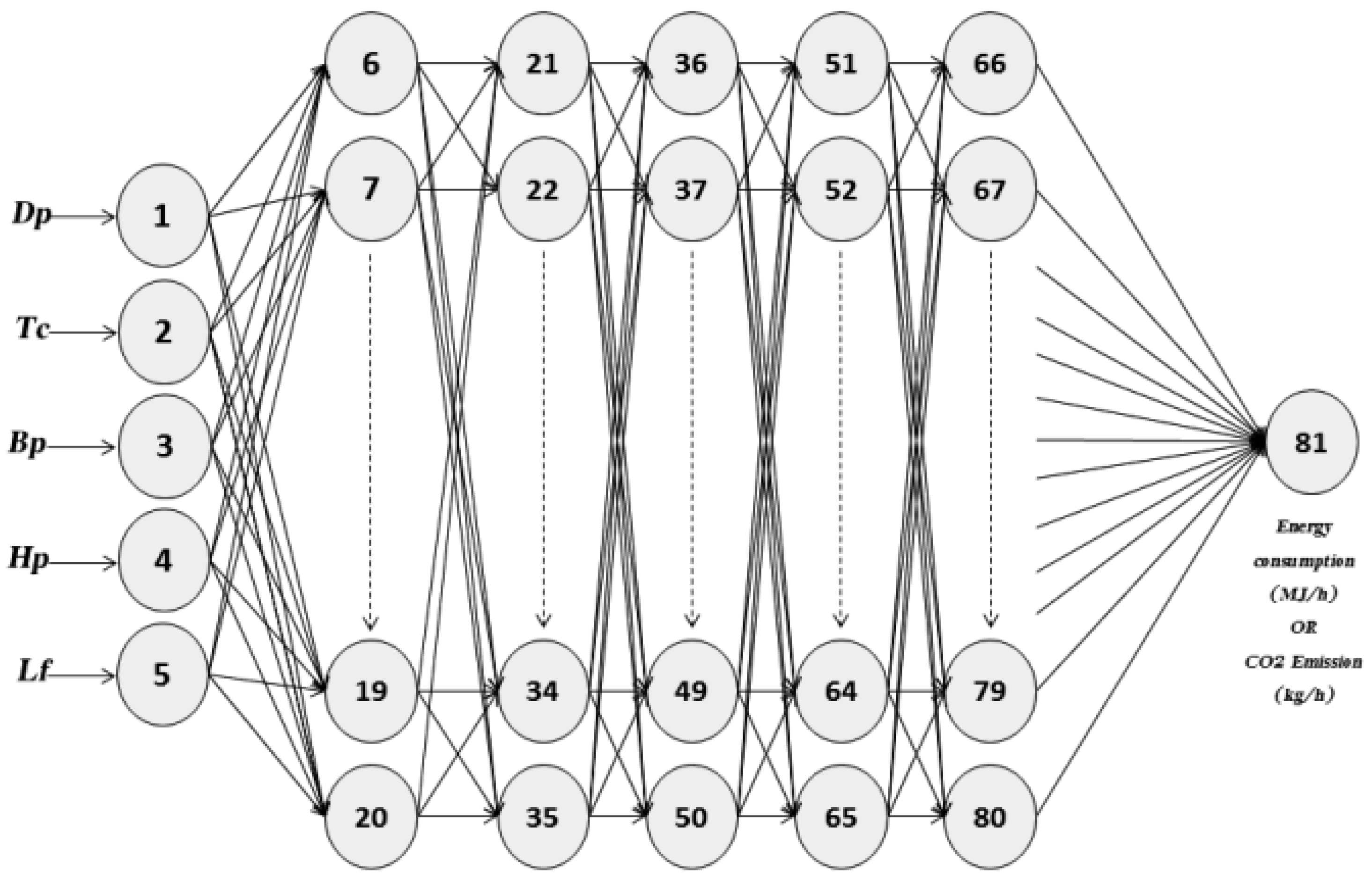
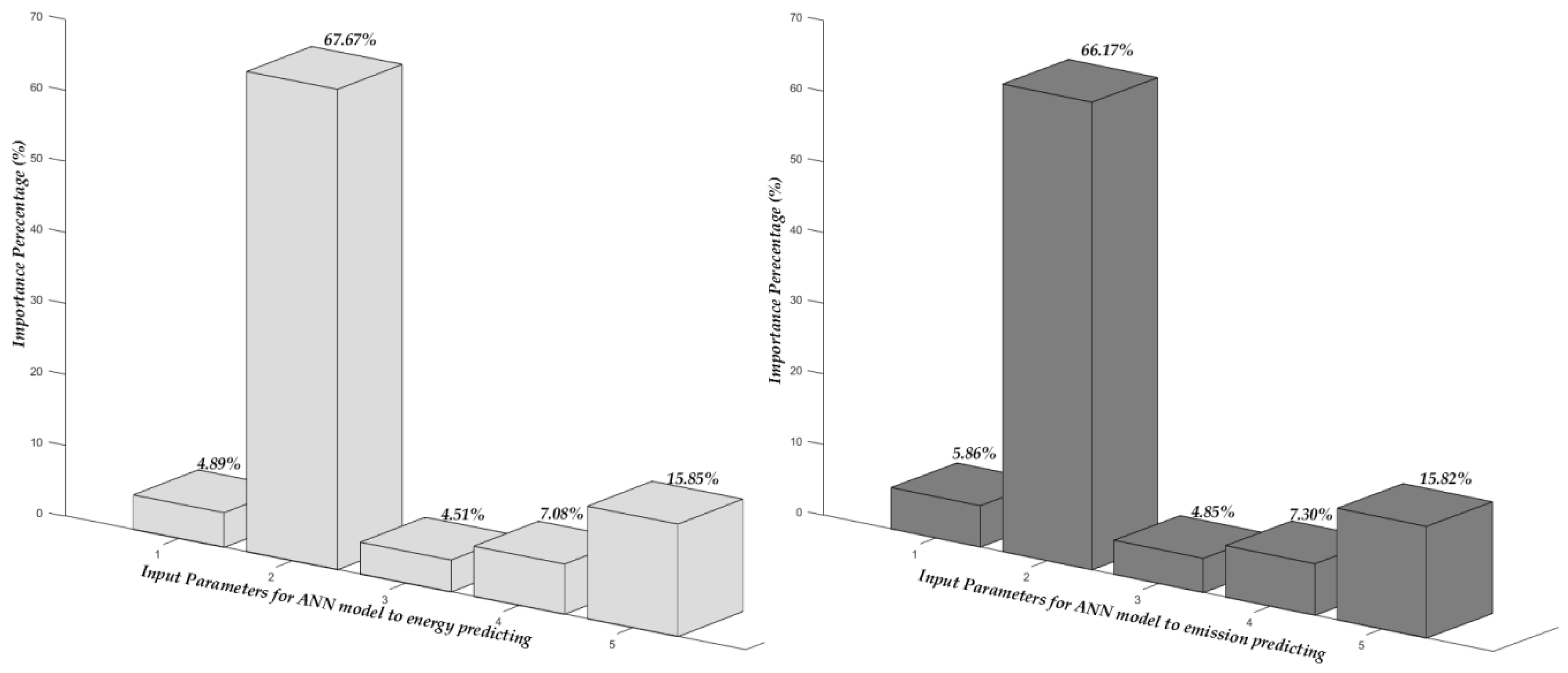
In both of the proposed ANN models, the number of hidden layers was increased to five from the one that was used to build the prediction equations, since more hidden layers filter the data within the neural network more. Each hidden layer has fifteen hidden nodes (see Figure 5), and each node in each layer is fully connected to the nodes pre-layer and post-layer in the ANN model. Using the same percentage of data from the whole database that was used to create the training and testing data subsets, both ANN models were run several times until they achieved the same values for mean square error as the prediction models did. Consequently, the most important parameter influencing energy consumption and CO2 emissions per hour for the excavator in both of the proposed ANN models was found to be the cycle time (Tc), at 67.67% and 66.16% respectively, which involves excavating, swing, loading and returning to the digging start point. Of second highest importance was engine load factor (Lf) (15.85% and 15.82%), followed by horsepower (Hp) (7.08% and 7.30%), digging depth (Dp) (4.98% and 5.86%), and bucket payload (Bp) (4.51% and 4.85%), for both ANN models. This result is shown in Figure 6, where cycle time is a demonetized factor for outputs of both models.
3. Multivariate Linear Regression Formulae for Predicting Energy Consumption and CO2 Emissions Compared with ANN Models
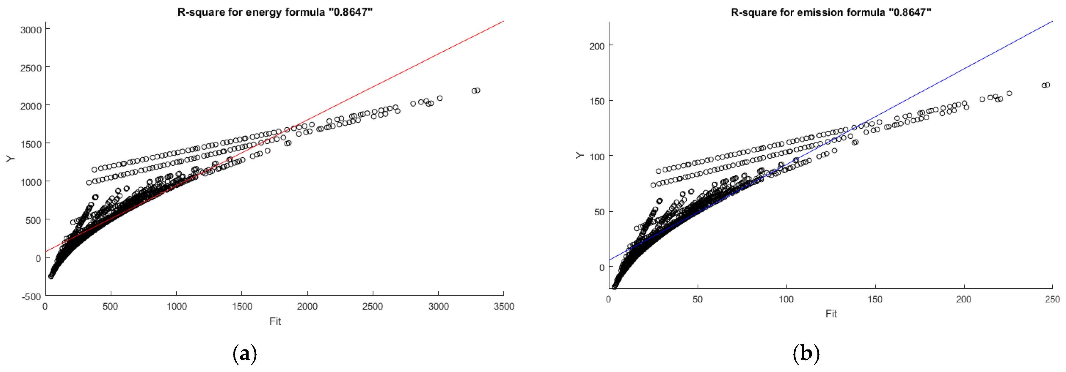
A multivariate linear regression (MLR) analysis technique was applied to the energy and emissions database of the excavators in this study to produce the simplest formulae for predicting both of the target parameters in the ANN models. A regression analysis formula can be considered an easy expression to follow and implement, despite its inadequacy in representing nonlinear behaviors for real-world systems. MLR was used in this study to show the accuracy of the ANN predicting model by comparing the outputs of both models with those from MLR. Furthermore, MLR can be achieved using matrices with Matlab code [67,69], which shows the intercept value “Α” and slopes “ß” (i.e., Beta coefficient) for each input parameter in the final expressions. MLR analysis was implemented on a normal scale database, and this means users would not need to scale input data then remove that scaling from output values. There are two formulae modeled as a MLR function of Dp, Tc, Bp, Hp and Lf for predicting excavator energy consumption and CO2 emissions per hour of material excavated. The analysis results are shown in the following mathematical models (see Equations (18) and (19)). Both the energy and the emissions prediction formulae are based on the value R-square being 0.8647 (see Figure A3a,b).
where “EnR” and “EmR” represent, respectively, hourly energy consumption and CO2 emissions of material hauled by the excavator; “Dp” is digging depth; “Tc” is cycle time; “Bp” is bucket payload; “Hp” is horsepower; and “Lf” is load factor. Intercept value “Α” and slope values “ß” for each formula are shown in Table 3.
4. Results and Discussion
The results of this study focused on the energy consumption and CO2 emissions of excavators, and can be categorized thus: (1) the proposed ANN models for predicting energy consumption and CO2 emissions; (2) identification of factors that have large impacts on the energy consumption and emissions; and (3) comparing the results of a multivariate linear regression formula with ANN model outputs to provide evidence for adopting ANN models as the optimum prediction formulae.
By examining different combinations of hidden node numbers, sizes of training and testing database subsets, with a learning rate of 0.1, the ANN model was designed with fifteen hidden nodes in a single hidden layer, based on the best performance of the neural network after training using a trial-and-error method (see Table A1 and Table A2). In addition, the selection of the number of hidden nodes in this case was also carried out using trial-and-error, from a range of different rule-of-thumb techniques, as suggested by various researchers. Hecht-Nielsen (1990) and Maureen (1991) suggested that the number of hidden nodes in the single hidden layer in the neural network should be equal to double the number of the input parameters plus one (2n + 1) [70,71]. Masters (1993) suggested the number of hidden nodes should be equal to the square root of multiplying the number of outputs and inputs ((n × m)1/2) [72]. Fletcher et al. (1993) stated the number of hidden nodes should be tested with intervals of ((2(n))1/2 + m) to (2n + 1) [73]. Hegazy et al. (1994) suggested the number of hidden nodes should be equal to one half of the total number of input and output parameters (i.e., 1.5 × (n + m)) [74], where n and m represent, respectively, the number of input and output parameters in all expressions given in this section. Although there are no strict rules that should be followed, based on these previous suggestions, the proposed range for the number of hidden nodes in the ANN prediction models should be between 3 and 11 as a guideline for finding the optimum number of hidden nodes. Therefore, the ANN prediction models were tested with different node numbers within the selected intervals, and showed good results with most of these numbers. However, the ANN models also showed a capacity to reduce the mean square error (MSE) for prediction values with an increasing number of hidden nodes. Consequently, the trials were extended to include thirteen and fifteen hidden nodes, with trial-and-error used to pick the optimum number [63]. Therefore, fifteen hidden nodes was seen to be the best design within the tested range of nodes for processing elements in each hidden layer in both of the ANN prediction models. This selection is also supported by the general rule proposed by Jadid et al. 1996, which gives the maximum number of nodes in the hidden layer [75]. Thus, the upper limit in this study is approximately 18 nodes, based on their rule for a range value of 10.
The efficiency of both ANN prediction models was confirmed using the minimum value of MSE for the training performance with the acceptance value of the correlation coefficient (R) [63] as shown in Table A1 and Table A2, and Figure A1a–f and Figure A2a–f. Furthermore, both of the proposed ANN prediction models are considered to be good prediction formulae based on their values of MSE (0.00000851 and 0.00000895) and R (0.99974 and 0.99975), thereby providing guidelines for the selection of the best model to meet the target function [63]. Hence, the ANN models provides an accurate prediction of the energy consumption and also the CO2 emission using the linear relationship between fuel consumption and CO2 proposed by Wojciech G. et al. 1999 [76], and adopted by Yutong G. et al. 2007 [77].
In both of the proposed ANN models, the input data were scaled between 0.1 and 0.9, as mentioned in Section 2.4 and based on Equation (5). This was done in order to reduce the noise from data at the boundaries. Thus, the values produced using the prediction Equations (11) and (17) are the scaled values for energy consumption and CO2 emissions. Consequently, these values should be rescaled using Equation (20) to arrive at the actual prediction values for energy consumption and CO2 emissions per hour.
where Yr represents the value of rescaling output data (i.e., actual prediction values), ys is the normalizing/scaling value of the output (i.e., the value calculated using the prediction Equations (11) and (17)), ymin is the minimum value of the original output data, and ymax is the maximum value of the original output data.
A sensitivity analysis was carried out to identify which of the input parameters had the largest effect on the target output. The relative importance of both the input parameters and the output parameter for both of the proposed ANN models was assessed using MATLAB code, based on the premise that partitioning weights is an acceptable approach for this objective [67,68]. Cycle time is the dominant factor on the output values for all five main input parameters for both of the proposed ANN models. The Caterpillar performance handbook presents excavator specifications and cycle times based on working conditions [78]. However, cycle time is affected by other operational parameters such as bucket size, swing angle, and truck position [79]. In this study, the proposed model uses a cycle time identified from the manufacturer’s handbook using specific swing angle, depth of cut, type of earth, and minimum distance to truck [41,79], for various earth densities with different excavating depths. Therefore, the cycle time for each excavator can be estimated for different operating conditions in the project such as excavating depths and type of earth [80] based on physical quantities [41,78] such as the cutting and loading force required for digging. This allows for the selection of the optimal excavator based on typical engineering project characteristics such as earth type and digging depth [41].
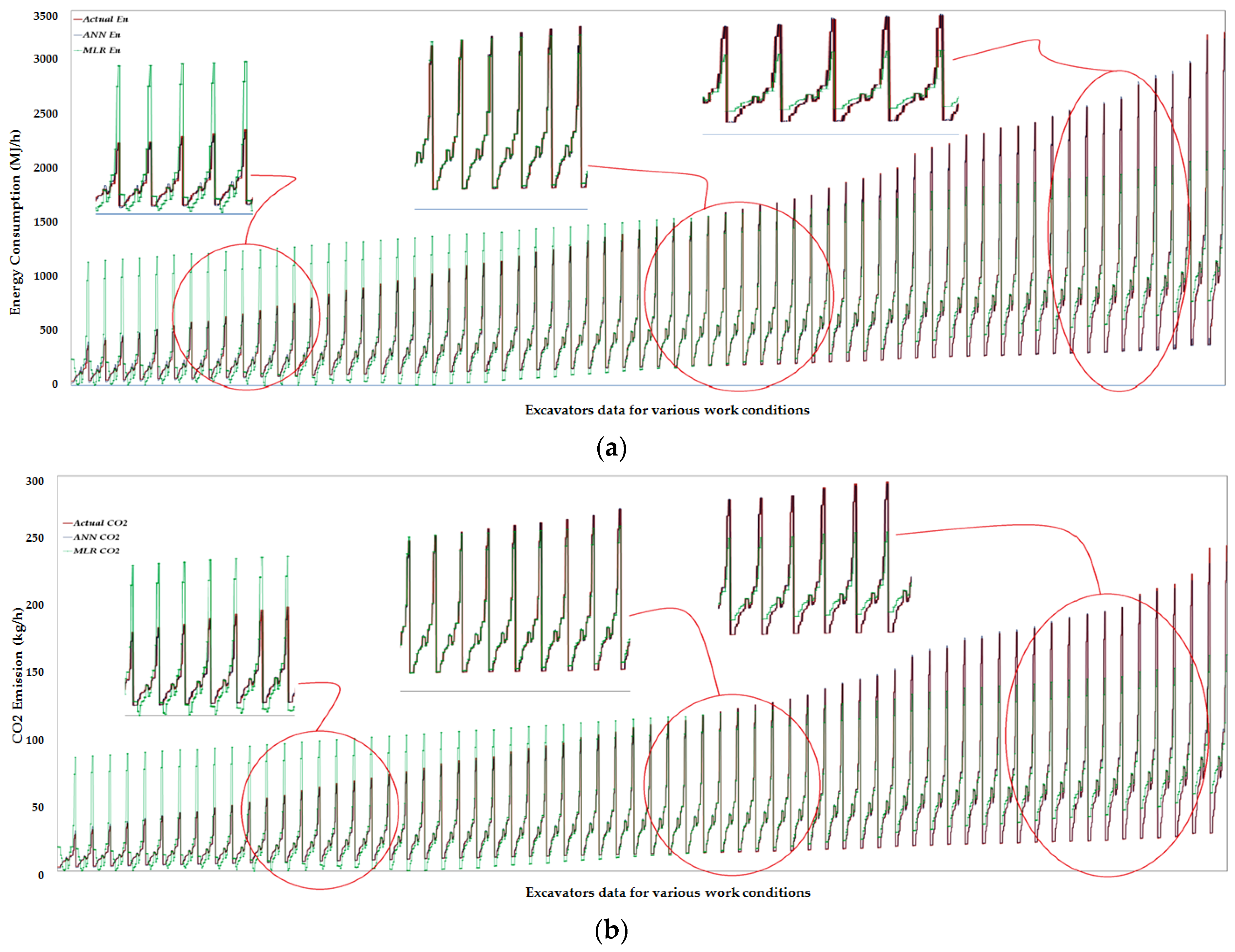
The results of this study can be implemented practically, especially given that the findings of previous research regarding excavator work management have also highlighted that cycle time is an important factor in terms of controlling excavator performance and productivity rates [66,80]. Cycle time is considered a basic metric for loading performance, one that impacts the productivity rates of construction equipment [80,81]. Cycle time for each operation mode is one of the main operational parameters that effect on the level emission of excavators of earthmoving operations [79]. Efficient excavating cycle time is a best idea that leads to fuel saving [82]. Moreover, Komatsu [83] noted the major benefit of reducing cycle time by about 11%, leading to a fuel consumption saving of 23% in excavator operations when adjustment for other factors relevant to fuel consumption, such as engine power, are made. Thus, identifying the major effect of this parameter on the output can be seen as beneficial when controlling and reducing the energy consumption and CO2 emissions of excavators in the earlier stages of construction projects. It allows an ideal plan to be designed which minimizes time lost during excavator operations over each cycle. Figure 7a,b shows the variation in the actual and predicted values (for both ANN and MLR) for energy consumption and CO2 emissions for different excavator models for the various cycle times that work in the different site conditions , showing good agreement between the actual and predicted values for ANN models. It can be seen that the highest values of energy and emissions were produced from each excavator model at the longer cycle time for the same specific conditions and characteristics for each operational scenario. In addition, load factor was considered the second most important factor that impacted on the energy and emission of excavators by Mario et al. (2016) who showed the variation of load factor values in different operational scenarios [43]. However, load factor effects investigated for other heavy duty diesel equipment such as bulldozers have shown that a reduction 15% of load factor may have a significant effect on reducing fuel consumption and emission CO2 [84].
Multivariate linear regression (MLR) analysis was carried out twice on the same generated data for the five input parameters for each output parameter in order to predict energy consumption and CO2 emissions per hour, respectively. Furthermore, regression analysis can be considered as both evidence of, and a method to demonstrate, the validity of specific results of the prediction values from both of the proposed ANN models. The images in Figure 7a,b are constructed to demonstrate the accuracy of the ANN models in comparison with the MLR of various excavators in different work conditions. The x-axis represents the various work situations produces the different cycle-time for different excavators where each excavator operates at a specific cycle time, depth and earth type generating the engine load shown on the y-axis as energy or CO2 emissions. In this case, based on the comparison between the actual values (i.e., the original data used to train both models) for energy and CO2 emission with two predicted values (i.e., ANN and MLR), we can see consistency between the results of the ANN models with actual data for all operational scenarios through the specific ranges, while MLR results show divergent behavior with the actual data for several operational scenarios (see Figure 7a,b). Although these results are acceptable, based on the best value for R-square (0.8647) in both the regression models, it is still a linear model and does not represent an accurate picture of the complex connections between independent parameters. Thereby, this demonstrates the efficiency of the proposed ANN models as prediction formulae for use at an early stage of the construction process in the planning phase when there is a lack of detailed information. The ability of ANN to tackle complex relationships between independent variables that cannot be solved by more traditional methods has been demonstrated by other researches [85,86,87].
In addition, the originality value of this research lies in providing a method to estimate energy consumption and emissions (CO2) in the early planning stages of construction projects despite the practicalities of the shortage of information and details about construction processes during this stage [39]. To overcome this shortfall, the availability of other details from preliminary surveys and investigations on geotechnical information, level/density of cutting layers, and the operational characteristics of the machines available to a construction company or contractor are employed. Furthermore, existing methods to estimate energy use and CO2 emissions might need more detailed information and effort before application or the calculation of certain parameters or details, for instance, productivity rate [35,88], engine speed and other engine operational characteristics [3], in order for those formulas to be applied. The research’s results will thus be of interest to those planning and estimating earthmoving and similar operations in construction projects because it can provide an indication of energy consumption and CO2 emissions before the construction phase commences.
5. Conclusions
For construction management, most studies published have linked artificial neural networks (ANN), an advanced programming technique with a feedforward neural network, with a backpropagation learning algorithm to deal with nonlinear problems. The main aim of this paper was to present models for predicting the energy consumption and CO2 emissions of excavators per hour of material hauled. To do this, data relating to energy consumption have been applied to artificial neural networks in order to model energy consumption and CO2 emissions per hour for excavators. In each prediction model, five input parameters were used with one output parameter, with the ANN model proving that the neural network is capable of modeling and predicting with high accuracy. Moreover, the ANN model has shown the relative importance of the input parameters and their effects on the output. The cycle time of excavators is the dominant factor (≈67%) for levels of energy consumption and CO2 emissions per hour of material hauled by the excavator; the load factor is the second most dominant factor (≈15.9%). Multivariate linear regression (MLR) analysis was carried out to confirm that the results from the ANN prediction models were the best prediction values. The ANN model has displayed an excellent correlation with independent parameters in respect of developing an efficient predictive formula that can compensate for the lack of construction process details when projects are in the early planning stages. The ANN prediction equations, in the form of matrices, are a good aid for planners and practitioners in construction project management when estimating energy consumption and CO2 emissions for each hour of earth-moving in the early (i.e., planning) stage (i.e., limited details) of construction projects, and when selecting the optimum excavator for earth-moving while also considering environmental impacts.
These ANN models can be used to predict energy use and emissions from all types of excavators that fall within the range of the operational characteristics for excavators listed in Table 1 and Table 2. One limitation of this research could be considered the assumption that excavators operate in a steady state and with the same performance efficiency throughout excavation operations. Another limitation could be considered to be that using basic data extracted from the manufacturer’s handbook for the excavators to generate the input data of the proposed models ignores the effects of uncertain conditions such as a long idle time when the excavator has to be moved to a new location, as well output data for energy and CO2 emission depend on indirect measurement. The model presented here will be further extended to use different values of performance efficiencies for excavator fleets in order to cover all real-life operational scenarios where excavators are employed in earth-moving operations. Furthermore, study of other parameters that highly affect behavior under different conditions of earth density and bucket payload such as engine torque to compare the prediction efficiency of the proposed model in the case of use engine load factor or engine torque would be interesting. In addition, the model will be adapted consider other types of greenhouse gas (GHG) emissions and particulate matter.
Author Contributions
The different knowledge and experience of each author has contributed equally to the development and final version of the article. As the main author, Hassanean Jassim wrote and compiled most of this paper. The proposed model and application were also written and carried out by Hassanean Jassim. Weizhuo Lu suggested and reviewed many ideas in the paper to support the work. Thomas Olofsson supervised and reviewed the work throughout the study. Finally, all authors were involved in all steps of this study.
Conflicts of Interest
The authors declare no conflict of interest.
Appendix A
Figure A1.
(a–f) Graphical representation of the properties of the ANN model proposed for energy prediction.
Figure A1.
(a–f) Graphical representation of the properties of the ANN model proposed for energy prediction.

Figure A2.
(a–f). Graphical representation of the properties of the ANN model proposed for emissions prediction.
Figure A2.
(a–f). Graphical representation of the properties of the ANN model proposed for emissions prediction.


Figure A3.
(a,b) Regression representation for energy and emissions prediction formulae.


Table A1.
Trials of different combinations within ANN model to select the optimal energy model performance.
Table A1.
Trials of different combinations within ANN model to select the optimal energy model performance.
| Case | C * | N * | L * | Straining | Stesting | MSE | Epochs | Rtraining | Rtesting |
|---|---|---|---|---|---|---|---|---|---|
| A | 1 | 5-3-1 | 0.1 | 4073 | 1019 | 0.00001974 | 79 | 0.99755 | 0.98361 |
| 2 | 5-3-1 | 0.1 | 4364 | 728 | 0.00007876 | 91 | 0.99715 | 0.99748 | |
| 3 | 5-3-1 | 0.1 | 4526 | 566 | 0.00007665 | 76 | 0.99718 | 0.99743 | |
| 4 | 5-3-1 | 0.1 | 4629 | 463 | 0.00007479 | 71 | 0.99724 | 0.99712 | |
| 5 | 5-3-1 | 0.1 | 4700 | 392 | 0.00026406 | 63 | 0.98964 | 0.98722 | |
| 6 | 5-3-1 | 0.1 | 4752 | 340 | 0.00000995 | 85 | 0.99967 | 0.99968 | |
| B | 7 | 5-6-1 | 0.1 | 4073 | 1019 | 0.00000987 | 71 | 0.99755 | 0.98362 |
| 8 | 5-6-1 | 0.1 | 4364 | 728 | 0.00007876 | 64 | 0.99715 | 0.99748 | |
| 9 | 5-6-1 | 0.1 | 4526 | 566 | 0.00007665 | 81 | 0.99718 | 0.99743 | |
| 10 | 5-6-1 | 0.1 | 4629 | 463 | 0.00029514 | 78 | 0.98904 | 0.99048 | |
| 11 | 5-6-1 | 0.1 | 4700 | 392 | 0.00098040 | 38 | 0.96099 | 0.95960 | |
| 12 | 5-6-1 | 0.1 | 4752 | 340 | 0.00000994 | 11 | 0.99795 | 0.99821 | |
| C | 13 | 5-7-1 | 0.1 | 4073 | 1019 | 0.00001660 | 38 | 0.99755 | 0.98361 |
| 14 | 5-7-1 | 0.1 | 4364 | 728 | 0.00007876 | 42 | 0.99715 | 0.99748 | |
| 15 | 5-7-1 | 0.1 | 4526 | 566 | 0.00007665 | 63 | 0.99718 | 0.99743 | |
| 16 | 5-7-1 | 0.1 | 4629 | 463 | 0.00007479 | 44 | 0.99724 | 0.99712 | |
| 17 | 5-7-1 | 0.1 | 4700 | 392 | 0.00007118 | 73 | 0.99723 | 0.99650 | |
| 18 | 5-7-1 | 0.1 | 4752 | 340 | 0.00001840 | 60 | 0.99053 | 0.98910 | |
| D | 19 | 5-9-1 | 0.1 | 4073 | 1019 | 0.00001970 | 31 | 0.99910 | 0.99034 |
| 20 | 5-9-1 | 0.1 | 4364 | 728 | 0.00002102 | 26 | 0.99924 | 0.99934 | |
| 21 | 5-9-1 | 0.1 | 4526 | 566 | 0.00002886 | 22 | 0.99894 | 0.99887 | |
| 22 | 5-9-1 | 0.1 | 4629 | 463 | 0.00001811 | 28 | 0.99933 | 0.99940 | |
| 23 | 5-9-1 | 0.1 | 4700 | 392 | 0.00002936 | 25 | 0.99885 | 0.99865 | |
| 24 | 5-9-1 | 0.1 | 4752 | 340 | 0.00000976 | 16 | 0.99921 | 0.99921 | |
| E | 25 | 5-11-1 | 0.1 | 4073 | 1019 | 0.00000928 | 27 | 0.99926 | 0.99357 |
| 26 | 5-11-1 | 0.1 | 4364 | 728 | 0.00001489 | 19 | 0.99946 | 0.99954 | |
| 27 | 5-11-1 | 0.1 | 4526 | 566 | 0.00003063 | 14 | 0.99887 | 0.99881 | |
| 28 | 5-11-1 | 0.1 | 4629 | 463 | 0.00001585 | 22 | 0.99942 | 0.99935 | |
| 29 | 5-11-1 | 0.1 | 4700 | 392 | 0.00001616 | 45 | 0.99937 | 0.99933 | |
| 30 | 5-11-1 | 0.1 | 4752 | 340 | 0.00001847 | 34 | 0.99939 | 0.99945 | |
| F | 31 | 5-13-1 | 0.1 | 4073 | 1019 | 0.00001991 | 33 | 0.99879 | 0.99269 |
| 32 | 5-13-1 | 0.1 | 4364 | 728 | 0.00004490 | 67 | 0.99837 | 0.99840 | |
| 33 | 5-13-1 | 0.1 | 4526 | 566 | 0.00001674 | 42 | 0.99938 | 0.99944 | |
| 34 | 5-13-1 | 0.1 | 4629 | 463 | 0.00001441 | 25 | 0.99947 | 0.99951 | |
| 35 | 5-13-1 | 0.1 | 4700 | 392 | 0.00001963 | 42 | 0.99873 | 0.99805 | |
| 36 | 5-13-1 | 0.1 | 4752 | 340 | 0.00000970 | 43 | 0.99897 | 0.99912 | |
| G | 37 | 5-15-1 | 0.1 | 4073 | 1019 | 0.00000999 | 14 | 0.99964 | 0.99967 |
| 38 | 5-15-1 | 0.1 | 4364 | 728 | 0.00000930 | 43 | 0.99969 | 0.99971 | |
| 39 | 5-15-1 | 0.1 | 4526 | 566 | 0.00000925 | 17 | 0.99968 | 0.99969 | |
| 40 | 5-15-1 | 0.1 | 4629 | 463 | 0.00000851 | 15 | 0.99972 | 0.99974 | |
| 41 | 5-15-1 | 0.1 | 4700 | 392 | 0.00000944 | 19 | 0.99962 | 0.99973 | |
| 42 | 5-15-1 | 0.1 | 4752 | 340 | 0.00000937 | 47 | 0.99968 | 0.99968 |
C * = combination number; N * = Design of ANN model; L * = learning rate; Straining = Size of data subset training; Stesting = Size of data subset testing; MSE = Mean square error for best training performance; Epochs = number of iterations required to produce best output; Rtraining = Correlation coefficient for output training data subsets (output vs. target); Rtesting = Correlation coefficient for output testing data subsets (output vs. target).
Table A2.
Trials of different combinations within ANN model to select the optimal emissions model performance.
Table A2.
Trials of different combinations within ANN model to select the optimal emissions model performance.
| Case | C * | N * | L * | Straining | Stesting | MSE | Epochs | Rtraining | Rtesting |
|---|---|---|---|---|---|---|---|---|---|
| A | 1 | 5-3-1 | 0.1 | 4073 | 1019 | 0.00001990 | 41 | 0.99755 | 0.98361 |
| 2 | 5-3-1 | 0.1 | 4364 | 728 | 0.00007876 | 69 | 0.99715 | 0.99748 | |
| 3 | 5-3-1 | 0.1 | 4526 | 566 | 0.00007665 | 66 | 0.99718 | 0.99743 | |
| 4 | 5-3-1 | 0.1 | 4629 | 463 | 0.00007479 | 71 | 0.99724 | 0.99712 | |
| 5 | 5-3-1 | 0.1 | 4700 | 392 | 0.00026406 | 63 | 0.98964 | 0.98722 | |
| 6 | 5-3-1 | 0.1 | 4752 | 340 | 0.00000996 | 84 | 0.99967 | 0.99968 | |
| B | 7 | 5-6-1 | 0.1 | 4073 | 1019 | 0.00008863 | 53 | 0.99755 | 0.98362 |
| 8 | 5-6-1 | 0.1 | 4364 | 728 | 0.00007876 | 64 | 0.99715 | 0.99748 | |
| 9 | 5-6-1 | 0.1 | 4526 | 566 | 0.00007665 | 68 | 0.99718 | 0.99743 | |
| 10 | 5-6-1 | 0.1 | 4629 | 463 | 0.00029514 | 78 | 0.98904 | 0.99048 | |
| 11 | 5-6-1 | 0.1 | 4700 | 392 | 0.00098040 | 38 | 0.96099 | 0.95960 | |
| 12 | 5-6-1 | 0.1 | 4752 | 340 | 0.00002858 | 48 | 0.99795 | 0.99821 | |
| C | 13 | 5-7-1 | 0.1 | 4073 | 1019 | 0.00009781 | 71 | 0.99755 | 0.98361 |
| 14 | 5-7-1 | 0.1 | 4364 | 728 | 0.00007876 | 64 | 0.99715 | 0.99748 | |
| 15 | 5-7-1 | 0.1 | 4526 | 566 | 0.00007665 | 70 | 0.99718 | 0.99743 | |
| 16 | 5-7-1 | 0.1 | 4629 | 463 | 0.00007479 | 74 | 0.99724 | 0.99712 | |
| 17 | 5-7-1 | 0.1 | 4700 | 392 | 0.00007118 | 73 | 0.99723 | 0.99650 | |
| 18 | 5-7-1 | 0.1 | 4752 | 340 | 0.00009549 | 42 | 0.99053 | 0.98910 | |
| D | 19 | 5-9-1 | 0.1 | 4073 | 1019 | 0.00009714 | 49 | 0.99910 | 0.99034 |
| 20 | 5-9-1 | 0.1 | 4364 | 728 | 0.00002102 | 62 | 0.99924 | 0.99934 | |
| 21 | 5-9-1 | 0.1 | 4526 | 566 | 0.00002886 | 22 | 0.99894 | 0.99887 | |
| 22 | 5-9-1 | 0.1 | 4629 | 463 | 0.00001811 | 28 | 0.99933 | 0.99940 | |
| 23 | 5-9-1 | 0.1 | 4700 | 392 | 0.00002936 | 39 | 0.99885 | 0.99865 | |
| 24 | 5-9-1 | 0.1 | 4752 | 340 | 0.00001938 | 69 | 0.99921 | 0.99921 | |
| E | 25 | 5-11-1 | 0.1 | 4073 | 1019 | 0.00000999 | 26 | 0.99926 | 0.99357 |
| 26 | 5-11-1 | 0.1 | 4364 | 728 | 0.00001489 | 37 | 0.99946 | 0.99954 | |
| 27 | 5-11-1 | 0.1 | 4526 | 566 | 0.00003063 | 45 | 0.99887 | 0.99881 | |
| 28 | 5-11-1 | 0.1 | 4629 | 463 | 0.00001585 | 28 | 0.99942 | 0.99935 | |
| 29 | 5-11-1 | 0.1 | 4700 | 392 | 0.00001616 | 41 | 0.99937 | 0.99933 | |
| 30 | 5-11-1 | 0.1 | 4752 | 340 | 0.00000938 | 24 | 0.99939 | 0.99945 | |
| F | 31 | 5-13-1 | 0.1 | 4073 | 1019 | 0.00000963 | 18 | 0.99879 | 0.99269 |
| 32 | 5-13-1 | 0.1 | 4364 | 728 | 0.00001990 | 27 | 0.99837 | 0.99840 | |
| 33 | 5-13-1 | 0.1 | 4526 | 566 | 0.00001674 | 29 | 0.99938 | 0.99944 | |
| 34 | 5-13-1 | 0.1 | 4629 | 463 | 0.00001441 | 25 | 0.99947 | 0.99951 | |
| 35 | 5-13-1 | 0.1 | 4700 | 392 | 0.00003263 | 42 | 0.99873 | 0.99805 | |
| 36 | 5-13-1 | 0.1 | 4752 | 340 | 0.00000923 | 52 | 0.99897 | 0.99912 | |
| G | 37 | 5-15-1 | 0.1 | 4073 | 1019 | 0.00000993 | 28 | 0.99964 | 0.99967 |
| 38 | 5-15-1 | 0.1 | 4364 | 728 | 0.00000930 | 43 | 0.99969 | 0.99971 | |
| 39 | 5-15-1 | 0.1 | 4526 | 566 | 0.00000925 | 17 | 0.99968 | 0.99969 | |
| 40 | 5-15-1 | 0.1 | 4629 | 463 | 0.00000895 | 21 | 0.99970 | 0.99975 | |
| 41 | 5-15-1 | 0.1 | 4700 | 392 | 0.00000944 | 19 | 0.99962 | 0.99973 | |
| 42 | 5-15-1 | 0.1 | 4752 | 340 | 0.00000966 | 23 | 0.99968 | 0.99968 |
C * = combination number; N * = Design of ANN model; L * = learning rate; Straining = Size of data subset training; Stesting = Size of data subset testing; MSE = Mean square error for best training performance; Epochs = number of iterations required to produce best output; Rtraining = Correlation coefficient for output training data subsets (output vs. target); Rtesting = Correlation coefficient for output testing data subsets (output vs. target).
References
- Lewis, P.; Rasdorf, W.; Frey, H.C.; Pang, S.; Kim, K. Requirements and incentives for reducing construction vehicle emissions and comparison of nonroad diesel engine emissions data sources. J. Constr. Eng. Manag. 2009, 135, 341–351. [Google Scholar] [CrossRef]
- Waris, M.; Liew, M.S.; Khamidi, M.F.; Idrus, A. Criteria for the selection of sustainable onsite construction equipment. Int. J. Sustain. Built Environ. 2014, 3, 96–110. [Google Scholar] [CrossRef]
- Heidari, B.; Marr, L.C. Real-time emissions from construction equipment compared with model predictions. J. Air Waste Manag. Assoc. 2015, 65, 115–125. [Google Scholar] [CrossRef] [PubMed]
- Guggemos, A.A.; Horvath, A. Decision-support tool for assessing the environmental effects of constructing commercial buildings. J. Archit. Eng. 2006, 12, 187–195. [Google Scholar] [CrossRef]
- Yi, K. Modelling of on-site energy consumption profile in construction sites and a case study of earth moving. J. Constr. Eng. Proj. Manag. 2013, 3, 10–16. [Google Scholar] [CrossRef]
- Kim, B.; Lee, H.; Park, H.; Kim, H. Greenhouse gas emissions from onsite equipment usage in road construction. J. Constr. Eng. Manag. 2011, 138, 982–990. [Google Scholar] [CrossRef]
- Winther, M.; Nielsen, O. Fuel use and emissions from non-road machinery in Denmark from 1985–2004-and projections from 2005–2030. Environ. Proj. 2006, 1092, 238. [Google Scholar]
- Reinhardt, M.; Kühlen, A.; Haghsheno, S. Developing a pollution measuring system to manage demolition projects complying with legal regulations. In Proceedings of the 2014 (5th) International Conference on Engineering, Project, and Production Management (EPPM), Port Elizabeth, South Africa, 30 November–2 December 2014; p. 116. [Google Scholar]
- Sandanayake, M.; Zhang, G.; Setunge, S.; Thomas, C.M. Environmental emissions of construction equipment usage in pile foundation construction process—A case study. In Proceedings of the 19th International Symposium on Advancement of Construction Management and Real Estate; Shen, L., Ye, K., Mao, C., Eds.; Springer: Berlin/Heidelberg, Germany, 2015; pp. 327–339. [Google Scholar]
- Dallmann, T.; Menon, A. Technology Pathways for Diesel Engines Used in Non-Road Vehicles and Equipment; International Council on Clean Transportation (ICCT): Washington, DC, USA, 2016. [Google Scholar]
- Wong, J.K.; Li, H.; Wang, H.; Huang, T.; Luo, E.; Li, V. Toward low-carbon construction processes: The visualisation of predicted emission via virtual prototyping technology. Autom. Constr. 2013, 33, 72–78. [Google Scholar] [CrossRef]
- Abolhasani, S. Assessment of on-Board Emissions and Energy use of Nonroad Construction Vehicles. Master’s Thesis, North Carolina State University, Raleigh, NC, USA, 2006. [Google Scholar]
- Yang, H.; Xu, Z.; Fan, M.; Gupta, R.; Slimane, R.B.; Bland, A.E.; Wright, I. Progress in carbon dioxide separation and capture: A review. J. Environ. Sci. 2008, 20, 14–27. [Google Scholar] [CrossRef]
- Worrell, E.; Price, L.; Martin, N.; Hendriks, C.; Meida, L.O. Carbon dioxide emissions from the global cement industry. Annu. Rev. Energy Environ. 2001, 26, 303–329. [Google Scholar] [CrossRef]
- Le Quéré, C.; Andrew, R.; Canadell, J.; Sitch, S.; Korsbakken, J.; Peters, G.; Manning, A.; Boden, T.; Tans, P.; Houghton, R. Global carbon budget 2016. Earth Syst. Sci. Data 2016, 8, 605–649. [Google Scholar] [CrossRef]
- Yamasaki, A. An overview of CO2 mitigation options for global warming—Emphasizing CO2 sequestration options. J. Chem. Eng. Jpn. 2003, 36, 361–375. [Google Scholar] [CrossRef]
- Enevoldsen, M.K.; Ryelund, A.V.; Andersen, M.S. Decoupling of industrial energy consumption and CO2-emissions in energy-intensive industries in Scandinavia. Energy Econ. 2007, 29, 665–692. [Google Scholar] [CrossRef]
- The Swedish Transport Administration. The Swedish Transport Administration’s Efforts for Improving Energy Efficiency and for Climate Mitigation; Trafikverket: Karlstad, Sweden, 2012.
- Ainslie, B.; Rideout, G.; Cooper, C.; McKinnon, D. The impact of retrofit exhaust control technologies on emissions from heavy-duty diesel construction equipment. SAE 1999. [Google Scholar] [CrossRef]
- Babbitt, G.R.; Moskwa, J.J. Implementation details and test results for a transient engine dynamometer and hardware in the loop vehicle model. In Proceedings of the 1999 IEEE International Symposium on Computer Aided Control System Design, Kohala Coast, HI, USA, 27 August 1999; pp. 569–574. [Google Scholar]
- Lindgren, M.; Hansson, P. Effects of Transient conditions on exhaust emissions from two non-road diesel engines. Biosyst. Eng. 2004, 87, 57–66. [Google Scholar] [CrossRef]
- Matter, U.; Siegmann, H.; Burtscher, H. Dynamic field measurements of submicron particles from diesel engines. Environ. Sci. Technol. 1999, 33, 1946–1952. [Google Scholar] [CrossRef]
- Yanowitz, J.; McCormick, R.L.; Graboski, M.S. In-use emissions from heavy-duty diesel vehicles. Environ. Sci. Technol. 2000, 34, 729–740. [Google Scholar] [CrossRef]
- Giechaskiel, B.; Riccobono, F.; Vlachos, T.; Mendoza-Villafuerte, P.; Suarez-Bertoa, R.; Fontaras, G.; Bonnel, P.; Weiss, M. Vehicle emission factors of solid nanoparticles in the laboratory and on the road using Portable Emission Measurement Systems (PEMS). Front. Environ. Sci. 2015, 3, 82. [Google Scholar] [CrossRef]
- Frey, H.C.; Rasdorf, W.; Kim, K.; Pang, S.; Lewis, P.; Abolhassani, S. Real-World Duty Cycles and Utilization for Construction Equipment in North Carolina; North Carolina Department of Transportation: Raleigh, NC, USA, 2008.
- Abolhasani, S.; Frey, H.C.; Kim, K.; Rasdorf, W.; Lewis, P.; Pang, S. Real-world in-use activity, fuel use, and emissions for nonroad construction vehicles: A case study for excavators. J. Air Waste Manag. Assoc. 2008, 58, 1033–1046. [Google Scholar] [CrossRef] [PubMed]
- Fu, M.; Ge, Y.; Tan, J.; Zeng, T.; Liang, B. Characteristics of typical non-road machinery emissions in China by using Portable Emission Measurement System. Sci. Total Environ. 2012, 437, 255–261. [Google Scholar] [CrossRef] [PubMed]
- Lewis, P.; Leming, M.; Rasdorf, W. Impact of engine idling on fuel use and CO2 emissions of nonroad diesel construction equipment. J. Manag. Eng. 2011, 28, 31–38. [Google Scholar] [CrossRef]
- Fitriani, H.; Lewis, P. Comparison of predictive modeling methodologies for estimating fuel use and emission rates for wheel loaders. In Proceedings of the 2014 Construction Research Congress: Construction in A Global Network, Atlanta, GA, USA, 19–21 May 2014; pp. 613–622. [Google Scholar]
- Heidari Haratmeh, B. New Framework for Real-Time Measurement, Monitoring, and Benchmarking of Construction Equipment Emissions. Master’s Thesis, Virginia Polytechnic Institute and State University, Blacksburg, VA, USA, 7 May 2014. [Google Scholar]
- Lijewski, P.; Merkisz, J.; Fuc, P.; Kozak, M.; Rymaniak, L. Air pollution by the exhaust emissions from construction machinery under actual operating conditions. Appl. Mech. Mater. 2013, 390, 313–319. [Google Scholar] [CrossRef]
- Hajji, A.M.; Lewis, P. Development of productivity-based estimating tool for energy and air emissions from earthwork construction activities. Smart Sustain. Built Environ. 2013, 2, 84–100. [Google Scholar] [CrossRef]
- Lewis, P.; Rasdorf, W. Fuel use and pollutant emissions taxonomy for heavy duty diesel construction equipment. J. Manag. Eng. 2017, 33, 04016038. [Google Scholar] [CrossRef]
- Hajji, A.M.; Muladi, M.; Larasati, A. ‘ENPROD’ MODEL–estimating the energy impact of the use of heavy duty construction equipment by using productivity rate. In Proceedings of the International Mechanical Engineering and Engineering Education Conferences (IMEEEC), Malang, Indonesia, 7–8 October 2016; AIP Publishing: Melville, NY, USA, 2016; Volume 1778. [Google Scholar]
- Trani, M.L.; Bossi, B.; Gangolells, M.; Casals, M. Predicting fuel energy consumption during earthworks. J. Clean. Prod. 2016, 112, 3798–3809. [Google Scholar] [CrossRef]
- Ofori, G.; Gang, G.; Briffett, C. Implementing environmental management systems in construction: Lessons from quality systems. Build. Environ. 2002, 37, 1397–1407. [Google Scholar] [CrossRef]
- Chen, Z.; Li, H.; Wong, C.T. EnvironalPlanning: Analytic network process model for environmentally conscious construction planning. J. Constr. Eng. Manag. 2005, 131, 92–101. [Google Scholar] [CrossRef]
- Li, H.; Chen, Z. Environmental Management in Construction: A Quantitative Approach; Routledge: Abingdon, UK, 2007. [Google Scholar]
- Braganca, L.; Vieira, S.M.; Andrade, J.B. Early Stage design decisions: The way to achieve sustainable buildings at lower costs. Sci. World J. 2014, 2014, 365364. [Google Scholar] [CrossRef] [PubMed]
- Robichaud, L.B.; Anantatmula, V.S. Greening project management practices for sustainable construction. J. Manag. Eng. 2010, 27, 48–57. [Google Scholar] [CrossRef]
- Caterpillar. Caterpillar Performance Handbook, 42th ed.; Caterpillar Inc.: Peoria, IL, USA, 2012. [Google Scholar]
- Filas, F.J. Excavation, loading, and material transport. In SME Mining Reference Hand Book; Lowrie, R.L., Ed.; Society for Mining, Metallurgy and Exploration: Littleton, CO, USA, 2002; pp. 215–241. [Google Scholar]
- Klanfar, M.; Korman, T.; Kujundžić, T. Fuel consumption and engine load factors of equipment in quarrying of crushed stone. Tech. Gaz. 2016, 23, 163–169. [Google Scholar]
- Lee, T. Military Technologies of the World [2 Volumes]; ABC-CLIO: Santa Barbara, CA, USA, 2008. [Google Scholar]
- Environmental Protection Agency (EPA). Median Life, Annual Activity, and Load Factor Values for Nonroad Engine Emissions Modeling; National Service Center for Environmental Publications (NSCEP): College Park, MD, USA, 2010.
- Clement, S.; Evans, N.; ICLEI-Local Governments for Sustainability. Clean Fleets guide. In Procuring Clean and Efficient Road Vehicles; International Council for Local Environmental Initiatives (ICLEI-Europe) Local Governments for Sustainability: Freiburg, Germany, 2014. [Google Scholar]
- Tyson, K.S.; McCormick, R.L. Biodiesel Handling and Use Guidelines; National Renewable Energy Laboratory: Golden, CO, USA, 2006. [Google Scholar]
- Peterson, C.; Auld, D.; Korus, R. Winter rape oil fuel for diesel engines: Recovery and utilization. J. Am. Oil Chem. Soc. 1983, 60, 1579–1587. [Google Scholar] [CrossRef]
- Bridgwater, A.V. Renewable fuels and chemicals by thermal processing of biomass. Chem. Eng. J. 2003, 91, 87–102. [Google Scholar] [CrossRef]
- Qi, D.; Leick, M.; Liu, Y.; Chia-fon, F.L. Effect of EGR and injection timing on combustion and emission characteristics of split injection strategy DI-diesel engine fueled with biodiesel. Fuel 2011, 90, 1884–1891. [Google Scholar] [CrossRef]
- Zhang, S.; Wu, Y.; Liu, H.; Huang, R.; Yang, L.; Li, Z.; Fu, L.; Hao, J. Real-world fuel consumption and CO2 emissions of urban public buses in Beijing. Appl. Energy 2014, 113, 1645–1655. [Google Scholar] [CrossRef]
- Yoon, S.H.; Park, S.H.; Lee, C.S. Experimental investigation on the fuel properties of biodiesel and its blends at various temperatures. Energy Fuels 2007, 22, 652–656. [Google Scholar] [CrossRef]
- Department of Energy and Climate Change (DECC); Department for Environment, Food and Rural Affairs (Defra). Guidelines to Defra/DECC’s GHG Conversion Factors for Company Reporting; Department for Environment, Food and Rural Affairs: London, UK, 2011.
- Burgess, J.W. Material properties. In SME Mining Reference Hand Book; Lowrie, R.L., Ed.; Society for Mining, Metallurgy and Exploration: Littleton, CO, USA, 2002; pp. 9–11. [Google Scholar]
- Scesi, L.; Papini, M. Geologia Applicata. Vol. 1: Il Rilevamento Geologico-Tecnico; Città Studi: Milan, Italy, 2006. [Google Scholar]
- Gottfried, A. Ergotecnica Edile; Hoepli: Milan, Italy, 2013. [Google Scholar]
- Cross, S.S.; Harrison, R.F.; Kennedy, R.L. Introduction to neural networks. Lancet 1995, 346, 1075–1079. [Google Scholar] [CrossRef]
- Demuth, H.; Beale, M. Neural Network Toolbox; The MathWorks, Inc.: Natick, MA, USA, 1992. [Google Scholar]
- Zhang, G.; Patuwo, B.E.; Hu, M.Y. Forecasting with artificial neural networks: The state of the art. Int. J. Forecast. 1998, 14, 35–62. [Google Scholar] [CrossRef]
- Oreta, A.W.C. Simulating size effect on shear strength of RC beams without stirrups using neural networks. Eng. Struct. 2004, 26, 681–691. [Google Scholar] [CrossRef]
- Upadhyaya, B.R.; Eryurek, E. Application of neural networks for sensor validation and plant monitoring. Nucl. Technol. 1992, 97, 170–176. [Google Scholar]
- Siami-Irdemoosa, E.; Dindarloo, S.R. Prediction of fuel consumption of mining dump trucks: A neural networks approach. Appl. Energy 2015, 151, 77–84. [Google Scholar] [CrossRef]
- Šibalija, T.V.; Majstorović, V.D. Advanced Multiresponse Process. Optimisation; Springer: Berlin, Germany, 2016. [Google Scholar]
- Gulcicek, U.; Ozkan, O.; Gunduz, M.; Demir, I.H. Cost assessment of construction projects through neural networks. Can. J. Civ. Eng. 2013, 40, 574–579. [Google Scholar] [CrossRef]
- Ok, S.C.; Sinha, S.K. Construction equipment productivity estimation using artificial neural network Model. Constr. Manag. Econ. 2006, 24, 1029–1044. [Google Scholar] [CrossRef]
- Tam, C.; Tong, T.K.; Tse, S.L. Artificial neural networks model for predicting excavator productivity. Eng. Constr. Arch. Manag. 2002, 9, 446–452. [Google Scholar] [CrossRef]
- Garson, D.G. Interpreting neural network connection weights. AI Expert 1991, 6, 47–51. [Google Scholar]
- Goh, A. Back-propagation neural networks for modeling complex systems. Artif. Intell. Eng. 1995, 9, 143–151. [Google Scholar] [CrossRef]
- Brown, S.H. Multiple linear regression analysis: A matrix approach with MATLAB. Ala. J. Math. 2009, 34, 1–3. [Google Scholar]
- Hecht-Nielsen, R. Neurocomputing; Addison-Wesley: Boston, MA, USA, 1990. [Google Scholar]
- Caudill, M. Neural network training tips and techniques. AI Expert 1991, 6, 56–61. [Google Scholar]
- Masters, T. Practical Neural Network Recipes in C++; Morgan Kaufmann: Burlington, MA, USA, 1993. [Google Scholar]
- Fletcher, D.; Goss, E. Forecasting with neural networks: An application using bankruptcy data. Inf. Manag. 1993, 24, 159–167. [Google Scholar] [CrossRef]
- Hegazy, T.; Fazio, P.; Moselhi, O. Developing practical neural network applications using back-propagation. Compu. Aided Civil Infrastruct. Eng. 1994, 9, 145–159. [Google Scholar] [CrossRef]
- Jadid, M.N.; Fairbairn, D.R. Neural-network applications in predicting moment-curvature parameters from experimental data. Eng. Appl. Artif. Intell. 1996, 9, 309–319. [Google Scholar] [CrossRef]
- Gis, W.; Bielaczyc, P. Emission of CO2 and fuel consumption for automotive vehicles. Emiss. Tech. Meas. Test. 1999. [Google Scholar] [CrossRef]
- Gao, Y.; Checkel, M.D. Experimental measurement of on-road CO2 emission and fuel consumption functions. Trans. J. Eng. 2007. [Google Scholar] [CrossRef]
- Robert, I.; Peurifoy, P.; Clifford, J.; Schexnayder, P.; Shapira, A. Construction Planning, Equipment and Methods; McGrow-Hill Higher Education: Boston, MA, USA, 2006. [Google Scholar]
- Barati, K.; Shen, X. Emissions modelling of earthmoving equipment. In Proceedings of the International Symposium on Automation and Robotics in Construction, Auburn, AL, USA, 18–21 July 2016. [Google Scholar]
- Ng, F.; Harding, J.A.; Glass, J. An eco-approach to optimise efficiency and productivity of a hydraulic excavator. J. Clean. Prod. 2016, 112, 3966–3976. [Google Scholar] [CrossRef] [Green Version]
- Hall, A.S. Characterizing the Operation of a Large Hydraulic Excavator. Master’s Thesis, University of Queensland, Brisbane, Australia, 28 January 2003. [Google Scholar]
- Fuel Economy. Fuelling Savings in Tough Times; Blutip Power Technologies: Mississauga, ON, Canada, 2015; pp. 38–46.
- Komatsu (Ed.) Komatsu Specification and Application Handbook, 30th ed.; Komatsu Limited: Tokyo, Japan, 2009. [Google Scholar]
- Kecojevic, V.; Komljenovic, D. Impact of bulldozer’s engine load factor on fuel consumption, CO2 emission and cost. Am. J. Environ. Sci. 2011, 7, 125. [Google Scholar] [CrossRef]
- Shavlik, J.W.; Mooney, R.J.; Towell, G.G. Symbolic and neural learning algorithms: An experimental comparison. Mach. Learn. 1991, 6, 111–143. [Google Scholar] [CrossRef]
- Setiono, R.; Leow, W.K.; Zurada, J.M. Extraction of rules from artificial neural networks for nonlinear regression. IEEE Trans. Neural Netw. 2002, 13, 564–577. [Google Scholar] [CrossRef] [PubMed]
- James, C.D.; Davis, R.; Meyer, M.; Turner, A.; Turner, S.; Withers, G.; Kam, L.; Banker, G.; Craighead, H.; Issacson, M. Aligned microcontact printing of micrometer-scale poly-l-lysine structures for controlled growth of cultured neurons on planar microelectrode arrays. IEEE Trans. Biomed. Eng. 2000, 47, 17–21. [Google Scholar] [CrossRef] [PubMed]
- Hajji, A.M.; Lewis, P. Development of productivity-based estimating tool for fuel use and emissions from earthwork construction activities. KICEM J. Constr. Eng. Proj. Manag. 2013, 3, 58–65. [Google Scholar] [CrossRef]
Figure 1.
A framework for the main process used to create an estimation formula.

Figure 2.
Flowchart for generating the training data sets of energy consumption and CO2 emission.

Figure 3.
IDEFO for research framework.

Figure 4.
Architectural structure for the optimal ANN model to predict energy consumption or CO2 emissions.
Figure 4.
Architectural structure for the optimal ANN model to predict energy consumption or CO2 emissions.

Figure 5.
Architectural structure to identify the relative importance of input parameters to the energy consumption or CO2 emission ANN models.
Figure 5.
Architectural structure to identify the relative importance of input parameters to the energy consumption or CO2 emission ANN models.

Figure 6.
Relative importance of input parameters to the energy consumption and CO2 emission ANN models.
Figure 6.
Relative importance of input parameters to the energy consumption and CO2 emission ANN models.

Figure 7.
(a,b) Actual and predicted behavior of energy consumption and emissions for excavators with various operating conditions.
Figure 7.
(a,b) Actual and predicted behavior of energy consumption and emissions for excavators with various operating conditions.

Table 1.
Suitable types of earth excavation and range density for different excavators.
| Caterpillar Excavator Model | Suitable Type of Earth | Bank Density (kg/m3) |
|---|---|---|
| 307C, 308D CR, 308D CR SB, 311D LRR, 312D, 312D L, 315D L, 319D L, 319D LN | Decomposed Rock-Packed Earth | 960–2260 |
| M313D, M315D, M316D, M318D, M322D | Sand/Gravel | 1370–2082 |
| 320D, 320D RR, 321D CR, 323D, 324D, 328D LCR, 329D, 336D, 345D, 365C L and 385C | Hard Clay | 1089–2415 |
Table 2.
Boundary conditions for database generation for different excavator models.
| Excavator Model | Dp (m) | Tc (min) | Bs (m3) | Bf (%) | Hp (kW) | Lf (%) |
|---|---|---|---|---|---|---|
| 307C, 308D CR, 308D CR SB, 311D LRR, 312D, 312D L, 315D L, 319D L, 319D LN | 1.5–3.0 | 0.22–0.28 | 0.37–1.05 | 0.8–1.1 | 41–93 | 0.15–0.91 |
| M313D, M315D, M316D, M318D, M322D | 2.0–4.0 | 0.17–0.23 | 0.8–1.37 | 0.9–1.0 | 95–123 | 0.15–0.91 |
| 320D, 320D RR, 321D CR, 323D, 324D, 328D LCR, 329D, 336D, 345D, 365C L and 385C | 2.3–5.6 | 0.23–0.35 | 1.05–5.0 | 0.65–0.95 | 103–355 | 0.15–0.91 |
Table 3.
The intercept and slope values for regression equations.
| Items | A | ß1 | ß2 | ß3 | ß4 | ß5 | |
|---|---|---|---|---|---|---|---|
| EnR | n | −562.921 | −5.79 × 10⁻⁹ | 8.14 × 10⁻⁹ | 3.25 × 10⁻¹⁰ | 4.45274 | 1177.95 |
| EmR | m | −42.1721 | 1.51 × 10⁻¹⁰ | 3.16 × 10⁻⁹ | 6.31 × 10⁻¹⁰ | 0.33359 | 88.2478 |
© 2017 by the authors. Licensee MDPI, Basel, Switzerland. This article is an open access article distributed under the terms and conditions of the Creative Commons Attribution (CC BY) license (http://creativecommons.org/licenses/by/4.0/).
Share and Cite
MDPI and ACS Style
Jassim, H.S.H.; Lu, W.; Olofsson, T. Predicting Energy Consumption and CO2 Emissions of Excavators in Earthwork Operations: An Artificial Neural Network Model. Sustainability 2017, 9, 1257. https://doi.org/10.3390/su9071257
AMA Style
Jassim HSH, Lu W, Olofsson T. Predicting Energy Consumption and CO2 Emissions of Excavators in Earthwork Operations: An Artificial Neural Network Model. Sustainability. 2017; 9(7):1257. https://doi.org/10.3390/su9071257
Chicago/Turabian StyleJassim, Hassanean S. H., Weizhuo Lu, and Thomas Olofsson. 2017. "Predicting Energy Consumption and CO2 Emissions of Excavators in Earthwork Operations: An Artificial Neural Network Model" Sustainability 9, no. 7: 1257. https://doi.org/10.3390/su9071257
Note that from the first issue of 2016, this journal uses article numbers instead of page numbers. See further details here.