Life Cycle Impact Assessment in the Arctic: Challenges and Research Needs

1
Industrial Ecology Programme and Department of Energy and Process Engineering, Norwegian University of Science and Technology, 7491 Trondheim, Norway
2
Faculty of Biosciences, Fisheries and Economics, The Arctic University of Norway, 9037 Tromsø, Norway
*
Author to whom correspondence should be addressed.
Sustainability 2017, 9(9), 1605; https://doi.org/10.3390/su9091605
Submission received: 17 August 2017
/
Revised: 3 September 2017
/
Accepted: 7 September 2017
/
Published: 8 September 2017
(This article belongs to the Section Sustainable Engineering and Science)
Abstract
:Life cycle assessment (LCA) is increasingly used for environmental assessment of products and production processes to support environmental decision-making both worldwide and in the Arctic. However, there are several weaknesses in the impact assessment methodology in LCA, e.g., related to uncertainties of impact assessment results, absence of spatial differentiation in characterization modeling, and gaps in the coverage of impact pathways of different “archetypal” environments. Searching for a new resource base and areas for operation, marine and marine-based industries are continuously moving north, which underlines the need for better life cycle impact assessment in the Arctic, particularly to aid in industrial environmental management systems and stakeholder communications. This paper aims to investigate gaps and challenges in the application of the currently available impact assessment methods in the Arctic context. A simplified Arctic mining LCA case study was carried out to demonstrate the relevance of Arctic emissions at the midpoint and endpoint levels, as well as possible influences of the Arctic context on the impact assessment results. Results of this study showed that significant research gaps remain in Arctic-dependent life cycle impact assessment, particularly on: (i) the possible influences of the Arctic-specific features on characterization factors for impact assessment (such as seasonality, cold climate, precipitation, and marine dependence); and (ii) the coverage of impact pathways, especially on the under-addressed marine impacts and marine/near-shore dispersion processes. Addressing those identified research gaps and demand for future Arctic life cycle impact assessment could increase the credibility of LCA as an environmental decision-making support tool for Arctic industries and better support sustainable Arctic development.
1. Introduction
Sustainable development in the Arctic has attracted growing attention within the North Polar Region and beyond, largely owing to environmental challenges and emerging human interventions. The Arctic is facing the rapidly occurring environmental changes, especially on climate change and environmental pollution. Since the 1950s, the Arctic region has experienced the greatest regional warming on earth, with an average annual temperature increase by 2–3 °C and in winter by up to 4 °C [1]. Global warming has resulted in shrinking Arctic sea ice and the opening of the Arctic Ocean. In September 2012, the summer sea ice area had shrunk by 55%, compared to the minimum coverage of 7.5 million square kilometers in September 1980 [2]. Moreover, the Arctic is a “sink” for certain pollutants transported from distant sources, such as heavy metals (notably mercury), persistent organic pollutants, radioactivity, and chemicals of emerging concern [3]. For example, Arctic haze, occurring in winter and spring, is due to high concentrations of air pollutants transported to the Arctic, composing of a mixture of sulfate and particulate organic matter and, to a lesser extent, ammonium, nitrate, dust, and black carbon [4]. Because of low temperatures and low biological activity, pollutants in the Arctic tend to persist for long periods of time in the environment and pose health risks to local ecosystems and humans [3]. The expected increase in Arctic industrial activities, such as Arctic shipping and exploration of resources, could potentially cause negative impacts on the local environment, which needs to be assessed in a prospective manner. The Arctic region has huge oil and gas reserves and large mineral reserves, and Arctic seas contain some of the world’s richest commercial fishing grounds [1]. The United States Geological Survey has concluded that about 30% of the world’s undiscovered gas and 13% of the world’s undiscovered oil may be found in the Arctic [5]. In recent year, there is a clear trend on the upsurge in mining activities in most Euro-Arctic regions [6]. Similarly, exploitation of the off shore oil reserves, e.g., along Western Greenland, is expected in the near future [7]. Besides the long-range transport of pollutants, local pollutants from industrial activities in the Arctic could lead to increased pollutant concentrations in the environment and bioaccumulation in food chains. In support of sustainable Arctic development, it is crucial to understand the impacts of local emissions from emerging industrial activities on the Arctic environment in a holistic and proactive way to avoid the late-recognition syndrome of environmental problems. Life Cycle Assessment (LCA) is the most mature life cycle-based method to aid in addressing problems related to environmental sustainability [8]. As an ISO-standardized environmental assessment method, LCA provides a way to systematically evaluate the significance of potential environmental impacts associated with products and production processes, and to support pollution prevention in particular [9]. A major strongpoint of LCA is a life cycle scope and broad inclusion of environmental impacts, including those global impacts caused by spatially distributed contributors such as greenhouse gas emissions and resource extraction. LCA is now a widely used environmental systems analysis tool in industry, academia and government. The European Commission Joint Research Centre (JRC) published the International Life Cycle Data System (ILCD) Handbook in 2010, representing a further confirmation of the importance of LCA as an environmental decision-supporting tool for product development and EU policy making [8]. However, gaps and challenges remain in both life cycle inventory modeling (such as allocating environmental burdens and identifying data uncertainty) and life cycle impact assessment in practice [10]. The current impact assessment models are still in their infancy, especially in the development of some important water- and land-related impact categories, incorporating spatial and temporal differentiation, and addressing ecosystem services [11] and marine ecological impacts [12].
Life cycle impact assessment (LCIA) aims to assess the potential environmental impacts associated with an inventory of environmental emissions and energy and material inputs, which is a crucial step in every LCA study. It was not until the mid-1990s that the interpretation of environmental intervention in LCA started addressing impact assessment. Since the early development of LCIA, the absence of spatially differentiated characterization has been under debate [13,14]. The traditional site-generic characterization factors are based on modeling the fate of substances from emissions in the receiving environment with exclusion of spatial characteristics. However, site-genetic characterization modeling in LCIA sometimes leads to obviously erroneous results [15], which may significantly influence the credibility of LCA and its application to sustainability.
There are two main trends in the recent development of LCIA methods. The first trend concerns consensus building in models and approaches, led by the UNEP SETAC Life Cycle Initiative [16] and the European Platform for LCA [17]. Efforts of this trend are on the development of mutual models for the dispersion of pollutants in the environment [18], definition of human uptake pathways [19], endpoint metrics for human health damage [20], and so on. The second trend focuses on increasing regionalization and the spatial resolution in impact assessment models, since ecosystem characteristics and population densities vary greatly between world regions and countries. Spatially differentiated LCIA methods have been developed since the pioneer work on site-dependent LCIA of acidification in the late 1990s [21]. Two distinct approaches to regionalization in LCA can be defined: (i) using recipient archetypes, e.g., indoor/outdoor, urban/rural, and remote area classification for human recipients [18,22], and soil types for metal fate and availability [23]; or (ii) using specific location by means of GIS or continental/national boundaries [24], national ecozones [25], or regions [26], while the relevant resolution may vary between impact categories [27].
Thus far, spatial differentiation life cycle impact assessment for the Arctic is still very limited, although LCA has been widely used for environmental assessment at continent, region and country levels. In a recent attempt to bridge Arctic environmental science and LCA, Johnsen [28] highlighted the importance of ecotoxicity, acidification, and soot/black carbon in Arctic LCAs, based on survey results from Arctic environmental scientists. To the authors’ knowledge, no LCA is available in the literature focusing on the applicability of the currently available LCIA methods to the Arctic context and on what Arctic-specific features to be included in characterization modeling for future Arctic LCAs.
This paper presents the results of our pre-study with the ultimate aim of developing site-dependent life cycle impact assessment in the Arctic. Firstly, the basic features of the Arctic were summarized, with respect to the environment, biology, and population. Secondly, characterization models and assumptions of the current ready-to-use LCIA methods were revisited, serving as a basis for identifying gaps and challenges in the application of LCA for the Arctic. Thirdly, a simplified LCA case study of a copper ore mine in northern Norway was carried out to demonstrate the relevance of Arctic emissions to both midpoint impacts and endpoint damages. Finally, the possible influence of the Arctic-specific features on the current LCA characterization modeling was discussed and research needs for future Arctic LCAs were suggested.
2. Characteristics of the Arctic Region
2.1. Environment
A common definition of the Arctic is the area north of the Arctic Circle (66°32′ N), approximately outlining the southern boundary of the midnight sun. Alternative definitions are based on temperature (the area north of the 10 °C July isotherm), vegetation or oceanographic characteristics, while Arctic Monitoring and Assessment Programme (AMAP) applies a geographical compromise (Figure 1) delimited by the treeline (trees not growing beyond the northern limit) [29].
The Arctic climate is characterized by “severity, seasonality, and unpredicted variability” [30]. The Arctic-specific physical and geographical properties [29,31] are: (i) extreme seasonality and variation in temperature and precipitation, both intra- and inter-annually; (ii) a strong latitude solar and UV radiation gradient; and (iii) low precipitation, mostly in the form of snow. The annual precipitation is generally less than 500 mm and typically within 200–400 mm, with higher values observed in coastline while lower in the Polar Basin and inlands (inlands proportionally declining with distance from the coast) [29]. Besides Arctic haze, natural fog is typical in the Arctic and more than 100 days per year were recorded in some sites [32]. Low temperatures lead to extensive ice cover of both marine and freshwater, resulting in a high albedo over the year [31].
With only 1% of global ocean volume, the Arctic ocean receives over 10% of global river discharge, which affects salinity and estuaries [33]. The spring melt may carry 80–90% of the annual total runoff over a period of two or three weeks [29]. Field measurements in large rivers of Russian Arctic and North American Arctic show lower shares for the spring flux, but carrying one to two thirds of annual nitrate and dissolved organic carbon (DOC) fluxes over the course of two intensive months (May–June) [33]. Warmer run-off leads to stratification in the receiving freshwater [31] and marine water bodies [34]. In a recent synthesis of Arctic terrestrial hydrology, Bring et al. [35] reviewed the processes, function and change of the central freshwater processes across seven hydro-physiographical regions, as well as effects of hydrological change.
In terms of future trends in the Arctic, winter rainfall and melting events are projected to become more frequent, and to a large extent replace the regular snowmelt in sub-Arctic Norway [36]. According to the 2017 SWIPA (Snow, Water, Ice and Permafrost in the Arctic) assessment coordinated by AMAP, the Arctic Ocean could be largely ice-free in summer as early as the late 2030s, and an intensified Arctic water cycle would increase freshwater flows among land, atmosphere, and ocean [37].
2.2. Biology
While low nutrient availability, cold temperatures and a short growth season lead to a low Arctic productivity inland [29] as well as in the overall marine environment [38], seasonal marine productivity in certain locations is among the highest globally [39]. One adaptation to the Arctic seasonality is high intake when food is available, followed by storage for the following year. Migratory behavior is another, as seen in fish, birds, and mammals [1]. The limited primary production inland leads to lower biodiversity. Only around 3% (5900 species) of the world plants are found in the Arctic north of the treeline [1]. In freshwater ecosystems, fish species are also not diverse, ranging 3–20 species, while zooplankton species are limited or even absent in Arctic lakes. In marine ecosystems, species show a high degree of intraspecific variability [34], and in contrast to assumption, Arctic marine biodiversity appears to be comparable to that reported in northern Atlantic and Pacific coasts [40].
The relative sensitivity of Arctic species towards human-induced stressors has been an issue for discussion [41], as the extreme environmental conditions affects biota characteristics and thus the sensitivity of ecosystems towards contaminants and the effect of stressors [42]. Nutrient availability, metabolic rate, lipid content and physiological adaptation are factors that could alter the sensitivity in Arctic marine species compared to other ecosystems [43], however, research is not conclusive in this regard [44]. Polar biota have longer life-cycles, e.g., insects and fish [42], which makes conventional response tests not directly applicable [45]. Seasonality in food web structures introduce challenges in modeling uptake in marine food webs [46], even if Arctic marine and terrestrial food webs are generally short [44]. Terrestrial food web structures in the Arctic are not found different from those at lower latitude [47].
2.3. Population
The characteristics of the Arctic populations has been presented in Arctic Human Development Report 2013 [48], which are briefly summarized as follows. About half of the Arctic population of 4 million lives in Russia, followed by Alaska, Norway and Iceland. The total population numbers have been roughly stable in the period 2000–2010, with increase in North America by migration balanced by decline in Arctic Russia. The Arctic regions all have a highly mobile population with a large share of people born outside of the region, including abroad. The Arctic regions have a small manufacturing industry, in some regions supported by primary industries either generating or located to urban areas, e.g., mining, forestry and resource extraction. The level of urbanization is within 65–90% of regional populations, and is increasing with migration. This places most Arctic regions above World average urban shares (53%), and in many cases above the average for developed regions (79%). Greenland, Arctic North America, and East Arctic Russia are regions where the indigenous population is around half or majority of the population, with lower shares in the other Arctic regions. The emphasis in Arctic research towards the peculiarities of the region rather than the general issues, such as focusing on indigenous issues and rural lifestyles, has been criticized by Petrov et al. [49] from the perspectives of Arctic sustainability.
Most of the Arctic population live in coastal settlements or on lands bordering to Arctic Ocean [50]. According to ArcticStat (Socioeconomic Circumpolar Database) [51], most Arctic countries have relatively low population densities, and Arctic population densities are often below national averages. Moreover, population density declines with latitude. Arctic population densities vary from extreme low values in North America, Greenland and Russian regions outside the larger urban settlements, with some Canadian territories as low as 0.017 person/km2, to relatively high 35 person/km2 in Faroe Islands. For comparison, the approximate average population density in EU is 118 persons/km2, the USA 34 persons/km2, and Canada 3.7 persons/km2.
Distributed over several countries, Arctic countries and regions show large variations in fertility rates and life expectancy [48]. Generally, the Arctic regions have higher fertility rates and lower life expectancy, compared to their respective national averages. There are also differences between native and non-native populations, for instance, the native population showing higher fertility rates in the USA. As an indicator for level of development of the Arctic regions, infant mortality in Nordic countries is very low, though higher in the Arctic regions compared to national averages.
Housing conditions in the Arctic vary from region to region and are different between rural and urban settlements [52]. Housing conditions in North America, Greenland and Russian Arctic are lower than national averages, where large shares of the rural population rely on surface water or periodic supply for drinking water and there are little or no sewage systems. Arctic regions of Europe, excluding Russia, have better living conditions, comparable to national averages.
While the Arctic diet has particular characteristics, especially for the indigenous populations, urban and non-Saami populations in Nordic countries have fairly typical western diets [52]. Generally, Arctic diets include much higher intake of fish (Alaska six times of the US average, Icelanders having the highest fish intake in Europe), seasonal variation (fish in summer, marine mammals in winter), less vegetables and some foods not consumed elsewhere (e.g., marine mammals). In Greenland, indigenous food consumption is linked with age [53] and higher in rural populations [54], and thus the share of indigenous foods will decrease with time [55].
3. Life Cycle Impact Assessment for the Arctic Region
Limiting the scope to end-point oriented impact methods applicable to Arctic LCA, the following main impact assessment methods can be identified: with European scope, ReCiPe [56] and IMPACT 2002+ [57]; and the globally oriented IMPACT World+ [58]. Several later publications complement these core methods, mainly in terms of regionalization of impacts or by endpoint extensions. Recently, the EU FP 7 research project LC-Impact method has made regionalization for Europe for several impacts [59]. The method LUCAS [25] includes spatial resolution within Canada and could be interesting for Arctic LCA. However, we have not found specific LUCAS characterization factors (CFs) published, and few case studies applying the method in the literature since its publication in 2007. North American LCAs apply either TRACI or IMPACT 2002+. The latter has been updated and replaced by IMPACT World+ [58]. Endpoint methods deemed not relevant for Arctic LCA include LIME [60] and TRACI 2.0 [61].
The following sections briefly summarize how the most common impact categories are assessed in LCA and the relevance of the Arctic context to characterization modeling of the currently available LCIA methods. Our aim is not to make a methodological review of the LCIA methods, but rather to investigate whether and to what extent the ready-to-use LCIA methods have addressed the relevant Arctic-specific features in relation to spatially differentiated characterization modeling.
3.1. Climate Change
Climate change is a global impact category (independent on where emissions occurs), which refers to the warming of climate system due to human-induced airborne emissions such as CO2, N2O, CH4, halocarbons, black carbon, and others. At present, the LCIA methodologies only account for the emission of greenhouse gases (GHG), excluding the other climate forcing agents such as soot and aerosol emission as well as changes in terrestrial albedo (e.g., due to deforestation and ice losses). Global warming potential (GWP), as a midpoint indicator, represents the GHG-induced increase in radiative forcing over an arbitrary time horizon (20, 100 or 500 years). Building on the Intergovernmental Panel on Climate Change (IPCC) series of reports, the GWP100 is currently used as a default metric in most LCA software and calculations. The recently updated ReCiPe 2016 method takes 1000 years for the Egalitarian perspective, which is the longest time horizon reported for CO2 response functions in the literature [56]. Temporal aspects of climate change are ongoing research and the recent discussion in the LCIA community is about using a combined metric for climate change between GWP and GTP (Global Temperature Change Potential), such as GWP 20, GTP 40/GWP 100 and GTP 200 [62]. Since impacts of an increasing radiative forcing vary between regions, the spatial variability of climate change effects have to be considered by endpoint LCIA methodologies [63].
In recent years, impacts of short-lived climate forcers (SLCFs), which have shorter lifetime (on the order of a few days to a few decades) compared to the hemisphere mixing time, has been under discussion in climate science and LCA. The primary short-lived climate pollutants (SLCPs) are black carbon (BC), methane and certain hydrofluorocarbons, which are responsible for 30–40% of global warming to date [64]. Myhre et al. [65] pointed out that the impacts of SLCPs on climate have a confidential level that is lower compared to GHGs, especially in the cases with important aerosol–cloud interactions. In a study on SLCFs from shipping and petroleum activities in the Arctic, Ødemark et al. [66] concluded that the annual average sensitivities for Arctic emissions, based on normalized forcing (to changes in atmospheric burden or emissions as in the GWPs), were similar to the global average, notably excepting BC on snow and ice. In the Arctic context, black carbon emissions come mainly from six source sectors, including domestic combustion (for heating) and land transport (on-road and off-road fossil-fueled vehicles and machinery) [67]. Snow forcing is relevant for other sources of aerosols, such as mineral dust [68]. Climate regime changes leading to snow and ice disappearing from the Arctic may shift the relative influence of atmospheric forcing and snow/ice forcing, in which forcing due to BC and co-emitted organic carbon becomes more negative, less warming [67].
3.2. Photochemical Oxidant Formation
In LCA, NOx and the different components of NMVOC (non-methane volatile organic compounds) are regarded as two most relevant substances contributing to ozone creation in the troposphere. In LCIA, the selection of time horizon for photochemical oxidant formation (POF) is often considered less important, because NOx and NMVOC are of short-living substances. Besides, the ozone lifetime is short, e.g., with a residence time of approximate two days in the USA [69]. However, the impact of an organic compound on ozone formation may occur on a local or regional level, depending on the reactivity of NMVOC, etc. Due to the highly non-linear dependence of ozone formation on background concentration of reactants and site-specific meteorological conditions (e.g., temperature, sunlight, relative humidity, and wind), modeled impacts of human-induced ozone are subject to large variability and uncertainty [70].
Several LCIA methods, including CML, TRACI, LIME, EDIP and ReCiPe, have addressed the cause-effect pathway of ozone formation precursors NOx and NMVOC with different positions as well as provided corresponding characterization factors at midpoint and/or endpoint level. The European Commission’s ILCD handbook for LCIA recommends that the best available characterization model in the European context is LOTOS-EUROS for POF at midpoint level and models for damage to human health of POF at endpoint level (as applied in ReCiPe) [17]. The chemistry transport model (CTM) LOTOS-EUROS is a combination of Long Term Ozone Simulation (LOTOS) and European Operational Smog (EUROS), which could be applied to calculate intake factors for ozone due to emissions of NOx and NMVOCs, model air pollution levels over Europe, and so on [71]. The master domain of LOTOS-EUROS is bound at 35°–70° N and 10° W–60° E. Inputs of the meteorological data (3-h basis) for this model include, for instance, wind direction, wind speed, temperature, humidity, and density.
3.3. Particulate Matter Formation
Ambient particulate matter (PM) is a significant contributor to various negative human health effects, e.g., reduced life expectancy, chronic and acute respiratory, lung cancer and diabetes. PM can be primary (direct emission) and secondary (formed from airborne precursors, e.g., NOx, SO2, NH3 and others), and effects of three types of PM (PM10, PM10–2.5, and PM2.5) are often considered. Primary PM2.5 has a shortest lifetime is most concentrated in space, which contribute 62% to human health damage by fine dust and ozone [72]. The residence time of PM10 travels in the atmosphere ranging 500–4000 km, with a residence time of 1–6 days [73]. According to the statistical post processing of model output from the air quality model LOTOS-EUROS by Pijnappel [74], PM10 is independent of temperature within −10 to 30 °C.
In LCIA, impacts of airborne pollutants can be expressed using either “non-health” based indicators (like kg of PM2.5-eq) or health based indicators (like DALY). For the latter, CFs can be determined by an intake factor (iF, as a combination of fate factor and exposure factor) and an effect factor (EF, as a combination of dose–response slope factor and a severity factor). The CFs are considered as a function of location of emission (indoor, urban area, rural area, or remote area with a population density of 1 person per km2) and type of emission source (high-stack, low-stack, ground level and emission-weighted average) [75]. The intake fraction of PM is largely controlled by the population density, making comparison and transferal of intake fractions between regions a relatively simple task. Regarding types of emission source, van Zelm et al. [76] reported that the CF for primary PM10 from low-stack emissions was about three times larger than that from high-stack emissions.
Applying the more commonly used generic CFs for Arctic LCA could lead to significantly different LCIA results on the impacts of PM. In the ReCiPe method, for example, the average European population intake factor of PM10 is calculated as 4.9 mg/kg emitted, based on the atmospheric fate model EUTREND, without differentiation between regions and different archetypes [77]. Using the global source-receptor model TM5-FASST, van Zelm et al. [72] determined spatially explicit CFs for 56 world regions for human health damage of primary and secondary PM, among which the result of intake fraction for PM2.5 in Norway/Iceland/Svalbard was 0.82 mg/kg. Humbert et al. [78] provided regionalized intake fractions of PM2.5 for multiple world regions, in terms of emission height (with a wind speed of 2.5 m·s−1) and site characterization (population densities are assumed to 8300 persons/km2 for urban area, 100 persons/km2 for rural area and 1 person/km2 for remote area).
3.4. Acidification and Eutrophication
We discuss acidification and eutrophication together in this section, since most endpoint methods assess them using the same model and impact indicators.
Terrestrial acidification is the alteration of soil acidity by atmospheric deposition of sulfates, nitrates and phosphates. Depending on local biochemistry and biology, deposition may lead to changes in biodiversity [79]. Numerous methods have been developed for assessing acidification in LCA, e.g., addressing temporal scopes [80] or site-dependency for different endpoints [81]. In terms of background emissions and the level of stress, there has been considerable change in acidification emissions in the last few years. Sulfur oxides and total sulfur deposition in the Arctic have almost halved between 1990 and 2000; and Forsius et al. [82] modeled only small areas with exceedance of critical loads.
Investigating regional variation in the acidification potential in Europe, Seppälä et al. [81] reported that Norwegian emissions in Norway carried high to highest relative CF, depending on the choice of impact indicator, unprotected area-based and accumulated exceedance-based indicator, respectively; Finland had much lower CFs, with regions of Russia scoring lowest of all. Similarly, Huijbregts et al. [83] reported high country-specific CFs for Norway and Scandinavia and low for northern Russian territories. Higher fate factors are mainly owing to emissions at western coasts of continents offering more land for deposition, due to globally dominant northeast wind patterns, which also results in higher sensitivity in soils. More recently, Roy et al. [84] presented spatially explicit soil sensitivity indicators for terrestrial acidification at the global scale, in which the GEOS-Chem tropospheric global scale model was used to assess acid deposits. In general, GEOS-Chem [85] includes snow in the deposition processes, with weekly resolution for meteorological data (temperature, wind, and rain and snow precipitation), which does not appear to include snow-melt, since modeling is not further conducted beyond deposition.
While estimating the potential damage, both the soils ability to balance the acid input and biological response need to be considered. The new regionalized impact method LC-Impact calculates country-specific CFs, based on species richness data and biological sensitivity, from which acidification CFs for Norway are considerably lower, compared to other European countries, and are assumed with zero impact [86].
We may separate aquatic and terrestrial acidification, i.e., between inland compartments and recipients. Roy et al. [87] evaluated aquatic acidification using a global deposition model at 0.5° × 0.5°. The modeling approach includes data on regional lake area, with effect factors based on fish richness data. Comparing national and continental fate factors (FF) and CFs, the results provide a compelling argument for spatial differentiation. Relevant for Arctic LCA, NOx and SO2 fate factors for Russia, Scandinavian countries, Greenland and Canada are either similar or higher than continental factors. A less clear pattern appears for CFs; Canada has much lower CF for NOx compared to North America, but much higher for SO2, while Russian CFs are higher than European average for both emissions, and Greenland has lower or much lower CFs compared to North America. The main cause of spatial differentiation in CFs for aquatic acidification is presence of lakes, thus northern latitudes typically show larger values.
Atmospheric deposition is of less importance for aquatic eutrophication, which occurs mainly from agricultural run-off and emissions from wastewater treatment of N and P. Site-dependent modeling of impacts shows up to factor three variation between countries in Europe in the EDIP2003 method [88]. The structure of the EDIP method is continued in ReCiPe, though with one average European eutrophication factor for freshwater (P limited) and marine waters (N limited).
Fate modeling in EDIP2003 and ReCiPe assumes a European scale with 32 emitting countries, 101 river catchments and 41 coastal seas [77]. Comparing it to the models previously discussed for eutrophication, we may describe the resolution as relatively crude. The model documentation states that seasonal variation is not included, and that spatial resolution is limited for evaluation of marine impacts [89], thus the marine environment is rather crudely covered and does not include major processes in an Arctic coastal and near-shore context.
In an updated calculation for European countries including fish richness as ecosystem endpoint for aquatic eutrophication, Russia and Norway are above the European average, while Finland is below, and Canada is much lower than North America average [90]. Further, the results show one order of magnitude difference between lake and stream waters caused by longer residence times in still water (i.e., lakes) and up to two orders magnitude variation between European watersheds [91]. Thus, major drivers for spatial variation in freshwater eutrophication are size of the river basins and presence of downstream (still) basins. Consequentially, emissions in coastal zones carry less freshwater eutrophication impacts.
There are several available impact methods with spatial resolution for acidification and eutrophication, as highlighted above. The regionalized CFs show important differences between Arctic and non-Arctic countries, and where possible to discern, also significant variation within Arctic countries, e.g. global maps for aquatic acidification [87] and the variation in acidification and eutrophication in regions of Russia [83]. Differences in the models concern the fate model used, the extent to which they include geo-chemical and biological factors controlling dispersion and effects, and the definition of effect and damage factors. In most recent studies, such as by Roy et al. [84] and Azevedo et al. [91], seasonal—and even diurnal—resolution is used, and presence of snow is acknowledged through its effect for wet deposition [85]. However, we have not seen implementation or discussion with regard to spring and snowmelt on the dispersion of deposited pollutants. This is a significant gap in methodology considering that most of the precipitation occurs in winter season, and the large natural run-off during the intensive melt season (as highlighted in Section 2.1).
3.5. Human Toxicity and Ecotoxicity
The USEtox model is recommended in the European Commission’s ILCD handbook for assessing human toxicity (both cancer and non-cancer effects) and ecotoxicity (freshwater) at midpoint level in the European context [17]. As a multi-media model, USETox aims to calculate characterization factors for human and eco-toxicological impacts of chemicals, including environmental fate, exposure and effect parameters [18]. The USEtox model operates on four site-generic scales, i.e., indoor environment, urban scale, continental scale and global scale.
Spatial differentiation of the location of emissions is not yet considered in the USEtox model, which may result in uncertainties in Arctic LCA. In the case on comparative toxicity potentials of selected heavy metals for 24 Canadian ecoregions, for instance, Gandhi et al. [92] reported that there could be up to three orders of magnitude difference in toxicity potential among regions, owing to differences in metal bioavailability (due to different water PH, hardness and DOC affecting metal speciation) and fate (due to different residence time in water). Although USEtox addresses marine and soil compartments at continental and global scales, their exposure and effect modeling is still considered immature [93]. With the exception of direct intake in animals for human consumption, only direct exposure from the surrounding environment is included in LCIA fate models, thus excluding the effect of food chain accumulation for eco-toxicity. Given the importance of lipid storage as survival strategy in the Arctic [1], this may be considered an especially important gap. Moreover, all USEtox characterization factors for metals, metal compounds and certain types of organic chemicals are considered interim. Therefore, the USEtox is not the most suitable for assessing toxicological impacts of metal leaching from submarine tailings placement in particular.
Ecotoxicity assessment remains a challenge in impact assessment, including Arctic LCAs. This is most noticeable in the ILCD handbook, which does not recommend any existing method for marine and terrestrial ecotoxicity [17]. In fact, ecotoxicity is started to be considered mature for application in LCA only within the last decade [94]. Typical ecotoxicity impact assessment is based on ecological risk assessment models, assuming that toxic materials will degrade over time [95]. One main challenge is the uncertainties of ecotoxicity characterization modeling [96].
For ecotoxicity assessment of Arctic emissions, the site-specific conditions need to be considered in toxicity testing and characterization modeling. For instance, McFarlin et al. [97] reported that two Arctic relevant species, namely Calanus glacialis (copepod) and Boreogadus saida (Arctic cod), were no more or less sensitive to both physically and chemically dispersed oil than their temperate region counterparts, based on measured TPH (Total Petroleum Hydrocarbons) concentrations. Chapman [98] concludes that polar fish and their prey are likely not more sensitive to contaminants than in temperate regions. Literature studies [45,99,100], however, have shown that polar (Arctic and Antarctic) marine invertebrates respond slower to some contaminants than those temperate specifies, including metals, polycyclic aromatic hydrocarbons (PAHs), and so on.
4. Arctic Mining LCA Case Study
A simplified Arctic mining LCA study is presented as a demonstration case in support of discussions about the applicability of life cycle impact assessment methods in the Arctic context. Industries moving north are typically marine or marine-based, affecting coastal zones, oceans and the terrestrial environment at the coastline. Examples of emerging Arctic activities are: (i) petroleum (moving north); (ii) shipping (new trans-Arctic routes); (iii) aquaculture (due to need for more farming space as well as temperatures increase making northern areas more beneficial); and (iv) mining (new areas for mining operations). Mining in the north is most often in the coastal zone, with offshore deep-sea mining expected in the future. Coastal mining, including shipping mineral products to the customer, has impacts on both the marine and terrestrial environment of the Arctic and subarctic regions, e.g., in North America/Greenland, Russia, and Europe. The importance of Arctic emissions to the global environmental impact of industrial activity, and the significance of onsite emissions to Arctic or marine recipients, need to be evaluated from case to case.
4.1. Materials and Methods
The LCA case study is on a planned underground copper ore mine located adjacent to Repparfjorden (70°25′ N, 24°33′ E), in Kvalsund Municipality of Finnmark, northern Norway (Figure 2). A Norwegian copper company Nussir ASA owns this mine that is to be opened in 2019. The Nussir deposit contains approximately 1.15% copper, 18 g of silver, and 0.15 g of gold per ton ore [101]. Tailings will be disposed in a subsea tailings deposit in the Repparfjorden Bay. An existing belt conveyor will transport the produced copper concentrate from the mineral processing plant to a ship loading dock with a distance of 50 m. Results of life cycle inventory and life cycle impact assessment (non-spatially differentiated) on this mine are recently reported by Song et al. [102].
This case study aims to identify the contributions of local emissions to the LCIA results at both midpoint (environmental problems-oriented) and endpoint (damage-oriented) levels. A cradle-to-gate LCA was carried out, beginning with raw material and energy production and ending with copper concentrate ready for delivery. To investigate the relative contribution of emissions from transport of copper concentrate, we included shipping from Port Hammerfest to Port Rotterdam (with a distance of around 2500 km) in this study, assuming that half of the total emissions from shipping was released in the Arctic region. The functional unit assumed for this study was 1 kg of copper in copper concentrate. The produced copper concentrate at this mine contains approximately 45% copper and a small amount of silver and gold. The allocation of environmental burdens between the product and co-products (i.e., copper, silver and gold in copper concentrate) was based on their economic values, namely copper 82.8%, silver 11.6%, and gold 5.6%.
In this study, LCI and LCIA were performed using the SimaPro 8.3 software. The ReCiPe Midpoint (H) and Endpoint (H) v1.13 in SimaPro was employed to model ten impact categories at midpoint level as well as damage to human health and ecosystems at endpoint level, respectively. The abbreviation H refers to the ReCiPe Hierarchist perspective, which is based on the common policy principles [77].
4.2. Results of the Mining LCA Case Study
The results of impact assessment are illustrated in Figure 3a,b. Among the ten midpoint-level impact indicators assessed, Arctic emissions contributed dominantly in seven impact categories (Figure 3a), i.e., marine ecotoxicity (MET, 99.9%), human toxicity (HT, 99%), particulate matter formation (PMF, 96%), photochemical oxidant formation (POF, 90%), terrestrial acidification (TA, 84%), marine eutrophication (ME, 81%), and climate change (CC, 52%). Specifically, diesel combusted in heavy-duty mining trucks contributed most to CC (51%), followed by POF (29%), ME (21%), and TA (19%). The on-site emissions from blasting were the main contributors of TA (63%), POF (60%), and ME (59%). Mineral dust emissions at mine site accounted for 79% of the total PMF. The HT and MET impacts were contributed most by tailings deposited in the sea. However, Arctic emissions contributed negligible to freshwater eutrophication (FEU) and freshwater ecotoxicity (FET) in this mining case.
At the endpoint level, the Arctic emissions contributed to 93% of the damage to human health and 48% of the damage to ecosystems in total (Figure 3b). Among the Arctic emissions, on-site mineral dust emissions and tailings deposited in the sea contributed to 31% and 54%, respectively, of the total human health damage. For damage to ecosystems, diesel combusted in heavy-duty mining trucks and tailings accounted for 36% and 11%, respectively. The separate impact chains are the topic of the next section.
5. Discussion and Concluding Remarks
5.1. Influences of the Arctic Context on Impact Assessment in the Mining LCA Case Study
In this pre-study, we identified some possible Arctic-induced uncertainty sources of the impact assessment results from the Arctic mining LCA case study, which serves as a basis for further discussions about research needs of future Arctic LCAs in general. Including Arctic characteristics in LCIA is likely to eschew the importance of onsite (Arctic) emissions relative to those occurring in non-Arctic regions upstream or downstream in the value-chain. Lack of Arctic specificity in impact modeling greatly reduces the possibility to support Arctic sustainability and a more developed Arctic impact assessment would allow us to evaluate the net global benefit or cost to human health and ecosystems from increased industrial activity in the Arctic.
Based on the current GHG-oriented IPCC approach widely used in impact assessment, GWP of Arctic emissions may be underestimated, taking into account black carbon, mineral dust and the others. According to Shindell and Faluvegi [103], black carbon and tropospheric ozone have contributed approximately 0.5–1.4 °C and 0.2–0.4 °C, respectively, to Arctic warming since 1890. Due to the severe Arctic climate change, differentiating impacts of Arctic and non-Arctic emissions on climate change or temperature increase is necessary, which could help to test the sensitivity of LCA results with or without site-dependent spatial information. Particular attention needs to be paid to both sources and impacts of black carbon and aerosols at local scale in Arctic LCA.
For photochemical oxidant formation (POF), the results of the mining LCA case may be subject to high uncertainty, since the mine location adjacent to Repparfjorden (70.4° N) is out of the master domain of the LOTOS-EUROS model (35–70° N) used in ReCiPe. For tropospheric ozone, the creation of ozone is non-linear, depending on gas chemistry controlled by temperature and sunlight—both factors largely different in the Arctic, compared to continental Europe. Moreover, population density around the mine site under study is lower than the European average, resulting in probably lower intake fractions for health damage due to ozone exposure. Therefore, the Arctic-specific impacts for human health damage due to emissions of NOx and NMVOCs may be lower than what is presented in the case study, modeled using the European population intake factor due to ozone. Further investigation is needed on Arctic population intake fraction for photochemical oxidation POF in future Arctic LCAs.
Besides ozone, the Arctic population density affects human health damage from particulate matter (PM) in Arctic LCAs. In the mining case study, the Kvalsund municipality (0.6 person/km2) in Finnmark region (1.6 persons/km2) is equivalent to either rural or remote site character from the archetypal environment perspective (cf. the Norwegian average density of 15.5 persons/km2 in 2016). Based on Humbert et al. [78], representative intake fraction values (milligrams inhaled per kilogram emitted) for outdoor primary PM2.5 at ground level are 0.1 (remote area, 1 person/km2) or 3.8 (rural area, 100 persons/km2) with an average wind speed of 2.5 m·s−1. To better understand the fate and exposure of PM in the intake fractions, future work recommended by Humbert et al. [75] is also applied for the specific mining case study and Arctic LCA in general, such as with regard to wind speed (cf. Arctic average 4–6 m·s−1) and spatial differentiation in other types of environments (such as Arctic oceans and high altitudes).
Acidification impacts in the mining case study are dominated by local emissions from blasting and diesel-driven mining trucks at mine site (Figure 3a). Applying national characterization factors (CFs) for Norway, rather than the European averages used by the ReCiPe method, would further increase the importance of the local emissions. However, the national CFs do not incorporate important processes in the Arctic environment, specifically on precipitation and run-off influenced by cold climate and seasonality. In the Arctic, spring melt represents a major portion of annual flows in water catchments and carries significant amounts of organic material. The effect of seasonality in characterization modeling is uncertain, especially for terrestrial and freshwater compartments as well as the marine environment. Moreover, near-shore processes (rotational dynamics, water exchange, and complex tidal patterns) show large variation between fjord systems and pose an obstacle for modeling water transport [104]. Those factors are also relevant for assessing Arctic-dependent eutrophication potential, since water flow and residence times are the major drivers for spatial variation in site-specific eutrophication impacts [91].
Up to now, seasonality has been little discussed in the LCIA literature, although it is acknowledged as an influencing factor in characterization modeling in some impact chains. For instance, sunlight used as a prerequisite for photochemical oxidation in the LOTOS-EUROS model to calculate national CFs [76], however, it is not incorporated to calculate seasonal characterization factors. While impact models may include temporal resolution, e.g., weekly meteorological modeling for acidification emissions [105], temporal aspects for acidification in LCA are mostly implemented as limitation in the scope of impacts over a period of time, such as 20, 100 and 500 years [80]. Seasonality is less expressed on the European continent but is highly relevant for both the Arctic and Antarctic, with sunlight varying from 0 to 24 h per day through the year. Moreover, snow cover and spring melt dominate the natural dispersion processes in the Arctic, important for modeling acidification, eutrophication, ecotoxicity, and human toxicity impacts. Similarly with seasonality, near-shore processes have not yet been addressed in the current LCIA methods, which may result in large variation in site-dependent impact assessment.
Metal leaching from tailings is an important environmental issue in the Arctic mining case, which dominates the marine ecotoxicity and human toxicity impacts (Figure 3a). The heavy metal leaching potentials of tailings in this mine are further detailed in a recent publication [102], in which mobile and geo-available metals leaching from tailings are estimated based on sequential extraction. The uncertainty following from metal leaching from the tailings relate to factors both specific to the Arctic context, and generally for LCA. Following the conventional LCIA approach, the toxic impacts from metals in the tailings deposit is most probably overestimated as leaching estimates consider potentially mobile fractions rather than observed mobility, and the underlying fate model used to generate characterization factors does not include metal speciation. Effectively reducing bioavailability by moving a fraction of total metal into forms not available to biological uptake [106], metal speciation is still not implemented in the USETox factors. Adding the importance of Arctic bioaccumulation, there is reason to develop specific impact models for the Arctic, as well as spatially differentiated marine ecotoxicity and human toxicity impact assessment that includes seasonal variation in run-off and the importance of near-shore coastal processes in fjord systems for metal availability and toxicity.
5.2. Research Gaps and Demand for Future Arctic LCA
LCA provides a highly relevant framework to assess the environmental impacts of activities in the Arctic region and to highlight the environmental benefits and downsides of industrial activities. However, several known weaknesses hamper the usefulness of LCA as an environmental decision-making support tool, e.g., the uncertainty in the underlying data used in LCA (the life cycle inventories) and in the impact models used to interpret emission inventories. In particular, most characterization factors used in the currently available life cycle impact assessment methods are modeled based on average continental and/or national conditions, without taking the Arctic-specific features into consideration. An open question remains: can those ready-to-use characterization factors be applied for spatial differentiation in Arctic life cycle impact assessment?
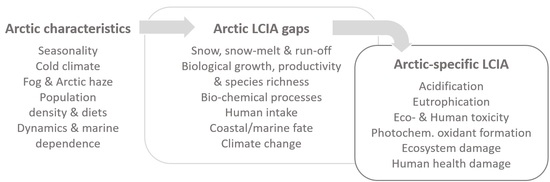
This study shows that there are indeed significant gaps in the application of the available LCIA methods in the Arctic context, owing to a number of Arctic features (Table 1). Examples of the LCA-relevant Arctic features include seasonality, cold climate, fog, precipitation, population density and diets, and marine dependence, which could potentially affect the results of impact pathway analysis in characterization modeling and impact assessment in LCA. Those Arctic-specific features and possible influences on LCA characterization modeling need to be considered in the development of future Arctic life cycle impact assessment.
In a generic context, our recommendations for future research on Arctic LCAs emphasize the following two aspects. Firstly, taking into account the characteristics of the Arctic region and better integrating Arctic science into sustainability assessment tools (such as LCA) would increase precision and thus the public acceptance of LCA as an environmental decision-making support tool. Poor inclusion of relevant Arctic characteristics in continental fate models hampers the use of LCA to support sustainable development for Arctic industry and society. Secondly, it is important to address gaps in the coverage of impact pathways, particularly in the poor modeling of marine environments. The mining LCA case study shows the importance of Arctic emissions to the global impact of copper from Arctic mining, stressing climate change, local air pollution, marine ecotoxicity, and human health impacts. However, there are clear gaps in characterization modeling to cover Arctic conditions, marine impacts and impact chains in LCA. The public debate on environmental issues in the high North has a strong marine focus, with the marine representing both an intrinsic value as well as huge commercial values to traditional marine industries and new marine and marine-based industries alike. Better representation of marine processes and recipients would greatly aid in the applicability of LCA to support environmental management of industrial activities, environmental policy development, and stakeholder dialogue on sustainable development in the Arctic.
Acknowledgments
The authors gratefully acknowledge financial support from the Northern Environmental Waste Management (EWMA) project, funded by the Research Council of Norway through NORDSATSNING (grant number 195160) and Eni Norge AS.
Author Contributions
Johan Berg Pettersen and Xingqiang Song conceived and designed the research, carried out the case study, made discussions and concluding remarks, and wrote the paper.
Conflicts of Interest
The authors declare no conflict of interest.
References
- Huntington, H.; Weller, G.; Bush, E.; Callaghan, T.V.; Kattsov, V.M.; Nuttall, M. An Introduction to the Arctic Climate Impact. In Arctic Climate Impact Assessment; Symon, C., Arris, L., Hea, B., Eds.; Cambridge University Press: Cambridge, UK, 2005; pp. 1–20. [Google Scholar]
- Jeffries, M.O.; Overland, J.E.; Perovich, D.K. The Arctic shifts to a new normal. Phys. Today 2013, 66, 35–40. [Google Scholar] [CrossRef]
- Arctic Monitoring and Assessment Programme (AMAP). Summary for Policy-Makers: Arctic Pollution Issues 2015; Arctic Monitoring and Assessment Programme (AMAP): Oslo, Norway, 2015. [Google Scholar]
- Quinn, P.K.; Shaw, G.; Andrews, E.; Dutton, E.G.; Ruoho-Airola, T.; Gong, S.L. Arctic haze: Current trends and knowledge gaps. Tellus B 2007, 59, 99–114. [Google Scholar] [CrossRef]
- Gautier, D.L.; Bird, K.J.; Charpentier, R.R.; Grantz, A.; Houseknecht, D.W.; Klett, T.R.; Moore, T.E.; Pitman, J.K.; Schenk, C.J.; Schuenemeyer, J.H.; et al. Assessment of Undiscovered Oil and Gas in the Arctic. Science 2009, 324, 1175–1179. [Google Scholar] [CrossRef] [PubMed]
- Van Dam, K.; Scheepstra, A.; Gille, J.; Stępień, A.; Koivurova, T. Mining in The European Arctic. In Strategic Assessment of Development of the Arctic: Assessment Conducted for the European Union; Stępień, A., Koivurova, T., Kankaanpää, P., Eds.; The Arctic Center, University of Lapland: Rovaniemi, Finland, 2014; pp. 87–99. [Google Scholar]
- Nørregaard, R.D.; Nielsen, T.G.; Møller, E.F.; Strand, J.; Espersen, L.; Møhl, M. Evaluating pyrene toxicity on Arctic key copepod species Calanus hyperboreus. Ecotoxicology 2014, 23, 163–174. [Google Scholar] [CrossRef] [PubMed]
- Curran, M.A. Life Cycle Assessment Student Handbook; Wiley: Hoboken, NJ, USA, 2015; ISBN 978-1-119-08354-2. [Google Scholar]
- International Organization for Standardization (ISO). ISO 14040: Environmental Management—Life Cycle Assessment—Principles and Framework; International Organization for Standardization (ISO): Geneva, Switzerland, 2006. [Google Scholar]
- Curran, M.A. Life Cycle Assessment: A review of the methodology and its application to sustainability. Curr. Opin. Chem. Eng. 2013, 2, 273–277. [Google Scholar] [CrossRef]
- Margni, M.; Curran, M.A. Life Cycle Impact Assessment. In Life Cycle Assessment Handbook: A Guide for Environmentally Sustainable Products; Curran, M.A., Ed.; John Wiley & Sons, Inc.: Somerset, NJ, USA, 2012; pp. 67–103. [Google Scholar]
- Woods, J.S.; Veltman, K.; Huijbregts, M.A.J.; Verones, F.; Hertwich, E.G. Towards a meaningful assessment of marine ecological impacts in life cycle assessment (LCA). Environ. Int. 2016, 89–90, 48–61. [Google Scholar] [CrossRef] [PubMed] [Green Version]
- Fava, J.; Consoli, F.; Denison, R.; Dickson, K.; Mohin, T.; Vigon, B. A Conceptual Framework for Life Cycle Impact Assessment; Society of Environmental Toxicology and Chemistry (SETAC): Brussels, Belgium, 1993. [Google Scholar]
- Potting, J.; Hauschild, M. Predicted Environmental Impact and Expected Occurance of Actual Enviornmental Impact, Part I: The linear nature of environmental impact from emissions in life-cycle assessment. Int. J. Life Cycle Assess. 1997, 2, 171–177. [Google Scholar] [CrossRef]
- Potting, J.; Hauschild, M.; Hauschild, M. Spatial Differentiation in Life Cycle Impact Assessment: A decade of method development to increase the environmental realism of LCIA. Int. J. Life Cycle Assess. 2006, 11, 11–13. [Google Scholar] [CrossRef]
- United Nations Environment Programme (UNEP). Global Guidance for Life Cycle Impact Assessment Indicators Volume 1; Frischknecht, R., Jolliet, O., Eds.; United Nations Environment Programme (UNEP): Nairobi, Kenya, 2016. [Google Scholar]
- European Commission-Joint Research Centre (EC-JRC). International Reference Life Cycle Data System (ILCD) Handbook-Recommendations for Life Cycle Impact Assessment in the European Context; European Commission-Joint Research Centre (EC-JRC): Luxemburg, 2011. [Google Scholar]
- Rosenbaum, R.K.; Bachmann, T.M.; Gold, L.S.; Huijbregts, M.A.J.; Jolliet, O.; Juraske, R.; Koehler, A.; Larsen, H.F.; MacLeod, M.; Margni, M.; et al. USEtox—The UNEP-SETAC toxicity model: Recommended characterisation factors for human toxicity and freshwater ecotoxicity in life cycle impact assessment. Int. J. Life Cycle Assess. 2008, 13, 532–546. [Google Scholar] [CrossRef]
- Bennett, D.; McKone, T.E.; Evans, J.S.; Nazaroff, W.W.; Margni, M.D.; Smith, K.R. Defining Intake Fraction. Environ. Sci. Technol. 2002, 36, 206A–211A. [Google Scholar] [CrossRef]
- Hofstetter, P. Perspectives in Life Cycle Impact Assessment: A Structured Approach to Combine Models of the Technosphere, Ecosphere and Valuesphere; Kluwer Academic Publishers: Dordrecht, The Netherlands, 1998. [Google Scholar]
- Potting, J.; Schöpp, W.; Blok, K.; Hauschild, M. Site-Dependent Life-Cycle Impact Assessment of Acidification. J. Ind. Ecol. 1998, 2, 63–87. [Google Scholar] [CrossRef]
- Van Zelm, R.; Huijbregts, M.A.J.; van De Meent, D. USES-LCA 2.0-a global nested multi-media fate, exposure, and effects model. Int. J. Life Cycle Assess. 2009, 14, 282–284. [Google Scholar] [CrossRef]
- Owsianiak, M.; Rosenbaum, R.K.; Huijbregts, M.A.J.; Hauschild, M.Z. Addressing geographic variability in the comparative toxicity potential of copper and nickel in soils. Environ. Sci. Technol. 2013, 47, 3241–3250. [Google Scholar] [CrossRef] [PubMed]
- Posch, M.; Seppälä, J.; Hettelingh, J.P.; Johansson, M.; Margni, M.; Jolliet, O. The role of atmospheric dispersion models and ecosystem sensitivity in the determination of characterisation factors for acidifying and eutrophying emissions in LCIA. Int. J. Life Cycle Assess. 2008, 13, 477–486. [Google Scholar] [CrossRef]
- Toffoletto, L.; Bulle, C.; Godin, J.; Reid, C.; Deschênes, L. LUCAS—A New LCIA Method Used for a Canadian-Specific Context. Int. J. Life Cycle Assess. 2007, 12, 93–102. [Google Scholar] [CrossRef]
- Finnveden, G.; Nilsson, M. Site-dependent life-cycle impact assessment in Sweden. Int. J. Life Cycle Assess. 2005, 10, 235–239. [Google Scholar] [CrossRef]
- Verones, F.; Henderson, A.D.; Laurent, A.; Ridoutt, B.; Ugaya, C.; Hellweg, S. LCIA framework and modelling guidance. In Global Guidance for Life Cycle Impact Assessment Indicators Volume 1; Frischknecht, R., Jolliet, O., Eds.; United Nations Environment Programme (UNEP): Nairobi, Kenya, 2016. [Google Scholar]
- Johnsen, F.M. Bridging Arctic environmental science and life cycle assessment: A preliminary assessment of regional scaling factors. Clean Technol. Environ. Policy 2014, 16, 1713–1724. [Google Scholar] [CrossRef]
- Arctic Monitoring and Assessment Programme (AMAP). Physical/Geographical Characteristics of the Arctic. In AMAP Assessment Report: Arctic Pollution Issues; Arctic Monitoring and Assessment Programme (AMAP): Oslo, Norway, 1998; pp. 9–24. [Google Scholar]
- Huntington, H.P. Arctic Flora and Fauna: Status and Conservation; Edita: Helsinki, Finland, 2001. [Google Scholar]
- Prowse, T.D.; Wrona, F.J.; Reist, J.D.; Hobbie, J.E.; Lévesque, L.M.J.; Vincent, W.F.; Gibson, J.J.; Hobbie, J.E.; Lévesque, L.M.J.; Vincent, W.F. General Features of the Arctic Relevant to Climate Change in Freshwater Ecosystems. Ambio 2006, 35, 330–338. [Google Scholar] [CrossRef]
- Przybylak, R. Cloudiness. In The Climate of the Arctic; Springer International Publishing: Basel, Switzerland, 2016; pp. 111–126. [Google Scholar]
- Holmes, R.M.; McClelland, J.W.; Peterson, B.J.; Tank, S.E.; Bulygina, E.; Eglinton, T.I.; Gordeev, V.V.; Gurtovaya, T.Y.; Raymond, P.A.; Repeta, D.J.; et al. Seasonal and Annual Fluxes of Nutrients and Organic Matter from Large Rivers to the Arctic Ocean and Surrounding Seas. Estuaries Coasts 2012, 35, 369–382. [Google Scholar] [CrossRef]
- Siron, R.; Sherman, K.; Skjoldal, H.R.; Hiltz, E. Ecosystem-Based Management in the Arctic Ocean: A Multi-Level Spatial Approach. Arctic 2008, 61, 86–102. [Google Scholar] [CrossRef]
- Bring, A.; Fedorova, I.; Dibike, Y.; Hinzman, L.; Mård, J.; Mernild, S.H.; Prowse, T.; Semenova, O.; Stuefer, S.L.; Woo, M.K. Arctic terrestrial hydrology: A synthesis of processes, regional effects, and research challenges. J. Geophys. Res. Biogeosci. 2016, 121, 621–649. [Google Scholar] [CrossRef]
- Kaste, Ø.; Rankinen, K.; Lepistö, A. Modelling impacts of climate and deposition changes on nitrogen fluxes in northern catchments of Norway and Finland. Hydrol. Earth Syst. Sci. 2004, 8, 778–792. [Google Scholar] [CrossRef]
- Arctic Monitoring and Assessment Programme (AMAP). Snow, Water, Ice and Permafrost. Summary for Policy-Makers; Arctic Monitoring and Assessment Programme (AMAP): Oslo, Norway, 2017. [Google Scholar]
- Chen, M.; Huang, Y.P.; Guo, L.D.; Cai, P.H.; Yang, W.F.; Liu, G.S.; Qiu, Y.S. Biological productivity and carbon cycling in the Arctic Ocean. Chin. Sci. Bull. 2002, 47, 1037–1040. [Google Scholar] [CrossRef]
- Loeng, H.; Brander, K.; Carmack, E.; Denisenko, S.; Drinkwater, K.; Hansen, B.; Kovacs, K.; Livingston, P.; McLaughlin, F.; Sakshaug, E. Marine Systems. In Arctic Cimate Impact Assessment; Cambridge University Press: Cambridge, UK, 2005; pp. 452–538. ISBN 0521865093. [Google Scholar]
- Darnis, G.; Robert, D.; Pomerleau, C.; Link, H.; Archambault, P.; Nelson, R.J.; Geoffroy, M.; Tremblay, J.E.; Lovejoy, C.; Ferguson, S.H.; et al. Current state and trends in Canadian Arctic marine ecosystems: II. Heterotrophic food web, pelagic-benthic coupling, and biodiversity. Clim. Chang. 2012, 115, 179–205. [Google Scholar] [CrossRef]
- Chapman, P.M.; Riddle, M.J. Toxic Effects of Contaminants in Polar Marine Environments. Environ. Sci. Technol. 2005, 39, 200A–207A. [Google Scholar] [CrossRef] [PubMed]
- Murray, J.L. Ecological Characteristics of the Arctic. In AMAP Assessment Report: Arctic Pollution Issues; Arctic Monitoring and Assessment Programme (AMAP): Oslo, Norway, 1998; pp. 117–140. [Google Scholar]
- Bejarano, A.C.; Gardiner, W.W.; Barron, M.G.; Word, J.Q. Relative sensitivity of Arctic species to physically and chemically dispersed oil determined from three hydrocarbon measures of aquatic toxicity. Mar. Pollut. Bull. 2017, 122, 316–322. [Google Scholar] [CrossRef] [PubMed]
- Chapman, P.M.; McDonald, B.G.; Kickham, P.E.; McKinnon, S. Global geographic differences in marine metals toxicity. Mar. Pollut. Bull. 2006, 52, 1081–1084. [Google Scholar] [CrossRef] [PubMed]
- Marcus Zamora, L.; King, C.K.; Payne, S.J.; Virtue, P. Sensitivity and response time of three common Antarctic marine copepods to metal exposure. Chemosphere 2015, 120, 267–272. [Google Scholar] [CrossRef] [PubMed]
- McMeans, B.C.; McCann, K.S.; Humphries, M.; Rooney, N.; Fisk, A.T. Food Web Structure in Temporally-Forced Ecosystems. Trends Ecol. Evol. 2015, 30, 662–672. [Google Scholar] [CrossRef] [PubMed]
- Wirta, H.K.; Vesterinen, E.J.; Hambäck, P.A.; Weingartner, E.; Rasmussen, C.; Reneerkens, J.; Schmidt, N.M.; Gilg, O.; Roslin, T. Exposing the structure of an Arctic food web. Ecol. Evol. 2015, 5, 3842–3856. [Google Scholar] [CrossRef] [PubMed]
- Heleniak, T.; Bogoyavlenskiy, D. Arctic Populations and Migration. In Arctic Human Development Report: Regional Processes and Global Linkages; Larsen, J.N., Fondahl, G., Eds.; Nordic Council of Ministers: Copenhagen, Denmark, 2013; pp. 53–104. [Google Scholar]
- Petrov, A.N.; BurnSilver, S.; Chapin, F.S.; Fondahl, G.; Graybill, J.; Keil, K.; Nilsson, A.E.; Riedlsperger, R.; Schweitzer, P.; Chapin, F.S., III; et al. Arctic sustainability research: Toward a new agenda. Polar Geogr. 2016, 39, 165–178. [Google Scholar] [CrossRef]
- Rasmussen, R.O.; Hovelsrud, G.K.; Gearheard, S. Community viability and adaptation. In Arctic Human Development Report: Regional Processes and Global Linkages; Larsen, J.N., Fondahl, G., Eds.; Nordic Council of Ministers: Copenhagen, Denmark, 2015. [Google Scholar]
- ArcticStat. Available online: http://www.arcticstat.org/ (accessed on 6 July 2017).
- Huntington, H.P. Peoples of the Arctic: Characteristics of Human Populations Relevant to Pollution Issues. In AMAP Assessment Report: Arctic Pollution Issues; Arctic Monitoring and Assessment Programme (AMAP): Oslo, Norway, 1998; pp. 141–183. [Google Scholar]
- Bjerregaard, P.; Aidt, E.C. Levevilkår, Livsstil og Helbred. Befolkningsundersøgelser i Grønland 2005–2009; Statens Institut for Folkesundhet: Copenhagen, Denmark, 2010; ISBN 9788778991676. [Google Scholar]
- Bjerregaard, P.; Curtis, T.; Senderovitz, F.; Christensen, U.; Pars, T. Levevilkår, Livsstil og Helbred i Grønland; Dansk Institut for Klinisk Epidemiologi (DIKE): Copenhagen, Denmark, 1995; ISBN 8789662741. [Google Scholar]
- Nobmann, E.D.; Byers, T.; Lanier, A.P.; Hankin, J.H.; Jackson, M.Y. The diet of Alaska Native adults: 1987–1988. Am. J. Clin. Nutr. 1992, 55, 1024–1032. [Google Scholar] [PubMed]
- Huijbregts, M.A.J.; Steinmann, Z.J.N.; Elshout, P.M.F.; Stam, G.; Verones, F.; Vieira, M.; Zijp, M.; Hollander, A.; van Zelm, R. ReCiPe2016: A harmonised life cycle impact assessment method at midpoint and endpoint level. Int. J. Life Cycle Assess. 2017, 22, 138–147. [Google Scholar] [CrossRef]
- Jolliet, O.; Margni, M.; Charles, R.; Humbert, S.; Payet, J.; Rebitzer, G.; Robenbaum, R.K. IMPACT 2002+: A New Life Cycle Impact Assessment Methodology. Int. J. Life Cycle Assess. 2003, 8, 324–330. [Google Scholar] [CrossRef]
- IMPACT World+. Available online: http://www.impactworldplus.org/en/ (accessed on 10 June 2017).
- LC-Impact: A Spatially Differentiated Life Cycle Impact Assessment Method. Available online: http://www.lc-impact.eu/ (accessed on 10 May 2017).
- Itsubo, N.; Sakagami, M.; Washida, T.; Kokubu, K.; Inaba, A. Weighting across safeguard subjects for LCIA through the application of conjoint analysis. Int. J. Life Cycle Assess. 2004, 9, 196–205. [Google Scholar] [CrossRef]
- Bare, J. TRACI 2.0: The tool for the reduction and assessment of chemical and other environmental impacts 2.0. Clean Technol. Environ. Policy 2011, 13, 687–696. [Google Scholar] [CrossRef]
- Cherubini, F.; Fuglestvedt, J.; Gasser, T.; Reisinger, A.; Cavalett, O.; Huijbregts, M.A.J.; Johansson, D.J.A.; Jørgensen, S.V.; Raugei, M.; Schivley, G.; et al. Bridging the gap between impact assessment methods and climate science. Environ. Sci. Policy 2016, 64, 129–140. [Google Scholar] [CrossRef]
- Levasseur, A. Climate Change. In Life Cycle Impact Assessment; Hauschild, M.Z., Huijbregts, M.A.J., Eds.; Springer: Dordrecht, The Netherlands, 2015; pp. 257–259. [Google Scholar]
- Addressing Climate Change in the Near Term: Short-Lived Climate Pollutants. Available online: http://www.c2es.org/science-impacts/short-lived-climate-pollutants (accessed on 26 July 2017).
- Myhre, G.; Shindell, D.; Bréon, F.M.; Collins, W.; Fuglestvedt, J.; Huang, J.; Koch, D.; Lamarque, J.F.; Lee, D.; Mendoza, B.; et al. Anthropogenic and Natural Radiative Forcing. In Climate Change 2013—The Physical Science Basis; Cambridge University Press: Cambridge, UK, 2013; pp. 659–740. [Google Scholar]
- Ødemark, K.; Dalsøren, S.B.; Samset, B.H.; Berntsen, T.K.; Fuglestvedt, J.S.; Myhre, G. Short-lived climate forcers from current shipping and petroleum activities in the Arctic. Atmos. Chem. Phys. 2012, 12, 1979–1993. [Google Scholar] [CrossRef] [Green Version]
- Quinn, P.K.; Stohl, A.; Arneth, A.; Berntsen, T.; Burkhart, J.F.; Christensen, J.; Flanner, M.; Kupiainen, K.; Lihavainen, H.; Shepherd, M.; et al. The Impact of Black Carbon on Arctic Climate; Arctic Monitoring and Assessment Programme (AMAP): Oslo, Norway, 2011. [Google Scholar]
- Flanner, M.G.; Zender, C.S.; Randerson, J.T.; Rasch, P.J. Present-day climate forcing and response from black carbon in snow. J. Geophys. Res. Atmos. 2007, 112. [Google Scholar] [CrossRef]
- Fiore, A.M.; Jacob, D.J.; Bey, I.; Yantosca, R.M.; Field, B.D.; Fusco, A.C.; Wilkinson, J.G. Background ozone over the United States in summer: Origin, trend, and contribution to pollution episodes. J. Geophys. Res. Atmos. 2002, 107. [Google Scholar] [CrossRef]
- Preiss, P. Photochemical Ozone Formation. In Life Cycle Impact Assessment; Hauschild, M.Z., Huijbregts, M.A.J., Eds.; Springer: Dordrecht, The Netherlands, 2015; pp. 115–138. [Google Scholar]
- Schaap, M.; Timmermans, R.M.A.; Roemer, M.; Boersen, G.A.C.; Builtjes, P.J.H.; Sauter, F.J.; Velders, G.J.M.; Beck, J.P. The LOTOS-EUROS model: Description, validation and latest developments. Int. J. Environ. Pollut. 2008, 32, 270–290. [Google Scholar] [CrossRef]
- Van Zelm, R.; Preiss, P.; van Goethem, T.; van Dingenen, R.; Huijbregts, M. Regionalized life cycle impact assessment of air pollution on the global scale: Damage to human health and vegetation. Atmos. Environ. 2016, 134, 129–137. [Google Scholar] [CrossRef] [Green Version]
- World Health Organization. Health Risks of Particulate Matter from Long-Range Transboundary Air Pollution; World Health Organization: Copenhagen, Denmark, 2006. [Google Scholar]
- Pijnappel, A. Statistical Post Processing of Model Output from the Air Quality Model LOTOS-EUROS; The Royal Netherlands Meteorological Institute (KNMI): De Bilt, The Netherlands, 2011. [Google Scholar]
- Humbert, S.; Fantke, P.; Jolliet, O. Particulate Matter Formation. In Life Cycle Impact Assessment; Hauschild, M.Z., Huijbregts, M.A.J., Eds.; Springer: Dordrecht, The Netherlands, 2015; pp. 97–113. [Google Scholar]
- Van Zelm, R.; Huijbregts, M.A.J.; den Hollander, H.A.; van Jaarsveld, H.A.; Sauter, F.J.; Struijs, J.; van Wijnen, H.J.; van de Meent, D. European characterization factors for human health damage of PM10 and ozone in life cycle impact assessment. Atmos. Environ. 2008, 42, 441–453. [Google Scholar] [CrossRef]
- Goedkoop, M.; Heijungs, R.; De Schryver, A.; Struijs, J.; van Zelm, R. ReCiPe 2008: A Life Cycle Impact Assessment Method Which Comprises Harmonised Category Indicators at the Midpoint and the Endpoint Level. Report I: Characterisation; Ministry of Housing, Spatial Planning and Environment: The Hague, The Netherlands, 2013. [Google Scholar]
- Humbert, S.; Marshall, J.D.; Shaked, S.; Spadaro, J.V.; Nishioka, Y.; Preiss, P.; McKone, T.E.; Horvath, A.; Jolliet, O. Intake fraction for particulate matter: Recommendations for life cycle impact assessment. Environ. Sci. Technol. 2011, 45, 4808–4816. [Google Scholar] [CrossRef] [PubMed]
- Van Zelm, R. Damage Modeling in Life Cycle Impact Assessment; Radboud University: Nijmegen, The Netherlands, 2010. [Google Scholar]
- Van Zelm, R.; Huijbregts, M.A.J.; van Jaarsveld, H.A.; Reinds, G.J.; De Zwart, D.; Struijs, J.; Van De Meent, D. Time horizon dependent characterization factors for acidification in life-cycle assessment based on forest plant species occurrence in Europe. Environ. Sci. Technol. 2007, 41, 922–927. [Google Scholar] [CrossRef] [PubMed]
- Seppälä, J.; Posch, M.; Johansson, M.; Hettelingh, J.-P. Country-dependent Characterisation Factors for Acidification and Terrestrial Eutrophication Based on Accumulated Exceedance as an Impact Category Indicator. Int. J. Life Cycle Assess. 2006, 11, 403–416. [Google Scholar] [CrossRef]
- Forsius, M.; Posch, M.; Aherne, J.; Reinds, G.J.; Christensen, J.; Hole, L. Assessing the impacts of long-range sulfur and nitrogen deposition on arctic and sub-arctic ecosystems. Ambio 2010, 39, 136–147. [Google Scholar] [CrossRef] [PubMed]
- Huijbregts, M.A.J.; Schöpp, W.; Verkuijlen, E.; Heijungs, R.; Reijnders, L. Spatially excplicit characterisation of acidifying and eutrophying air pollution in life-cycle assessment. J. Ind. Ecol. 2001, 4, 75–92. [Google Scholar] [CrossRef]
- Roy, P.O.; Deschênes, L.; Margni, M. Life cycle impact assessment of terrestrial acidification: Modeling spatially explicit soil sensitivity at the global scale. Environ. Sci. Technol. 2012, 46, 8270–8278. [Google Scholar] [CrossRef] [PubMed]
- Wet Deposition. Available online: http://wiki.seas.harvard.edu/geos-chem/index.php/Wet_deposition (accessed on 3 July 2017).
- Azevedo, L.B.; Roy, P.O.; Verones, F.; van Zelm, R.; Huijbregts, M.A.J. Terrestrial acidification. In LC-Impact Version 0.5: A Spatially Differentiated Life Cycle Impact Assessment Approach; Verones, F., Hellweg, S., Azevedo, L.B., Chaudhary, A., Cosme, N., Fantke, P., Goedkoop, M., Hauschild, M., Laurent, A., Mutel, C.L., et al., Eds.; European LC-IMPACT Project Report: Trondheim, Norway, 2016; Available online: http://www.lc-impact.eu (accessed on 7 September 2017).
- Roy, P.O.; Deschênes, L.; Margni, M. Uncertainty and spatial variability in characterization factors for aquatic acidification at the global scale. Int. J. Life Cycle Assess. 2014, 19, 882–890. [Google Scholar] [CrossRef]
- Hauschild, M.; Potting, J. Spatial Differentiation in LCA Impact Assessment—The EDIP2003 Methodology; Danish Environmental Protection Agency: Copenhagen, Denmark, 2005. [Google Scholar]
- Beusen, A.H.W.; Klepper, O.; Meinardi, C.R. Modelling the flow of nitrogen and phosphorus in Europe: From loads to coastal seas. Water Sci. Technol. 1995, 31, 141–145. [Google Scholar]
- Verones, F.; Hellweg, S.; Azevedo, L.B.; Laurent, A.; Mutel, C.L.; Pfister, S. Freshwater eutrophication. In LC-Impact Version 0.5: A Spatially Differentiated Life Cycle Impact Assessment Approach; Verones, F., Hellweg, S., Azevedo, L.B., Chaudhary, A., Cosme, N., Fantke, P., Goedkoop, M., Hauschild, M., Laurent, A., Mutel, C.L., et al., Eds.; European LC-IMPACT Project Report: Trondheim, Norway, 2016; Available online: http://www.lc-impact.eu/ (accessed on 7 September 2017).
- Azevedo, L.B.; Henderson, A.D.; van Zelm, R.; Jolliet, O.; Huijbregts, M.A.J. Assessing the importance of spatial variability versus model choices in life cycle impact assessment: The case of freshwater eutrophication in Europe. Environ. Sci. Technol. 2013, 47, 13565–13570. [Google Scholar] [CrossRef] [PubMed]
- Gandhi, N.; Huijbregts, M.A.J.; van de Meent, D.; Peijnenburg, W.J.G.M.; Guinee, J.; Diamond, M.L. Implications of geographic variability on Comparative Toxicity Potentials of Cu, Ni and Zn in freshwaters of Canadian ecoregions. Chemosphere 2011, 82, 268–277. [Google Scholar] [CrossRef] [PubMed]
- Henderson, A.D.; Hauschild, M.Z.; van De Meent, D.; Huijbregts, M.A.J.; Larsen, H.F.; Margni, M.; McKone, T.E.; Payet, J.; Rosenbaum, R.K.; Jolliet, O. USEtox fate and ecotoxicity factors for comparative assessment of toxic emissions in life cycle analysis: Sensitivity to key chemical properties. Int. J. Life Cycle Assess. 2011, 16, 701–709. [Google Scholar] [CrossRef]
- Rosenbaum, R.K. Ecotoxicity. In Life Cycle Impact Assessment; Hauschild, Z.M., Huijbregts, A.J.M., Eds.; Springer: Dordrecht, The Netherlands, 2015; pp. 139–162. [Google Scholar]
- Stewart, D.M.; Holt, D.P.; Rouwette, M.R. Application of LCA in Mining and Minerals Processing-Current Programs and Noticeable Gaps. In Life Cycle Assessment Handbook; Curran, M.A., Ed.; John Wiley & Sons, Inc.: Somerset, NJ, USA, 2012; pp. 267–289. [Google Scholar]
- Hauschild, M.Z.; Goedkoop, M.; Guinée, J.; Heijungs, R.; Huijbregts, M.; Jolliet, O.; Margni, M.; De Schryver, A.; Humbert, S.; Laurent, A.; et al. Identifying best existing practice for characterization modeling in life cycle impact assessment. Int. J. Life Cycle Assess. 2013, 18, 683–697. [Google Scholar] [CrossRef]
- Mcfarlin, K.M.; Perkins, R.A.; Gardiner, W.W.; Word, J.D.; Word, J.Q. Toxicity of Physically and Chemically Dispersed Oil to Selected Arctic Species. Int. Oil Spill Conf. Proc. 2011, 2011, abs149. [Google Scholar] [CrossRef]
- Chapman, P.M. Toxicity delayed in cold freshwaters? J. Great Lakes Res. 2016, 42, 286–289. [Google Scholar] [CrossRef]
- Hjorth, M.; Nielsen, T.G. Oil exposure in a warmer Arctic: Potential impacts on key zooplankton species. Mar. Biol. 2011, 158, 1339–1347. [Google Scholar] [CrossRef]
- Payne, S.J.; King, C.K.; Zamora, L.M.; Virtue, P. Temporal changes in the sensitivity of coastal Antarctic zooplankton communities to diesel fuel: A comparison between single- and multi-species toxicity tests. Environ. Toxicol. Chem. 2014, 33, 882–890. [Google Scholar] [CrossRef] [PubMed]
- Nussir ASA. Nussir Mine and Ulveryggen Mine Preliminary Economic Assessment (PEA); Nussir ASA: Kvalsund, Norway, 2014. [Google Scholar]
- Song, X.; Pettersen, J.B.; Pedersen, K.B.; Røberg, S. Comparative life cycle assessment of tailings management and energy scenarios for a copper ore mine: A case study in Northern Norway. J. Clean. Prod. 2017, 164, 892–904. [Google Scholar] [CrossRef]
- Shindell, D.; Faluvegi, G. Climate response to regional radiative forcing during the twentieth century. Nat. Geosci. 2009, 2, 294–300. [Google Scholar] [CrossRef]
- Svendsen, H. Physical oceanography of coupled fjord-coast systems in northern Norawy with special focus on frontal dynamics and tides. In Ecology of Fjords and Coastal Waters; Elsevier: New York, NY, USA, 1995; pp. 149–164. [Google Scholar]
- Roy, P.O.; Huijbregts, M.; Deschênes, L.; Margni, M. Spatially-differentiated atmospheric source-receptor relationships for nitrogen oxides, sulfur oxides and ammonia emissions at the global scale for life cycle impact assessment. Atmos. Environ. 2012, 62, 74–81. [Google Scholar] [CrossRef]
- Gandhi, N.; Diamond, M.L.; Huijbregts, M.A.J.; Guinée, J.B.; Peijnenburg, W.J.G.M.; van De Meent, D. Implications of considering metal bioavailability in estimates of freshwater ecotoxicity: Examination of two case studies. Int. J. Life Cycle Assess. 2011, 16, 774–787. [Google Scholar] [CrossRef]
Figure 1.
Arctic and subarctic floristic boundary to delimit the terrestrial Arctic by the treeline [29].
Figure 1.
Arctic and subarctic floristic boundary to delimit the terrestrial Arctic by the treeline [29].

Figure 2.
(a) Location of the Nussir copper ore mine on Google Map; and (b) a natural landscape view of the Nussir mineral processing plant adjacent to Repparfjorden, northern Norway.
Figure 2.
(a) Location of the Nussir copper ore mine on Google Map; and (b) a natural landscape view of the Nussir mineral processing plant adjacent to Repparfjorden, northern Norway.

Figure 3.
(a) Midpoint; and (b) endpoint life cycle contribution analysis results of Arctic and non-Arctic emissions using the ReCiPe (H) method (CC, climate change; TA, terrestrial acidification; FE, freshwater eutrophication; ME, marine eutrophication; HT, human toxicity; POF, photochemical oxidant formation; PMF, particulate matter formation; TET, terrestrial ecotoxicity; FET, freshwater ecotoxicity; MET, marine ecotoxicity).


Table 1.
Research gaps and demand for future Arctic LCA (ACID, acidification; EUTR, eutrophication; ECOTOX, ecotoxicity; HUMTOX, human toxicity).
Table 1.
Research gaps and demand for future Arctic LCA (ACID, acidification; EUTR, eutrophication; ECOTOX, ecotoxicity; HUMTOX, human toxicity).
| Arctic Characteristics | Gaps in Causality Chains (Impact Pathways) | Arctic-Dependent Impacts |
|---|---|---|
| Seasonality | Snow melt and spring run-off | ACID, EUTR, metal toxicity |
| Short growth season | ACID, EUTR, ECOTOX | |
| Seasonal lipid storage | ACID, EUTR, ECOTOX, HUMTOX | |
| Photochemistry (sun-hours and UV) | Photochemical oxidant formation | |
| Migratory behavior | Ecosystem damage, toxicity | |
| Seasonal food webs | Ecosystem damage, toxicity | |
| Cold climate | BC and PM on snow (albedo) | Climate change |
| Bio-chemical process rates | ACID, EUTR, ECOTOX | |
| Biological productivity | ECOTOX | |
| Species richness Ecosystem sensitivity | Ecosystem damage Ecosystem damage | |
| Fog and Arctic haze | Photochemistry (sun-hours and UV) | Photochemical oxidant formation |
| Precipitation | Precipitation rate, snow vs. rain | ACID, EUTR, toxicity |
| Population density | Human intake fraction | Human toxicity |
| Diets | Human intake fraction | Human toxicity |
| Marine dependence | Marine-freshwater interaction and near-shore/coastal fate processes | ACID, EUTR, ECOTOX, HUMTOX |
| Dynamics | Climate change | Climate change, ACID, EUTR, ECOTOX, HUMTOX |
© 2017 by the authors. Licensee MDPI, Basel, Switzerland. This article is an open access article distributed under the terms and conditions of the Creative Commons Attribution (CC BY) license (http://creativecommons.org/licenses/by/4.0/).
Share and Cite
MDPI and ACS Style
Pettersen, J.B.; Song, X. Life Cycle Impact Assessment in the Arctic: Challenges and Research Needs. Sustainability 2017, 9, 1605. https://doi.org/10.3390/su9091605
AMA Style
Pettersen JB, Song X. Life Cycle Impact Assessment in the Arctic: Challenges and Research Needs. Sustainability. 2017; 9(9):1605. https://doi.org/10.3390/su9091605
Chicago/Turabian StylePettersen, Johan Berg, and Xingqiang Song. 2017. "Life Cycle Impact Assessment in the Arctic: Challenges and Research Needs" Sustainability 9, no. 9: 1605. https://doi.org/10.3390/su9091605
Note that from the first issue of 2016, this journal uses article numbers instead of page numbers. See further details here.