“Group Inversion Approach” for Detection of Soil Moisture Temporal-Invariant Locations


Abstract
:1. Introduction
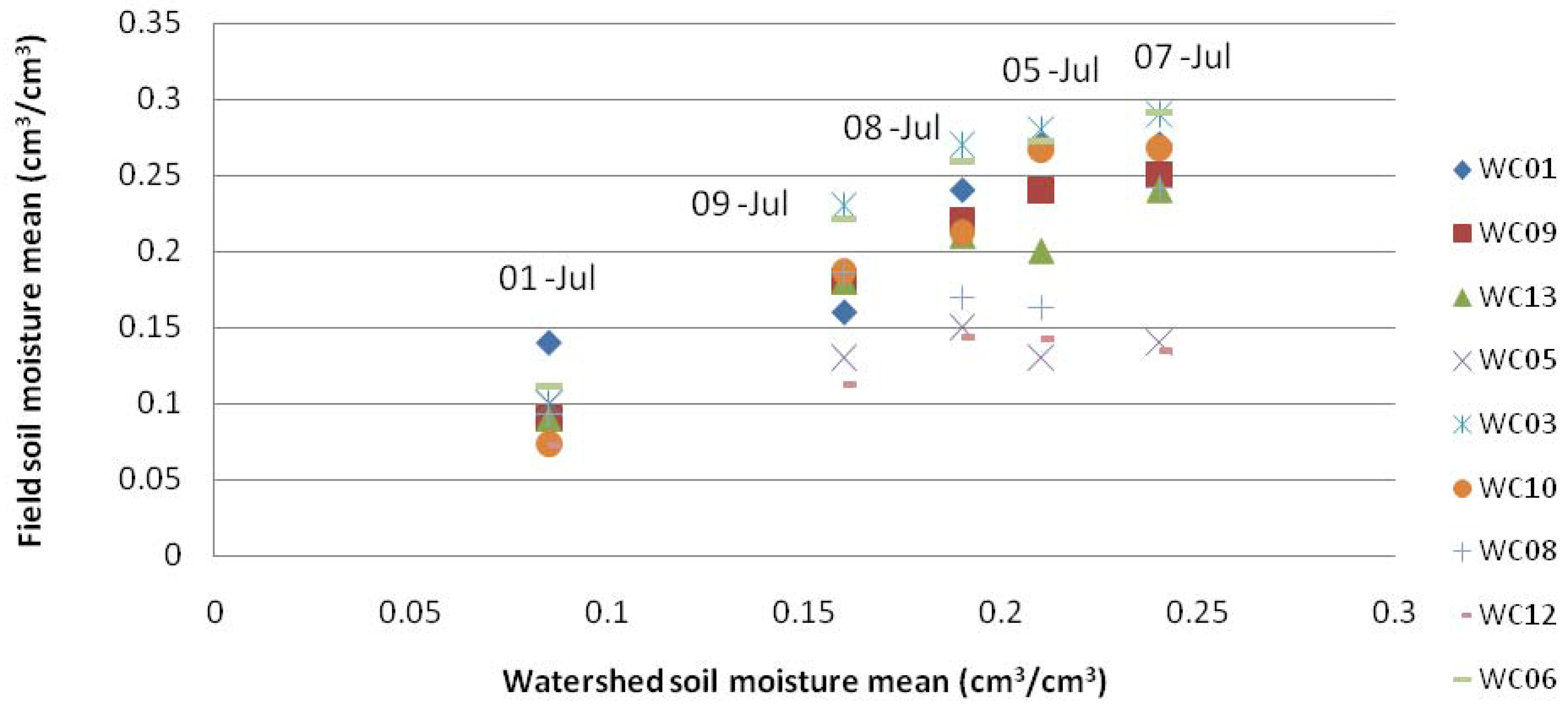
2. Experimental Data Sets
- -
- the number of fields that were considered in the experiment with different level of soil and vegetation moisture;
- -
- the acquisition of both radar and optical data and the extensive ground measurements carried out within each field.

| Fields | Roughness range | Volumetric soil moisture range | Vegetation | Biomass range (kg/m2) | Vegetation water content (kg/m2) |
|---|---|---|---|---|---|
| WC01 | 0.67 cm ≤ s ≤ 2.14 cm1.55 cm ≤ l ≤ 17.68 cm | 14% ≤ mv ≤ 27% | Corn | 2.17–7.46 | 3.50–4.70 |
| WC03 | 0.34 cm ≤ s ≤ 0.72 cm 1.40 cm ≤ l ≤ 13.05 cm | 11% ≤ mv ≤ 29% | Soybean | 0.13–0.41 | 0.36–0.88 |
| WC05 | 0.67 cm ≤ s ≤ 1.83 cm3.48 cm ≤ l ≤ 5.92 cm | 10% ≤ mv ≤ 16% | Corn | 1.14–2.36 | 3.70–4.76 |
| WC06 | 0.37 cm ≤ s ≤ 0.73 cm3.06 cm ≤ l ≤ 10.55 cm | 9% ≤ mv ≤ 24% | Corn | 0.35–2.23 | 3.88–4.61 |
| WC08 | 0.85 cm ≤ s ≤ 2.56 cm2.32 cm ≤ l ≤ 19.19 cm | 9% ≤ mv ≤ 24% | Corn | 1.06–1.62 | 3.66–4.78 |
| WC09 | 0.41 cm ≤ s ≤ 1.10 cm1.91 cm ≤ l ≤ 14.74 cm | 9 % ≤ mv ≤ 25% | Soybean | 0.28–0.60 | 0.45–0.92 |
| WC010 | 0.41 cm ≤ s ≤ 1.10 cm5.15 cm ≤ l ≤ 16.06 cm | 7% ≤ mv ≤ 27% | Soybean | 0.21–0.75 | 0.74–1.28 |
| WC012 | 0.64 cm ≤ s ≤ 1.65 cm8.17 cm ≤ l ≤ 16.94 cm | 7% ≤ mv ≤ 14% | Soybean | 1.06–2.32 | 3.50–4.60 |
| WC013 | 0.33 cm ≤ s ≤ 1.35cm0.47 cm ≤ l ≤ 11.17 cm | 10% ≤ mv ≤ 24% | Soybean | 0.10–0.42 | 0.29–0.66 |
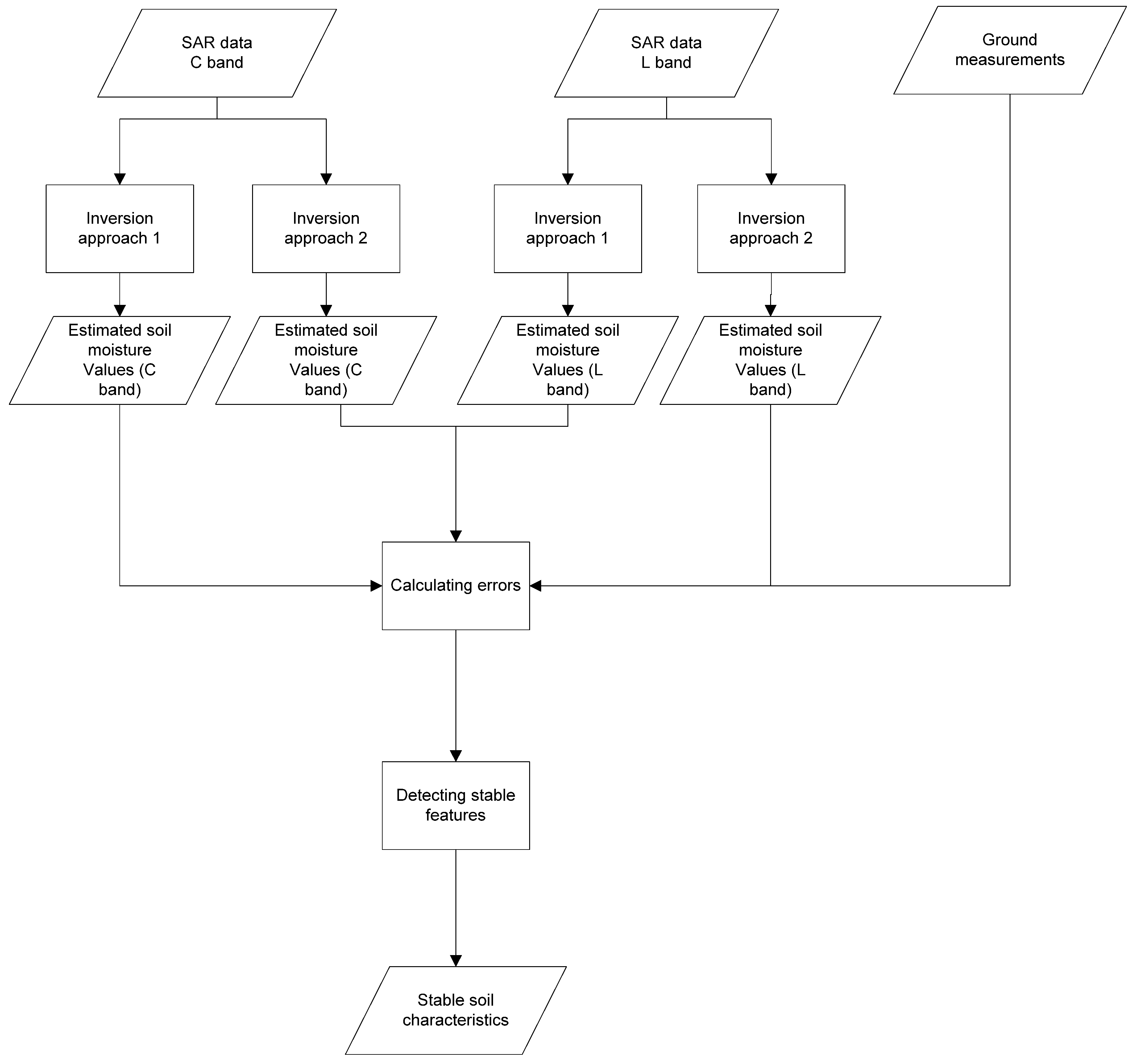
3. The Group Inversion Approach

3.1. The Bayesian approach
3.2. The empirical approach
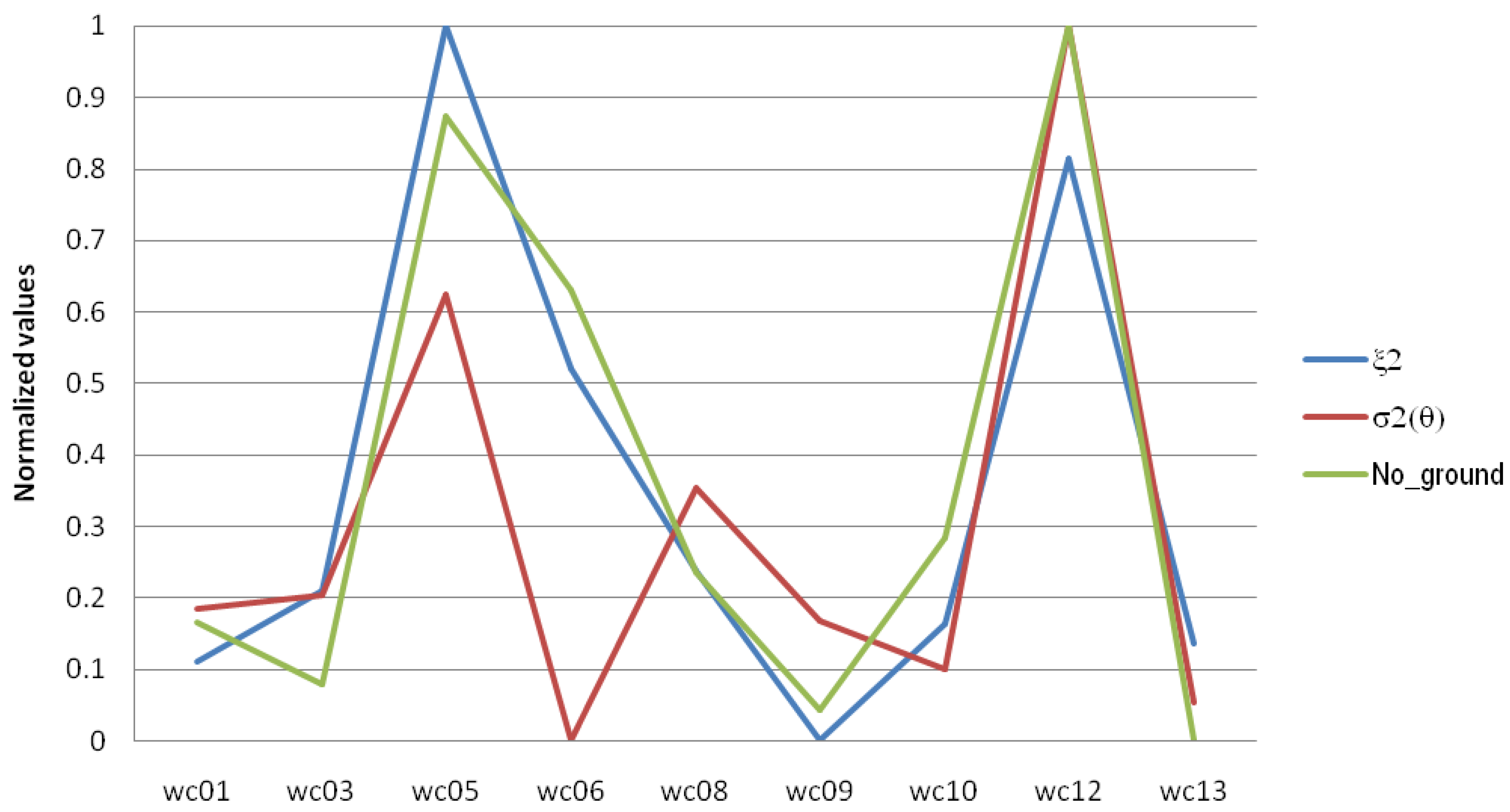
3.3. The Group Inversion Approach: Basic Theory
- -
- st(x,y), that represents the spatial distribution of soil moisture detected by the SAR sensor; in this case the main hypothesis is that the soil moisture patterns are detected by the radar backscatter [16]. To reduce the effect of speckle, the images have been multi-looked;
- -
- gt(x,y), that represents the spatial distribution of soil moisture detected by the ground measurements;
- -
- mt(x,y) that is the ‘real’ spatial distribution of soil moisture within the considered area.
- -
- mS,t: is the average of the SAR-inferred soil moisture values;
- -
- mG,t: is the average of the ground point measurements of soil moisture;
- -
- Vart(0): is the variance of the ground point measurements of soil moisture.
4. Results
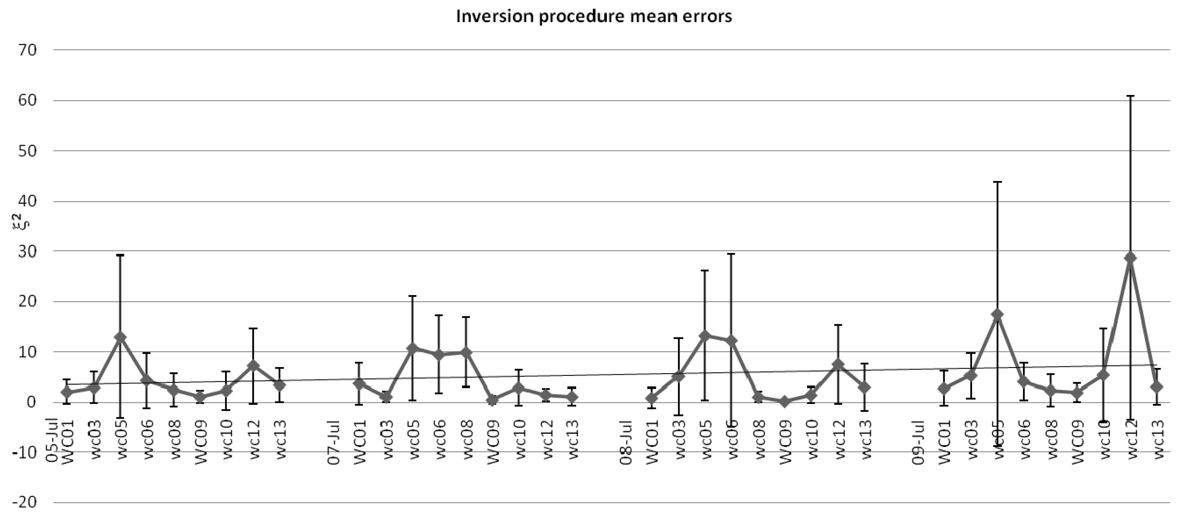
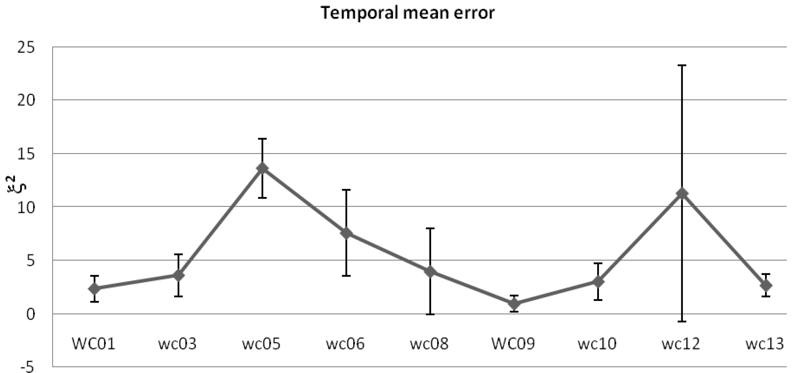
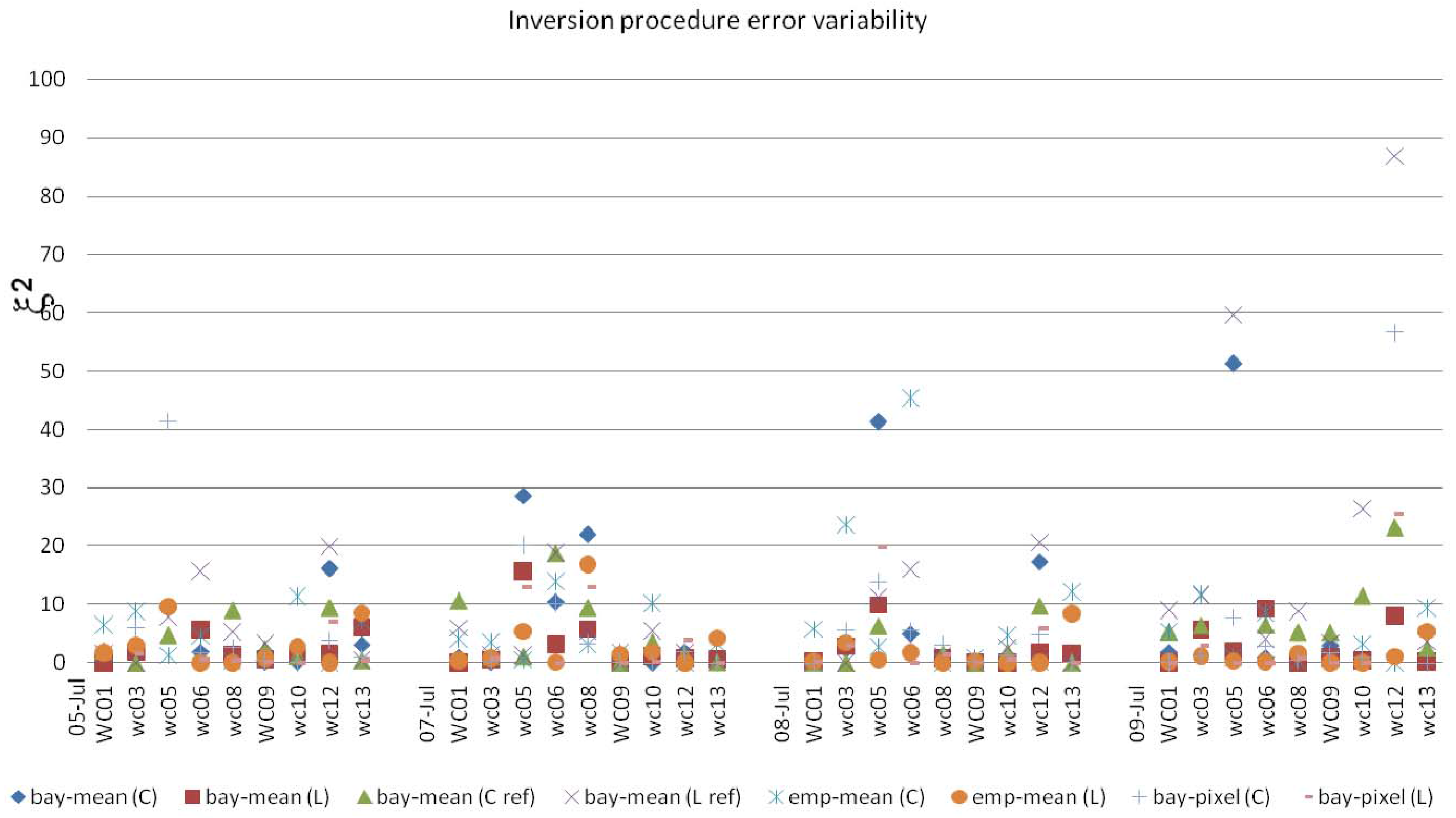
4.1. Results from the Group Inversion Approach
- -
- Bay-mean (C): the Bayesian approach applied to C band data on mean backscattering coefficients for each field,
- -
- Bay-mean (L): the Bayesian approach applied to L band data on mean backscattering coefficients for each field,
- -
- Bay-mean (Cref): the Bayesian approach applied to L band data on mean backscattering coefficients for each field. The estimates are compared with the estimates derived from the inversion approach applied to C band and not to ground measurements,
- -
- Bay-mean (Lref): the Bayesian approach applied to C band data on mean backscattering coefficients for each field. The estimates are compared with the estimates derived from the inversion approach applied to L band and not to ground measurements,
- -
- Emp-mean (C): the empirical approach applied to C band data on mean backscattering coefficients for each field,
- -
- Emp-mean (L): the empirical approach applied to L band data on mean backscattering coefficients for each field,
- -
- Bay-pixel (C): the Bayesian approach applied to C band data on a pixel basis and then averaging the results for each field,
- -
- Bay-pixel (L): the Bayesian approach applied to L band data on a pixel basis and then averaging the results for each field.


| Bias (cm3/cm3) | R2 | Slope | RMSE (cm3/cm3) | |
|---|---|---|---|---|
| WC01 | 0.04 | 0.84 | 0.96 | 0.044 |
| WC05 | 0.08 | 0.68 | 0.26 | 0.062 |
| WC09 | 0.004 | 0.97 | 1.08 | 0.021 |
| WC13 | 0.018 | 0.95 | 0.94 | 0.013 |
| WC03 | 0.007 | 0.935 | 1.281 | 0.061 |
| WC10 | 0.032 | 0.964 | 1.326 | 0.033 |
| WC08 | 0.03 | 0.772 | 0.792 | 0.026 |
| WC12 | 0.08 | 0.68 | 0.261 | 0.063 |
| WC06 | 0.02 | 0.971 | 1.191 | 0.056 |
4.2. Comparison between the GIA and Traditional Methodology Results
5. Conclusions and Future Developments
- -
- the field stable features can be estimated from the SAR images directly;
- -
- the comparison between the soil moisture estimates reveals the same behavior of the comparison between soil moisture estimates and soil moisture ground measurements;
- -
- this analysis can be useful in order to improve and better understand the upscaling and downscaling processing when passing from local to areal soil moisture estimation and vice versa;
- -
- In fact, an important application of this analysis is that starting from these stable fields can be inferred information of soil moisture on wider area. On the contrary, starting from images with coarse resolution such as scatterometer images, information at local scale can be obtained. This procedure may help in extrapolating local scale phenomena to regional and global scale by considering their spatial variability.
References and Notes
- Beven, K.J. Rainfall-Runoff Modeling: The Primer; John Wiley & Sons: Chichester, UK, 2001. [Google Scholar]
- Moran, M.S.; Hymer, D.C.; Qi, J.; Sano, E.E. Soil moisture evaluation using multi-temporal Synthetic Aperture Radar (SAR) in semiarid rangeland. Agr. For. Meteo. 2000, 105, 69–80. [Google Scholar] [CrossRef]
- Cosh, M.H.; Jackson, T.J.; Bindlish, R.; Prueger, J.H. Watershed scale temporal and spatial stability of soil moisture and its role in validating satellite estimates. Remote Sens. Environ. 2004, 92, 427–435. [Google Scholar] [CrossRef]
- Vachaud, G.; Passerat de Silans, A.; Balabanis, P.; Vauclin, M. Temporal stability of spatially measured soil water probability density function. Soil Sci. Soc. Am. J. 1985, 49, 822–828. [Google Scholar] [CrossRef]
- Grayson, R.B.; Western, A.W. Towards areal estimation of soil water content from point measurements: time and space stability of mean response. J. Hydrol. 1998, 207, 68–82. [Google Scholar] [CrossRef]
- Kachanosky, R.G.; de Jong, E. Scale dependence and the temporal persistence of spatial pattern of soil water storage. Water Resour. Res. 1988, 24, 85–91. [Google Scholar] [CrossRef]
- Gòmez-Plaza, A.; Alvarez-Rogel, J.; Alabaladejo, J.; Castillo, V.M. Spatial patterns and temporal stability of soil moisture across a range of scales in a semi-arid environment. Hydro. Process 2000, 14, 1261–1277. [Google Scholar] [CrossRef]
- Martinez-Fernandez, J.; Ceballos, A. Temporal stability of soil moisture in a large field experiment in Spain. Soil Sci. Soc. Am. J. 2003, 67, 1647–1656. [Google Scholar] [CrossRef]
- Wilson, D.J.; Western, A.W.; Grayson, R.B. Identifying and quantifying sources of variability in temporal and spatial soil moisture observations. Water Resour. Res. 2003, 40, W02507. [Google Scholar] [CrossRef]
- van Zyl, J.; Carande, R.; Lou, Y.; Miller, T.; Wheeler, K. The NASA/JPL three-frequency polarimetric AIRSAR system. IEEE IGARSS Dig. 1992, 1, 649–651. [Google Scholar]
- Notarnicola, C.; Angiulli, M.; Posa, F. Use of radar and optical remotely sensed data for soil moisture retrieval over vegetated areas. IEEE Trans. Geosci. Remote Sens. 2006, 44, 925–935. [Google Scholar] [CrossRef]
- Notarnicola, C.; Posa, F. Inferring vegetation water content from C and L band images. IEEE Trans. Geosci. Remote Sens. 2007, 45, 3165–3171. [Google Scholar] [CrossRef]
- Chen, D.; Jackson, T.J.; Li, F.; Cosh, M.H.; Walthall, C.; Anderson, M. Estimation of vegetation water content for corn and soybeans with a normalized difference water index (NDWI) using Landsat Thematic Mapper data. In Proceedings of IGARSS, Toulouse, France, 2003; pp. 2853–2856.
- Dubois, P.; van Zyl, J.J.; Engman, T. Measuring soil moisture with imaging radar. IEEE Trans. Geosci. Remote Sens. 1995, 33, 916–926. [Google Scholar] [CrossRef]
- Settle, J. On the use of remotely sensed data to estimate spatially averaged geophysical variables. IEEE Trans. Geosci. Remote Sens. 2004, 42, 620–631. [Google Scholar] [CrossRef]
- Wagner, W.; Pathe, C; Doubkova, M.; Sable, D.; Bartsch, A.; Hasenauer, S.; Bloeschl, G.; Scipal, K.; Martinez-Fernandez, J.; Loew, A. Temporal Stability of soil moisture and radar backscatter observed by the Advanced Synthetic Aperture Radar (ASAR). Sensors 2008, 8, 1174–1197. [Google Scholar] [CrossRef]
- Mohanty, B.P.; Skaggs, T.H. Spatial-temporal evolution and time-stable characteristics of soil moisture with remote sensing footprints with varying soil, slope, and vegetation. Adv. Water Resour. 2001, 24, 1051–1067. [Google Scholar] [CrossRef]
- Jacobs, J.M.; Mohanty, B.P.; Hsu, E.; Miller, D. SMEX02: field scale variability, time stability and similarity of soil moisture. Remote Sens. Environ. 2004, 92, 436–446. [Google Scholar] [CrossRef]
- Martinez-Fernandez, J.; Ceballos, A. Mean soil moisture estimation using temporal stability analysis. J. Hydrol. 2005, 312, 28–38. [Google Scholar] [CrossRef]
© 2009 by the authors; licensee Molecular Diversity Preservation International, Basel, Switzerland. This article is an open-access article distributed under the terms and conditions of the Creative Commons Attribution license (http://creativecommons.org/licenses/by/3.0/).
Share and Cite
Notarnicola, C. “Group Inversion Approach” for Detection of Soil Moisture Temporal-Invariant Locations. Remote Sens. 2009, 1, 1338-1352. https://doi.org/10.3390/rs1041338
Notarnicola C. “Group Inversion Approach” for Detection of Soil Moisture Temporal-Invariant Locations. Remote Sensing. 2009; 1(4):1338-1352. https://doi.org/10.3390/rs1041338
Chicago/Turabian StyleNotarnicola, Claudia. 2009. "“Group Inversion Approach” for Detection of Soil Moisture Temporal-Invariant Locations" Remote Sensing 1, no. 4: 1338-1352. https://doi.org/10.3390/rs1041338