Photogrammetric Methodology for the Production of Geomorphologic Maps: Application to the Veleta Rock Glacier (Sierra Nevada, Granada, Spain)

Abstract

In this paper we present a stereo feature-based method using SIFT (Scale-invariant feature transform) descriptors. We use automatic feature extractors, matching algorithms between images and techniques of robust estimation to produce a DTM (Digital Terrain Model) using convergent shots of a rock glacier.The geomorphologic structure observed in this study is the Veleta rock glacier (Sierra Nevada, Granada, Spain). This rock glacier is of high scientific interest because it is the southernmost active rock glacier in Europe and it has been analyzed every year since 2001. The research on the Veleta rock glacier is devoted to the study of its displacement and cartography through geodetic and photogrammetric techniques.

1. Introduction

The study of rock glaciers in high-mountain zones requires the production of detailed maps for the analysis of their evolution and behaviour through time. Using geomatic techniques (geodesy, global positioning system, photogrammetry) it is possible to study the dynamics of geomorphologic structures with high precision. In order to obtain 3D reconstructions in rock glaciers, conventional photogrammetry (metric camera and normal shots) and cheaper methods (semi-metric cameras and convergent photographs) can be used [1,2,3,4], but we aim for a more automatic method.

Obtaining detailed maps (cartography) in rock glaciers is difficult, because the use of flights to obtain photogrammetric images in these areas is expensive. Our aim is to develop a quick and cheap method to obtain enough 3D points to create a detailed DTM. Thus, two methodological goals are considered:

• Cartographic representation of the rock glacier, for example at a scale of 1/1,000 with a margin of error in the points of less than ±20 cm. This is the main objective of this study.
• Determination of the glacier dynamics through the time. Currently, we are working in this new methodology.

To fulfill these goals we use computer vision techniques to automatically detect as many points as possible of the natural environment which is specific to our example Veleta rock glacier. The application of computer vision techniques in this field has the following objectives:

• The creation of a Digital Terrain Model (DTM) with enough points in order to obtain a geomorphic map of the Veleta rock glacier.
• Replacing costly photogrammetric flights using planes with less expensive photographs taken from the top of the surrounding mountains, or using balloons or hang-gliders.
• Elimination of extensive office work by a human operator in obtaining 3D points or contour lines by replacing photogrammetric restitution with an automatic method, which also eliminates human errors.

2. Characteristic of the Veleta Rock Glacier

The Veleta rock glacier is located in “Sierra Nevada” (37°N–3°W) in a cirque at the bottom of Mount “Veleta” (3,398 m. a.s.l.). Sierra Nevada is a National Park at the south of Spain (Figure 1a). This mountain is very vulnerable to gelifraction which results in much more rock material on the Veleta rock glacier. The Veleta rock glacier forms an open figure “╗” (Figure 1b). Its source is attached to the wall of the “Corral” and continues in a northern direction and later extends to the west direction. It has an average slope of 20º, with the front at 3,090 m. a.s.l. and the root at 3,175 m. a.s.l. It is a tongue-shaped rock glacier 35 m wide and 109 m long [5].

The Veleta rock glacier has horizontal and vertical displacement with volumetric changes which have been verified through geodetic measurements over an eight year period (2001–2008). During this period the average dynamic of the rock glacier was 0.40/0.60 m in planimetry and −2.10/−2.60 m in altimetry [1].

Figure 1. (a). Veleta rock glacier situation; (b). Close view of the glacier from Mount Veleta.

Figure 1. (a). Veleta rock glacier situation; (b). Close view of the glacier from Mount Veleta.

3. Geomatic Methods

Several geomatic techniques can be employed to study any kind of rock glacier: Interferometry radar, laser scanner, geodesy (angle and distance measurements), levelling (geometric, trigonometric), Global Positioning System (GPS), photogrammetry (aerial, terrestrial, close range) [6,7,8]. In the case of Veleta rock glacier, the geodetic techniques (high precision total station), GPS and close range photogrammetry have been used [1]. The orography around the Veleta rock glacier (300 m high walls) and the cost make the application of some geomatic techniques difficult.

Some authors have used geodetic techniques and aerial photogrammety to obtain maps or to measure the glacier dynamics [3,9,10,11]. The advantage of the photogrammetry (aerial, terrestrial) over the geodesy is that photogrammetry can show the position of many points (photographic information), and it makes collecting information in the field much faster than geodesy [12,13].

3.1. Geodetic Survey and GPS

On the surface of the Veleta rock glacier, 20 control points were installed to monitor the glacier dynamics. These control points (iron rods) are measured every year to observe glacier dynamics and are also used for the photogrammetric process.

High precision topographic measurements were performed using a total station and a GPS. The total station is placed on the stable lateral moraine of the Veleta rock glacier and the maximum distance between the survey stations and the control points is 180 meters. The GPS method used is “RTK static”. So, a receiver is fixed on a point of known coordinates (X,Y,Z) and the other receiver is successively placed at the iron rods for 1 minute to ensure that every point has a spatial precision or GDOP less than 3 cm [14]. The control points for photogrammetry are the same points used for the monitoring of the dynamics of the rock glacier in order to reduce the time of data collection (Figure 2a).

Figure 2. (a) Photogrammetric control point; (b) Photogrametric shots from mount Veleta towards the rock glacier.

Figure 2. (a) Photogrammetric control point; (b) Photogrametric shots from mount Veleta towards the rock glacier.

3.2. Close range Photogrammetry (Conventional Photogrammetry)

A calibrated camera should be used to apply a photogrammetric general method and then the principal point, the focal length, the grid reseau coordinates and the lens distortion are known.

Figure 3. (a) Geometry of normal photogrammetry; (b) Geometry of convergent images. O₁ and O₂ are the centres of projection of the photographs.

Figure 3. (a) Geometry of normal photogrammetry; (b) Geometry of convergent images. O₁ and O₂ are the centres of projection of the photographs.

In the general aerial photogrammetric method, the cameras are placed in the normal configuration in a vertical direction in such a way that the optical axes of both photographs are parallel and perpendicular to the baseline (Figure 3a). This can be done with a plane flight but it cannot be done by hand in the Veleta rock glacier. Here, the operator is on the Veleta peak with the camera in hand on an uneven surface (Figure 2b). The images obtained have a convergent geometry (Figure 3b), and we take advantage of the epipolar geometry concept to deal with these convergent photographs. We have taken several photographs from which we have selected pairs to carry out the photogrammetric process using a stereoplotter.

The photogrammetric method of restitution to obtain the internal, relative and absolute orientations was difficult and it took several trials [15,16]. This is because the traditional restitution method is designed to work with image pairs in normal or quasi-normal configuration with parallel optical axis.

In summary, the general photogrammetric method used to obtain the map of the Veleta rock glacier involved the following issues:

• Method of photogrammetry with analytical plotter “Leica SD-2000”.
• The final result of accuracy in orientation was 6 cm planimetry (X, Y) and 8 cm altimetry (Z).
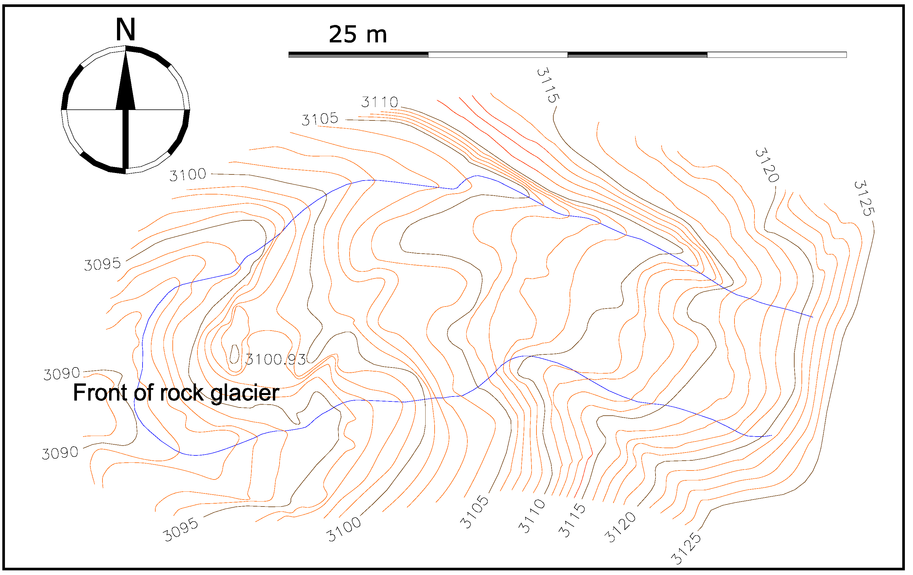
• The map was made from the stereoscopic orientation of the image pair through contour lines with the PRO600 software (Figure 4).

Figure 4. Map of the Veleta rock glacier (scale: 1/1,000, contour lines: 1 m).

Figure 4. Map of the Veleta rock glacier (scale: 1/1,000, contour lines: 1 m).

4. Computer vision for Photogrammetric Reconstruction

The goal of the photogrammetric method presented in this work is to obtain automatically a 3D model of a geomorphologic structure. This method develops preliminary work presented in the Sixth International Conference on Geomorphology [17]. The methodology proposed is supported by means of techniques developed in the field of Computer Vision. The input requirements of the method are: a set of images of the geomorphologic structure taken from different points of view and the camera calibration (focal length, principal point and radial distortion). For the Veleta rock glacier example we work using a digital camera (Canon EOS 5D with 35 mm lens). In this section we present the different method steps which are summarized as follows:

• Extraction features: Extraction of point features of each image using the SIFT extractor [17,18].
• Matching of points (between image pairs).
• Robust matching through the epipolar geometry: The epipolar geometry (a geometric constraint) of the image pair is computed by using robust statistic techniques. Matches that do not hold the epipolar constraint are removed as mismatches.
• Camera processing (pose estimation): We know the internal parameters of camera (focal lenght, principal point, radial distortion) and we estimate the rotation and translation of the cameras.
• DTM generation: This step requires the camera projection matrices and a triangulation process to obtain a 3D model of the geomorphologic structure.

4.1. Extraction of Features

In the first step, feature points are extracted from each image. The more usual image features are points [19], or lines [20]. Here we choose point features because they are more easily extracted in nonstructured environments. We use DoG (Difference of Gaussian) detector and SIFT descriptor to extract a set of point features [18].

The regions extracted with DoG detector are described with a vector of dimension 128 and the descriptor vector is divided by the square root of the sum of the squared components to get illumination invariance. The descriptor is a 3D histogram of gradient location and orientation. SIFT descriptors are very interesting because they are invariant to scale and rotation and have good properties with regard to repeatability, distinctiveness, and robustness, and then, SIFT has shown to be very useful for point matching purposes. For example, we can distinguish the same point in several images even with big scale and orientation changes. In this way we obtain a set of point features for each image of stereo pair using SIFT descriptors, which we use for find pair of corresponding points.

Although there are other descriptors or methods it was demonstrated with different measures that the SIFT descriptors are superior to most others. Several works have compared existing descriptors and concluded that SIFT is a good feature point extractor method in a general use or in photogrammetric applications [21].

4.2. Matching of Points

The SIFT method provides a set of image locations and descriptors. We will use this information for matching points process. We obtain a list of image 1 descriptors and a list of image 2 descriptors that form a database of keypoints. The best candidate for a matching is his closer keypoint neighbor in database, that is to say, the keypoint with lowest euclidean distance respect the correspondent descriptor. Nevertheless, many of the image points do not have an equivalent matching point. Thus, it is necessary a way to remove points whithout a good matching in database.

A priori, the more successful solution is to establish a threshold for the distance to the closer descriptor and even better to compare the distance between the closer neighbour and second closer neighbour. Using this method we remove 90% of wrong matched points and we loose only 5% of correct ones [18]. As we can see in the next sections, SIFT matched points are very good for obtaining an accurate DTM of rock glacier area.

4.3. Robust Matching through the Epipolar Geometry

In this step the epipolar constraint is exploited to remove the wrong matches which still remain. Now, we briefly introduce some concepts related to the epipolar geometry [22] and how it can be used to perform a robust matching [23].

An image taken by a camera is the projection of a 3D scene in a 2D plane. Then, for each 3D point P = (X,Y,Z) we have a projected point in the image plane with coordinates p₁ = (u₁,v₁,1) in the first image and p₂ = (u₂,v₂,1) in the second. The epipolar geometry represents the intrisic geometry between two views. It is independent of the scene structure and only depends on the relative localization between the cameras (rotation and translation) and the internal camera calibration. The baseline is defined as the straight line that joins the optical centers of the cameras. The epipoles (e₁,e₂) are the intersection points of the baseline with the image planes. The fundamental matrix F is the algebraic representation of the epipolar geometry and it satisfies the so called epipolar constraint: p₂^T F p₁ = 0. Therefore, each pair of matched points (p₁,p₂) must hold this constraint; otherwise it is a wrong match.

Each correspondence gives one equation through the epipolar constraint. The fundamental matrix is a 3 × 3 matrix and therefore it can be computed up to scale by solving a linear system from a minimum set of 8 points matches [22]. Nevertheless we must assume that outliers and mismatches are present in the set of point matches. Thus, the fundamental matrix is computed iteratively with the RANSAC method [24], which is robust in presence of outliers. The result of this step is the fundamental matrix relating the pair of images. The point matches that support this fundamental matrix are considered good correspondences and the rest of matches are discarded as wrong matches.

4.4. Camera Processing (Pose Estimation)

We use a previously calibrated camera (focal length, principal point, radial distortion). Therefore if we want to get the complete camera system we need to calculate the exterior orientation (rotation and translation of cameras or camera pose).

Figure 5. Photograph of the distribution of control points (E1–E9) denoted with marks, around the Veleta rock glacier (2008).

Figure 5. Photograph of the distribution of control points (E1–E9) denoted with marks, around the Veleta rock glacier (2008).

We use a nonlinear method to calculate the exterior orientation: The bundle adjustment [25]. The purpose of bundle adjustment is to get an optimization to minimize the reprojection error through a Gradient Descent solution. We calculate an inicialization using DLT (Direct Linear Transform) and use an iterative approximation to minimize reprojection error. In this bundle adjustment process we use a set of control points, that is to say points with known 3D coordinates (Figure 5). Although bundle adjustment could be used to obtain a self-calibration, we only use it for exterior orientation process (pose camera estimation) since we know camera calibration.

4.5. DTM Generation

In this step the 3D reconstruction of the scene is performed to produce the DTM from the set of projection camera matrices. We know the internal camera parameters and the exterior orientation (pose estimation) from the camera processing step in section 4.4, therefore we have now a calibrated system.

As we know the camera projection matrices, the 3D structure may be recovered by triangulation [22]. A simple scheme is proposed using a linear triangulation method to recover the 3D structure [26]. This scheme is based in the fact that the image points have noise and therefore the rays back-projected from the noisy matches in the images are skew in the space. Since the rays do not intersect in general in just one point, the measured points do not satisfy exactly the epipolar constraint. Then, triangulation by back-projecting rays from the matches will fail. This problem is solved if the match points are corrected by minimizing a cost function which represents errors in the image. Once the points are corrected, a linear triangulation method can be carried out to obtain the 3D structure. This 3D structure can be improved using bundle adjustment process as we do for pose estimation. At the end of the triangulation we get a cloud of 3D points. The last step is to convert this 3D point cloud in a surface using a Delaunay triangulation.

5. Results and Discussion

We test the proposed methodology in Veleta rock glacier using 2008 campaign images. As we explain in previous sections we obtained these images using a digital camera, specifically a Canon EOS 5D with a 35 mm lens. We can use the proposed methodology with all the possible pair combinations, but the results are better when we use a pair of camera poses with enough baseline. In order to show the obtained results we follow the steps of our methodology working with a pair of images. We use images 1 and 5 with a baseline of 31.96 m:

• Extraction of features (SIFT). After using SIFT method in images 1 and 5 we get 136,232 keypoints and 94,775 keypoints respectively. As we explain in a previous section these keypoints are invariant to scale, pose, and changes of ilumination.
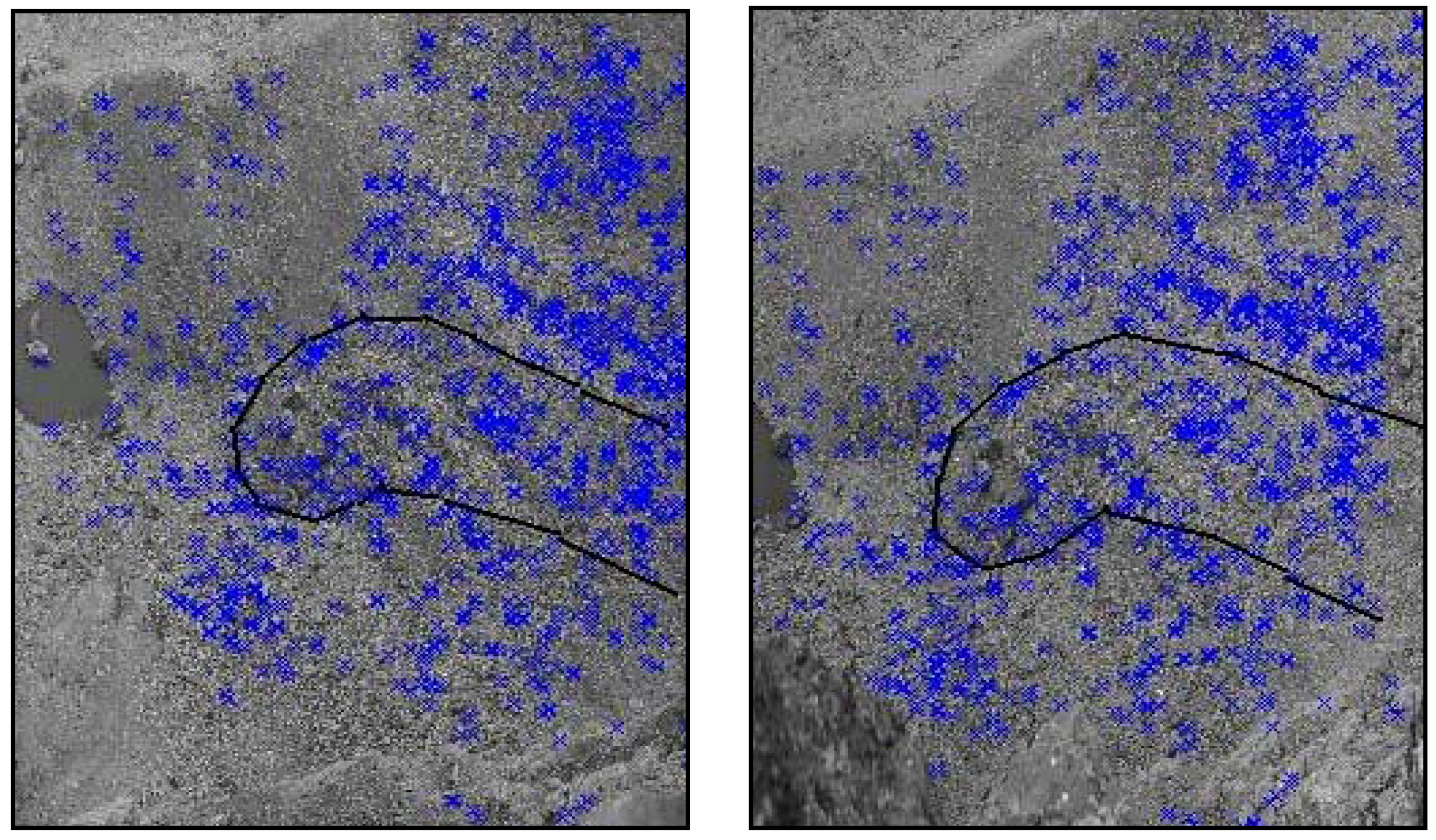
• Matching of points. The next step is the comparison of the two groups of keypoints. In this case we set a threshold of 0.6 for the distance between descriptors and we obtain 17,542 matching locations between image 1 and image 5. Figure 6 represents points (blue crosses) which have a matched point in the other image. Each represented point in left image has an equivalent point in the right image and vice versa.
• Robust matching through epipolar geometry. We use RANSAC method to calculate matrix F with SIFT matching points. The outliers percentage is very low, in this case there are two outliers and 15,540 inliers and a reprojection error average of 0.0594 pixels and a maximum of 3.36 pixels. In this case RANSAC use is not decisive, but it could be important in other examples to get robust matching.

  Figure 6. SIFT matched points denoted with crosses between two images of the Veleta rock glacier area.

  Figure 6. SIFT matched points denoted with crosses between two images of the Veleta rock glacier area.
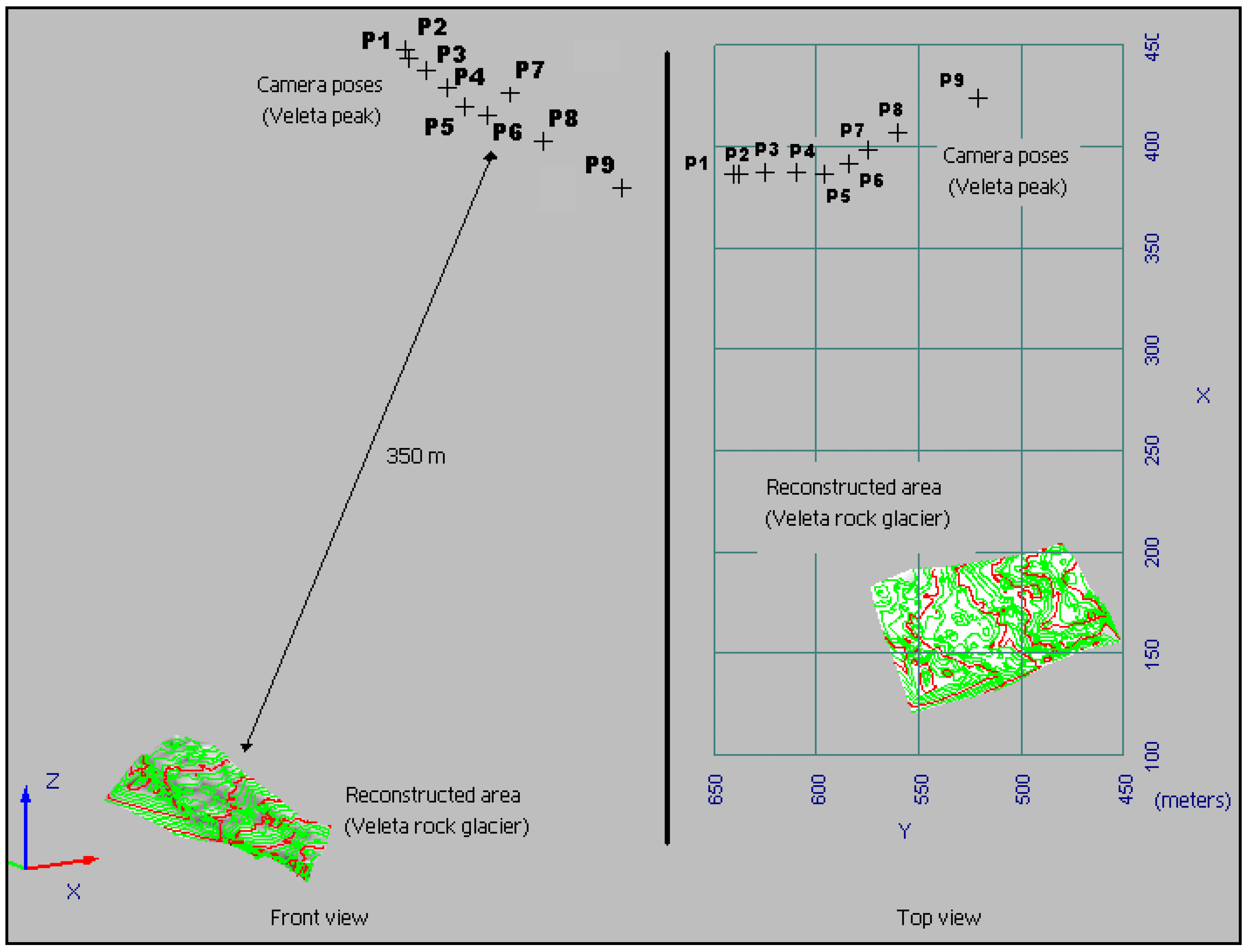
• Camera processing. We show in Table 1 the reprojection error (in the control points E1, E2, ..., E9) obtained computing the cameras (P1, P2, ..., P9) using bundle adjustment method. In Figure 7 we can observe the camera poses respect the rock glacier.

  Figure 7. Camera pose estimation (front view and top view).

  Figure 7. Camera pose estimation (front view and top view).

  Table 1. Camera system accuracy in the year 2008.

  Cameras	Average (in pixels) respect points {E1, …, E9}
  P1	0.69
  P2	0.43
  P3	0.53
  P4	0.38
  P5	0.53
  P6	0.40
  P7	0.45
  P8	0.42
  P9	0.63
  Average all cameras (in pixels)	0.50

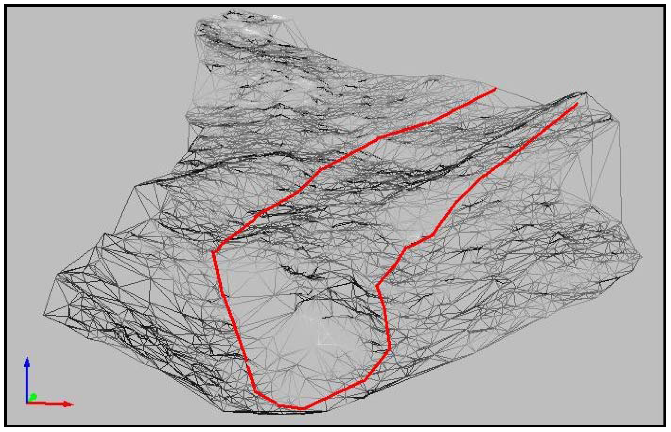
  Table 1. Camera system accuracy in the year 2008.

  Cameras	Average (in pixels) respect points {E1, …, E9}
  P1	0.69
  P2	0.43
  P3	0.53
  P4	0.38
  P5	0.53
  P6	0.40
  P7	0.45
  P8	0.42
  P9	0.63
  Average all cameras (in pixels)	0.50

• DTM generation. Once we know the camera projection matrices we triangulate corresponding points to get a 3D reconstruction. We used the method propose in Section 4.5, getting a reprojection error average of 1.40 pixels and a maximun of 4.50 pixels. Therefore we have 15,540 points (X,Y,Z) of the rock glacier area which we can convert in a surface using a Delaunay triangulation (Figure 8).

Figure 8. Example of Delaunay triangulation of the rock glacier (the view is oriented as in Figure 9).

Figure 8. Example of Delaunay triangulation of the rock glacier (the view is oriented as in Figure 9).

We use cross sections of our reconstructed surface (15,540 points in a Delaunay triangulation surface) to calculate the obtained accuracy. We compare our cross sections with an accurate reconstruction (cross sections obtained using a total station Topcon GTS-502E). As we can see the results are acceptable (errors < 25 cm in height and planimetry) and therefore using this methodology we can get accurate surfaces (Figure 9). We have developed necessary code using Matlab software for method implementation and we have used Photomodeler and Topcon Image Master for internal camera calibration.

Figure 9. Comparison of our reconstructed surface cross sections (black polylines) and total station cross sections (blue polylines) and their situation in a Veleta rock glacier sketch.

Figure 9. Comparison of our reconstructed surface cross sections (black polylines) and total station cross sections (blue polylines) and their situation in a Veleta rock glacier sketch.

6. Conclusions

We propose an automatic technique for rock glacier reconstruction using digital images. A significant amount of work in feature matching techniques has been reported in computer vision in recent years improving old techniques. From the results given by our methodology matching process we can conclude that the set of matches obtained is very good. Using this kind of techniques the post processing cost and time needed to analyze image information of geomorphologic structures can be dramatically reduced avoiding the arduous task of manual photogrammetric restitution.

Usually the images are taken with the same camera but the proposed methodology presents the advantage that it works the same using several types of camera, being each one defined by its own calibration. Thus, the cartography will be automatically produced even if the photographs are taken with different cameras or their external geometry includes variations in orientation or scale. Besides, the non-metric basis of the fundamental matrix used for the robust matching step makes possible to work with different and uncalibrated cameras for obtaining the final set of point matches.

Another advantage of the proposed method is that it deals with convergent images to produce a DTM of rock glaciers. It allows one to work with different types of cameras with acceptable results. The results quality also depends on the camera configuration in the acquisition phase, where large image base pairs with convergent views produce better results.

The presented method offers several advantages for the study of geomorphologic structures in terms of cost and time. Thus, we do not need flights of planes to obtain the photographs. The geodetic data are obtained in short time and we avoid the manual photogrammetric restitution in the office. Using this methodology points are automatically matched between images obtaining that nearly 100% of the matches are correct. Therefore, it is a robust method for the automatic 3D restitution to be used in the production of geomorphologic maps. In order to show the validity of the methodology experiments with different pairs of images of the rock glacier have been performed and the most representative are shown. Future work is focussed toward dense matching and also on extending this method to images taken at different periods of time to study the evolution of the rock glacier. The objective is to have a cheap and fast tool for studying the evolution of the rock glacier along the time, which is our current research goal.

References and Notes

- Sanjosé, J.J.; Atkinson, A.D.J.; Salvador, F.; Gómez, A. Application of geomatic techniques to monitoring of the dynamics and to mapping of the Veleta rock glacier (Sierra Nevada, Spain). Zeitschift für Geomorphologie 2007, 51, 79–89. [Google Scholar] [CrossRef]
- Serrano, E.; Sanjosé, J.J.; Agudo, C. Rock glacier dynamics in a marginal periglacial high mountain environment: Flow, movement (1991–2000) and structure of the Argualas rock glacier, the Pyrenees. Geomorphology 2006, 74, 285–296. [Google Scholar] [CrossRef]
- Sanjosé, J.J.; Lerma, J.L. La fotogrametría digital: Una herramienta idónea para el cartografiado y modelado de zonas de alta montaña. In Congreso de periglaciarismo en montaña; Potes, Spain, 2001; pp. 185–203. [Google Scholar]
- Corripio, J.G. Snow surface albedo estimation using terrestrial photography. Int. J. Remote Sens. 2004, 25, 5705–5729. [Google Scholar] [CrossRef]
- Gómez, A.; Schulte, L.; Salvador, F.; Palacios, D.; Sanjosé, J.J.; Atkinson, A.D.J. Deglaciación reciente de Sierra Nevada. Repercusiones morfogenéticas, nuevos datos y perspectivas de estudio futuro. Cuadernos de investigación geográfica de la Universidad de la Rioja 2004, 30, 147–168. [Google Scholar] [CrossRef]
- Bauer, A.; Paar, G.; Kaufmann, V. Terrestrial laser scanning for rock glacier monitoring. In Proceedings of the 8th International Conference on Permafrost, Zurich, Switzerland; 2003; pp. 55–60. [Google Scholar]
- Kenyi, L.W.; Kaufmann, V. Estimation of rock glacier surface deformation using SAR interferometry data. IEEE TGARS 2003, 41, 1512–1515. [Google Scholar] [CrossRef]
- Roer, I.; Kääb, A.; Dikau, R. Rockglacier acceleration in the Turtmann valley (Swiss Alps): Probable controls. Norwegian J. Geography 2005, 50, 157–163. [Google Scholar] [CrossRef]
- Kääb, A.; Haeberli, W.; Gudmundsson, G.H. Analysing the creep of mountain permafrost using high precision aerial photogrammetry. 25 years of monitoring Gruben rock glacier. Swiss Alps. Permafrost Periglac. 1997, 8, 409–426. [Google Scholar] [CrossRef]
- Kääb, A.; Kneisel, C. Permafrost creep within a recently deglaciated glacier forefield: Muragl, Swiss Alps. Permafrost Periglac. 2006, 17, 79–85. [Google Scholar] [CrossRef]
- Kaufmann, V.; Ploesch, H. Mapping and visualization of the retreat of two cirque glaciers in the Austrian Hohe Tauern National Park. In XIX ISPRS Congress International Archives of Photogrammetry and Remote Sensing, Amsterdam, The Nederlands, July 16–22, 2000; 2000; Volume XXXIII, Part B4. pp. 446–453. [Google Scholar]
- Kaufmann, V.; Ladstädter, R.; Kienast, G. 10 Years of monitoring of the Doesen rock glacier (Ankogel group, Austria)—A review of the research activities for the time period 1995–2005. In 5th ICA Mountain Cartography Workshop, Bohinj, Slovenia, March 30–April 1, 2006; pp. 129–144.
- Sanjosé, J.J.; Lerma, J.L. Estimation of the rocks glaciers dynamics by environmental modeling and automatic photogrammetric technic. In XX Congress International Society for Photogrammetry and Remote Sensing, Commission VII, Istanbul, Turkey, July 12–23, 2004; Vol. XXXV-B7.
- Gómez, A.; Palacios, D.; Ramos, M.; Casas, A.; Sanjosé, J.J.; Atkinson, A.D.J. Permafrost, evolución de formas asociadas y comportamiento térmico en el corral del Veleta (Sierra Nevada, España), Últimos resultados. Boletín de la Real Sociedad Española de Historia Natural (Sección Geológica) 2004, 99, 47–63. [Google Scholar]
- Mikhail, E.M.; Bethel, J.S.; McGlone, J.C. Introduction to Modern Photogrammetry; John Wiley: NY, USA, 2001. [Google Scholar]
- Wolf, P.R.; Dewitt, B.A. Elements of Photogrammetry with aplications in GIS; McGraw Hill: Boston, MA, USA, 2000. [Google Scholar]
- López-Nicolás, G.; Guerrero, J.J.; Sanjosé, J.J. Automatic photogrammetry for the production of geomorphologic cartography. In Sixth International Conference on Geomorphology, Zaragoza, Spain, September 7–11, 2005.
- Lowe, D. Distinctive Image Features from Scale-Invariant Features. Int. J. Comput. Vision 2004, 60, 91–110. [Google Scholar] [CrossRef]
- Zhang, Z.; Deriche, R.; Faugeras, O.; Luong, Q.T. A robust technique for matching two uncalibrated images through the recovery of the unknown epipolar geometry. Artificial Intelligence 1995, 78, 87–119. [Google Scholar] [CrossRef]
- Guerrero, J.J.; Sagüés, C. Robust line matching and estimate of homographies simultaneously. In Iberian Conference on Pattern Recognition and Image Analysis, 2652 Lecture Notes in Computer Science, Mallorca, Spain, June 4–6, 2003; pp. 297–307.
- Remodino, F. Detectors and descriptors for photogrammetric applications. In Photogrammetry and Computer Vision, Bonn, Germany, September 20–22, 2006.
- Hartley, R.; Zisserman, A. Multiple View Geometry in Computer Vision, 2nd ed.; Cambridge University Press: NY, USA, 2004. [Google Scholar]
- Rousseeuw, P.; Leroy, A. Robust regression and outlier detection; John Wiley: New York, NY, USA, 1987. [Google Scholar]
- Fischler, M.A.; Bolles, R.C. Random sample consensus: A paradigm for model fitting with applications to image analysis and automated cartography. Commun. Assn. Comput. Mach. 1981, 24, 381–395. [Google Scholar] [CrossRef]
- Triggs, B.; McLauchlan, P.; Hartley, R.; Fitzgibbon, A. Bundle adjustment – A modern synthesis. In Proceeding International ICCV Workshop on Vision Algorithms, Corfu, Greece, September 21–22, 1999; Springer: Berlin/Heidelberg, Germany, 2000; 1883, pp. 298–372. [Google Scholar]
- Torr, P.H.S. A Structure and Motion Toolkit in Matlab; Technical Report MSR-TR-2002-56; Microsoft Research: Cambridge, UK, 2002. [Google Scholar]
© 2009 by the authors; licensee Molecular Diversity Preservation International, Basel, Switzerland. This article is an open-access article distributed under the terms and conditions of the Creative Commons Attribution license ( http://creativecommons.org/licenses/by/3.0/).
Share and Cite
De Matías, J.; De Sanjosé, J.J.; López-Nicolás, G.; Sagüés, C.; Guerrero, J.J. Photogrammetric Methodology for the Production of Geomorphologic Maps: Application to the Veleta Rock Glacier (Sierra Nevada, Granada, Spain). Remote Sens. 2009, 1, 829-841. https://doi.org/10.3390/rs1040829
De Matías J, De Sanjosé JJ, López-Nicolás G, Sagüés C, Guerrero JJ. Photogrammetric Methodology for the Production of Geomorphologic Maps: Application to the Veleta Rock Glacier (Sierra Nevada, Granada, Spain). Remote Sensing. 2009; 1(4):829-841. https://doi.org/10.3390/rs1040829
Chicago/Turabian StyleDe Matías, Javier, José Juan De Sanjosé, Gonzalo López-Nicolás, Carlos Sagüés, and José Jesús Guerrero. 2009. "Photogrammetric Methodology for the Production of Geomorphologic Maps: Application to the Veleta Rock Glacier (Sierra Nevada, Granada, Spain)" Remote Sensing 1, no. 4: 829-841. https://doi.org/10.3390/rs1040829
APA StyleDe Matías, J., De Sanjosé, J. J., López-Nicolás, G., Sagüés, C., & Guerrero, J. J. (2009). Photogrammetric Methodology for the Production of Geomorphologic Maps: Application to the Veleta Rock Glacier (Sierra Nevada, Granada, Spain). Remote Sensing, 1(4), 829-841. https://doi.org/10.3390/rs1040829