Hyperspectral Shallow-Water Remote Sensing with an Enhanced Benthic Classifier

Abstract

Hyperspectral remote sensing inversion models utilize spectral information over optically shallow waters to retrieve optical properties of the water column, bottom depth and reflectance, with the latter used in benthic classification. Accuracy of these retrievals is dependent on the spectral endmember(s) used to model the bottom reflectance during the inversion. Without prior knowledge of these endmember(s) current approaches must iterate through a list of endmember—a computationally demanding task. To address this, a novel lookup table classification approach termed HOPE-LUT was developed for selecting the likely benthic endmembers of any hyperspectral image pixel. HOPE-LUT classifies a pixel as sand, mixture or non-sand, then the latter two are resolved into the three most likely classes. Optimization subsequently selects the class (out of the three) that generated the best fit to the remote sensing reflectance. For a coral reef case, modeling results indicate very high benthic classification accuracy (>90%) for depths less than 4 m of common coral reef benthos. These accuracies decrease substantially with increasing depth due to the loss of bottom information, especially the spectral signatures. We applied this technique to hyperspectral airborne imagery of Heron Reef, Great Barrier Reef and generated benthic habitat maps with higher classification accuracy compared to standard inversion models.

1. Introduction

Although coral reef and other coastal ecosystems provide high socio-economic benefits, they continue to decline due to global impacts such as heightened thermal stress and ocean acidification, as well as from local human induced impacts of over-fishing, destructive fishing, coastal development, influx of pollution, and spread of marine diseases and invasive species [1,2,3]. Promoting coral reef resilience and adaptability requires effective management strategies [3], which in turn are aided by large-scale habitat maps that remote sensing can produce [4,5]. The ability to operationally reproduce high accuracy maps over large spatial areas (>1000 km²) is therefore paramount, as it can directly influence the effectiveness of management strategies [6,7].

A primary goal for remote sensing in coral reefs where the water-leaving signal is dominated by the bottom (i.e., optically shallow water), is the derivation of bottom reflectance that can be subsequently used in benthic classification. Unfortunately, the benthic signal is reduced by the depth and the absorptive and scattering properties of the overlying water column that synergistically determine the above-water remote sensing reflectance, R_rs [8]—an apparent optical property that can be derived from passive remote sensing platforms. Under such optically complex conditions, approaches that can differentiate the impact of the water column from that of the bottom reflectance solely from R_rs are desired. Indeed, research into the benthic classification from multispectral imagery has indicated that higher classification accuracies are obtained from approaches that remove the influences of the water column [9,10].

Physics-based semi-analytical (SA) inversion algorithms and look up table (LUT) approaches are two such methodologies that can achieve this. Both SA and LUT methods rely on matching between the sensor-derived and modeled R_rs spectra [11]. These have been primarily developed for hyperspectral sensors, where the number of bands in the visible domain (with a high enough signal-to-noise ratio) can detect subtle spectral differences in the water-leaving radiance due to changes in depth, bottom substrate or magnitudes of in-water optically active constituents [12]. The high amount of spectral information afforded by hyperspectral imagery theoretically minimizes non-uniqueness issues in the retrieved water inherent optical properties (IOPs), bottom depth and bottom reflectance, hence reducing uncertainty [13,14].

The past two decades have seen the development of several SA models; however all can be traced back to Hyperspectral Optimization Processing Exemplar (HOPE; Lee et al. [15]), which employs semi-analytical expressions to approximate the radiative transfer equation, relating R_rs to the IOPs, depth and bottom reflectance. Additionally, parameterizations of the water column’s absorption and backscattering coefficients and bottom reflectance are made such that each can be represented by a scalar variable. Spectral optimization is then applied to determine the values of the scalar variables whose modeled R_rs ($R_{\mathrm{rs}}^{\mathrm{M}}$) best matches the sensor-derived R_rs ($R_{\mathrm{rs}}^{\mathrm{sens}}$). SA models based on Lee et al. [15] include BRUCE [16], SAMBUCA [17] and BOMBER [18] and those described in Jay et al. [19] and Petit et al. [20]. However, use of a single endmember to model bottom reflectance (as in HOPE) confounds benthic retrievals for heterogeneous pixels or other pixels not represented by the single endmember.

LUT methodologies such as CRISTAL [14] and ALLUT [21] search for the $R_{\mathrm{rs}}^{\mathrm{M}}$ spectrum within a large dataset (the LUT) that best matches the $R_{\mathrm{rs}}^{\mathrm{sens}}$. The corresponding IOPs, depth and benthic substrate (assuming spatially uniform substrate for a given pixel) are then assumed to match the conditions that formed the $R_{\mathrm{rs}}^{\mathrm{sens}}$. The differences between CRISTAL and ALLUT lie in the selection of the model parameters (depth, IOPs, bottom reflectance), the searching algorithm and the minimization of the resultant discretization errors. In an intercomparison between a variety of LUT and SA methodologies, Dekker et al. [11] showed that BRUCE obtained the highest overall benthic classification accuracy of 79% followed by ALLUT (78%), CRISTAL (65%) and SAMBUCA (52%). Thus, SA and LUT methodologies can be comparable. For SA models the benthic classification accuracy is dependent on the suitability of the assumptions to the radiative transfer equation, where the total absorption and backscattering coefficients are decomposed into a limited set of optically active constituents. In contrast, the accuracy of LUT methods is dependent on the minimization of discretization errors and whether the finite IOPs, depth and bottom substrate combinations included in the LUT are representative of the imaged area. Both SA and LUT methods must define the benthic endmembers and spectral shapes of the IOPs beforehand.

A key input to any SA inversion model is the spectral shape of the bottom reflectance (ρ) to invert the corresponding R_rs of a given pixel. Paradoxically, ρ is unknown prior to any processing, and, even more problematically, the use of an incorrect ρ can lead to inaccurate retrievals of IOPs and depth. In the standard application of the HOPE inversion algorithm [15,22], ρ was chosen to be that of a single “pure” endmember of Sand or Seagrass based on scene-specific reflectance and reflectance-ratio values. As such, HOPE is more applicable to very high spatial resolution imagery or over spatially homogeneous regions where a pixel is dominated by a single benthic class. In the BRUCE [16] and SAMBUCA [17] inversion models, ρ is modeled as a linear mixture of three and two benthic endmembers, respectively. Given that a coral reef environment has more than three (or two) benthic components, a common practice is to iterate through unique combinations of endmembers in a benthic spectral library during the inversion. This allows for the modeling of multiple sets of benthic endmembers (e.g., Sand/Brown Algae/Coral, Sand/Turf Algae/Seagrass etc.). By doing so, these inversion models optimize for the IOPs (or as in the case of SAMBUCA, the concentrations of optically active water constituents), depth and a “refined” (albeit modeled) ρ. This is a computationally expensive procedure requiring multiple inversions per-pixel to find the benthic endmember combination that yields the lowest relative error between the $R_{\mathrm{rs}}^{\mathrm{M}}$ and $R_{\mathrm{rs}}^{\mathrm{sens}}$. For example, using a three component model (e.g., BRUCE), a library of seven benthic endmembers would result in 35 unique combinations, i.e., 35 inversions per pixel. A two component model (e.g., SAMBUCA) in this case would result in 21 inversions per pixel. Note that, for each inversion, the optimization algorithm would require usually tens of iterations to minimize the cost function.

In this paper, we develop an LUT-based approach that preselects the likely benthic classes from an R_rs spectrum and an initial estimate of the depth, thereby significantly narrowing the selection of potential benthic endmembers from a spectral library. These selected endmembers can then be applied in an inversion model to retrieve the IOPs, depth and a refined ρ more efficiently than currently employed schemes (e.g., BRUCE or SAMBUCA). At the same time, the new approach overcomes the caveats of the default HOPE model (single endmember) that cannot handle subpixel benthic variations (spectral mixing). The LUT-based approach splits the database of $R_{\mathrm{rs}}^{\mathrm{M}}$ into smaller fragments (termed nodes) from which a classifier is generated. Self-consistency tests indicate that these classifiers are robust against the spectral variability present within each benthic endmember. We have implemented this approach to hyperspectral airborne PRISM (Portable Remote Imaging Spectrometer) imagery of Heron Reef, Great Barrier Reef, Australia. The benthic classification map generated for Heron Reef is consistent with that previously published [6,23] and obtains higher classification accuracy than the map generated by the standard BRUCE model. HOPE-LUT represents a standardized approach of preselecting benthic endmembers used in benthic classification, without the use of scene-specific training datasets as in traditional supervised classification, to simultaneously retrieve IOPs, bottom depth and reflectance.

2. Materials and Methods

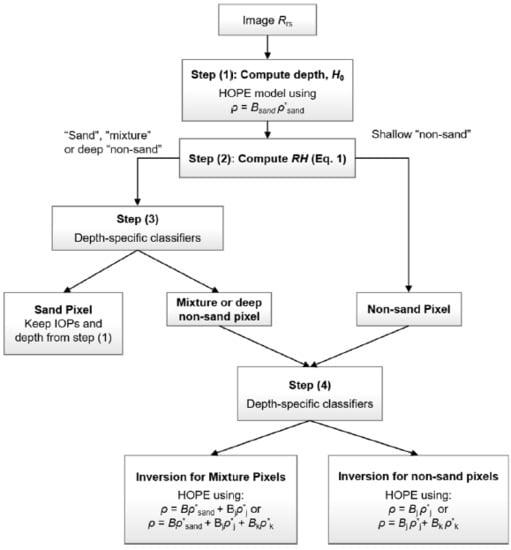
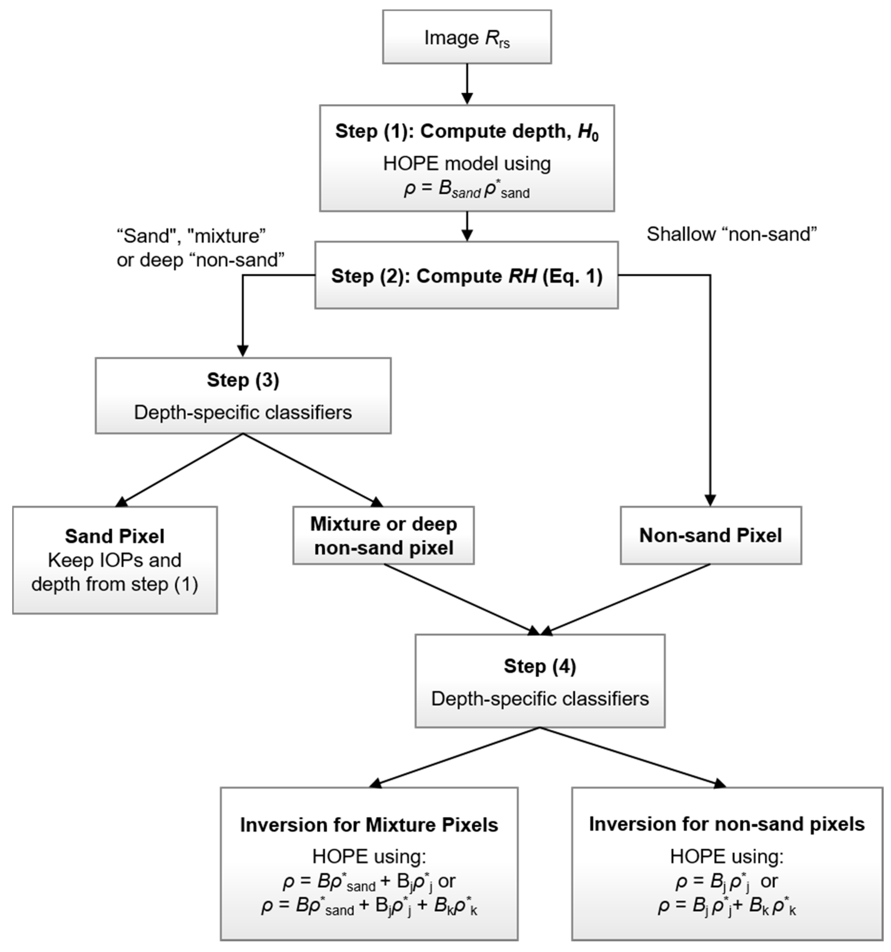
We present a four-stage workflow (Section 2.1) for the preselection of the benthic endmembers that are input to a shallow water inversion model for the retrieval of IOPs and depth. The classification approach utilizes classifiers generated from an LUT of modeled R_rs (

Table 1. The relevant acronyms and symbols and their definitions.

Acronym	Units	Definition
IOPs		Inherent Optical Properties
SA		Semianalytical model
LUT		Look up table
BSP		Binary Space Partitioning
PCA		Principal Component Analysis
HOPE		Hyperspectral Optimization Process Exemplar
BRUCE		Bottom Reflectance Un-mixing Computation of the Environment
PRISM		Portable Remote Imaging Spectrometer
rrs	sr−1	Subsurface remote sensing reflectance
Rrs	sr−1	Above-water remote sensing reflectnace
$R_{\mathrm{r}\mathrm{s}}^{\mathrm{M}}$	sr−1	Forward modeled Rrs
$R_{\mathrm{rs}}^{\mathrm{sens}}$	sr−1	Sensor-derived Rrs
ρi(λ)	dimensionlesss	Bottom reflectance of class i
${\rho }_{\mathrm{i}}^{*}$(λ)	dimensionlesss	ρi(λ) normalized to a value of 1.0 at 550 nm
${Pr}_{\mathrm{rs}}^{\mathrm{B}}$	dimensionless	Percentage contribution of the bottom signal to rrs
Λ	nanometers	Wavelength
θs	radians	Solar zenith angle
aw(λ)	m−1	Absorption coefficient of pure water
aphy(λ)	m−1	Absorption coefficient of phytoplankton
adg(λ)	m−1	Absorption coefficient of detritus and gelbstoff
bbw(λ)	m−1	Backscattering coefficient fo pure water
bbp(λ)	m−1	Backscattering coefficient of suspended particles
P	m−1	aphy(440)
G	m−1	adg(440)
X	m−1	bbp(440)
H	m	Geometric depth of the water column
τ	m	Optical depth of the water column
Bi	dimensionless	ρi(550)
RH	sr−1	The relative height of the Rrs peak between 685 and 740 nm

presents a list of relevant symbols and acronyms). Section 2.2.1 and Section 2.2.2 describes the generation of the LUTs and the use of Binary Space Partitioning (BSP) to aid the classification. Section 2.3 describes the shallow water inversion models, while a description of PRISM imagery is provided in Section 2.5.

2.1. Workflow

The approach (Figure 1) begins with step (1), which estimates the depth, H₀, of all optically shallow water pixels using an initial HOPE inversion. H₀ is used in step (3) to aid the distinction between “sand” and “mixture” pixels and in step (4) to select the three most likely benthic classes. We define “mixture” and “non-sand” based on the proportion of Sand present, with “non-sand” as having none to a small proportion of Sand. These shallow “non-sand” pixels were distinguished in step (2), using the relative height, RH, of the R_rs peak between 685 and 740 nm derived from PRISM imagery. This peak is prominent for pixels that are very shallow consisting of non-sand benthos and corresponds to their characteristic high reflectance towards the NIR. This peak is also predominant in pixels that have minor amounts of Sand, hence the reason why “non-sand” was defined as having none to small proportions of Sand.

$$\begin{gathered} RH=R_{\mathrm{rs},\mathrm{peak}}-R_{\mathrm{rs},\mathrm{peak}}^{\prime }, “\mathrm{non-sand}” \mathrm{if} RH>0.003 s{r}^{-1}, \\ {R}_{\mathrm{rs},\mathrm{peak}}^{\prime }= R_{\mathrm{rs},740}+\left(R_{\mathrm{rs},685}-R_{\mathrm{rs},740}\right)\times \left(\frac{{\lambda }_{\mathrm{peak}}-{\lambda }_{740}}{{\lambda }_{685}-{\lambda }_{740}}\right) \end{gathered}$$

(1)

where $R_{\mathrm{rs},\mathrm{peak}}^{\prime }$ and λ_peak are the R_rs value and wavelength of the peak (if any) between 685 and 740 nm, respectively. $R_{\mathrm{rs},\mathrm{peak}}^{\prime }$ is the estimated baseline at this peak, and RH the relative height. Equation (1) follows the form of the MERIS MCI [24] and Floating Algae Index [25] equations, which utilize a spectral peak at the red-edge to identify and quantify floating plant matter. In clear water, shallow (<2 m) Sand displays a similar peak, and a threshold of RH = 0.003 sr⁻¹ sufficiently distinguishes “sand” from “non-sand” in PRISM imagery of Heron Reef. The wavelength of this peak, λ_peak, is not fixed as the absorption caused by an increasingly deep water column shifts the peak’s center towards 680 nm while at the same time decreasing its magnitude. The RH threshold is derived from PRISM imagery, and analysis indicates that a value in the range 0.001–0.004 sr⁻¹ can be used to identify shallow “non-sand” pixels. At the lower end of this range, more “mixture” pixels are identified as “non-sand.” Note that “non-sand” pixels with a retrieved depth >3 m generally had an RH < 0.003 sr⁻¹ for the PRISM image of Heron Reef. Hence a threshold of 0.003 sr⁻¹ is only suitable to identify shallow “non-sand” pixels.

In step (3), a classifier was used to distinguish those pixels whose RH ≤ 0.003 sr⁻¹ as either “sand” or “mixture”/“non-sand.” The latter represents a pixel that could be either “mixture” or “non-sand.” Here, H₀ was used to assign the R_rs to the appropriate depth-specific classifier (see Section 2.2.2) that was trained with a depth range that encompassed H₀. In this study, we generated six depth-specific classifiers for the depth ranges of 0.2–2 m, 2–4 m, 4–6 m, 6–8 m, 8–10 m and 10–12 m. Hence if H₀ = 1.3 m, then the 0.2–2 m classifier was used to assign R_rs as “sand”, “mixture/non-sand.” The rational for using depth-specific classifiers was simply to improve the classification accuracy by reducing the within-class variability and hence inter-class overlap compared to using classifiers trained from an LUT whose modeled depth ranged from 0.2–12 m. Indeed, Hedley et al. [26], showed that variance in depth increases across-depth confusion between classes thereby reducing the separability of the benthic classes. In fact, the reduction in the separability of benthic classes due to variance in depth overwhelms the reduction in separability due to variance in IOPs, sun elevation or sensor signal-to-noise ratio [26].

In step (4), depth-specific classifiers resolved “mixture” and “non-sand” pixels into seven classes consisting of Seagrass, Brown Algae, Calcareous Algae, Turf Algae, Brown Coral and the non-sand mixtures of Brown/Blue Coral and Turf Algae/Brown Coral (see Figure 2b–h). Here, Calcareous Algae refers to crustose coralline algae. Note that (1) Green algae is not included in the classifier because it is unlikely to dominate an 8 × 8 m pixel and can be optically inseparable from seagrass at depth as noted by Garcia et al. [27] (2) Soft coral has also excluded due its spectral similarity with Brown Coral [28] and (3) reflectance spectra for Rubble was not available and thus not included, though it is ecologically important in a coral reef ecosystem. Hochberg et al. [28] describes the spectral features present in Figure 2. The three most likely classes (out of the seven) were then passed to an inversion step that selected the class (out of the three) that generated the best matching $R_{\mathrm{r}\mathrm{s}}^{\mathrm{M}}$ to $R_{\mathrm{rs}}^{\mathrm{sens}}$. A variant of the HOPE model was used in this inversion step, such that the bottom reflectance for “mixtures” was modeled with either two or three components depending if non-sand mixtures (i.e., Brown/Blue Coral or Turf Algae/Brown Coral) were selected. Here one of the bottom components were set as Sand. For “non-sand” pixels the bottom reflectance was modeled either with a single or two bottom components depending if a non-sand mixture was chosen. Section 2.3 discusses these inversions in more detail.

The seven classes used in this study were chosen based on spectral separabilty [28] and ecological importance. In coral reef ecosystems, corals are the fundamental species that provide structural habitat and significantly contribute to reef development and growth rates [29,30]. With regards to reflectance, hard corals exhibit two modes [28,31]; (1) the Brown Coral mode, which has a triple peak pattern with peaks near 575, 600 and 650 nm (Figure 2f), and is exhibited by corals that appear by eye as brown, red, green, orange and green, and (2) the Blue Coral mode, which has a broad plateau-like peak between 600 and 650 nm (see Hochberg et al. [31]). This mode is exhibited by corals that appear pink, gray, purple and blue [28]. Turf Algae and Calcareous Algae dominate coverage on the reef flats and crests [32,33] and hence dominate the net primary production in these areas [34]. Turf Algae are a major food source by primary consumers [35,36], while Calcareous Algae (crustose coralline algae) precipitate calcium carbonate [37] and causes the cementation of the reef pavement which sustains the reef structure [38,39]. Additionally, Calcareous Algae is a preferred substrate for the settlement of certain coral larvae [40]. Macroalgae are a preferred food source for herbivorous fish and echinoids and compete with scleractinian corals for space [41]. Seagrass, although not present in Heron Reef, can occur in the back-reef or lagoon and provides habitat and predation refuge to a diverse range of fauna [42].

2.2. Depth-Specific Classifiers

2.2.1. LUT Generation

Depth-specific classifiers were generated from a LUT of modeled R_rs. We follow the approach of ALLUT [21] where the forward model given by [15,22] was used for the efficient generation of large datasets of R_rs (>4.0 × 10⁶ spectra, 400–700 nm, 3 nm resolution) that encompass a wide range of IOPs (Equation (2)), depth and bottom reflectance.

0.003 ≤ a_phy(440) ≤ 0.2 m⁻¹
0.001 ≤ a_dg(440) ≤ 0.6 m⁻¹
0.001 ≤ b_bp(440) ≤ 0.01 m⁻¹

(2)

a_phy(440) of 0.17 m⁻¹ approximately equals a chlorophyll-a concentration of 5 mg m⁻³ [43] and was included in case optically complex water were encountered. Bottom reflectance was parameterized using the spectral library presented in [28] that included the spectral variability of Sand, Seagrass, Brown Algae, Calcareous Algae (crustose coralline algae), Turf Algae and Brown and Blue Corals. To reduce discretization errors in the resultant LUT, we applied an iterative subdivision approach, analogous to Hedley et al. [21], to the depth parameter. Thus, for a given IOP combination and ρ the depth was sampled to generate uniform sampling at R_rs(550). Although the IOPs were sampled evenly in parameter space, the resultant discretization errors would be less of an issue as classifiers were created rather than using the LUT for spectral matching. Furthermore, $R_{\mathrm{r}\mathrm{s}}^{\mathrm{M}}$ with weak bottom reflectance signal were excluded from the LUT by excluding $R_{\mathrm{r}\mathrm{s}}^{\mathrm{M}}$ whose bottom contribution to R_rs (notated as ${Pr}_{\mathrm{rs}}^{\mathrm{B}}$) was less than 30% at the most water penetrating wavelength.

For the sand/mixture depth-specific classifiers in step (3), six LUTs were generated with modeled depths of 0.2–2 m, 2–4 m, 4–6 m, 8–10 m and 10–12 m. We limit the depth to 12 m as shallow water inversion models typically struggle to retrieve accurate depths beyond this depth (e.g., [11]). We also included a 20% variability in the bounding depth; for instance, the 2–4 m LUT included depths that ranged from 1.6 m to 4.8 m. This was to account for possible errors in the initial depth, H₀, which was used to assign the input R_rs to the appropriate depth-specific classifier. For these LUTs, the depth parameter was iteratively subdivided 13 times between the depth bounds and the IOPs were sampled at 30 regular intervals between the IOP bounds specified in Equation (2). The bottom reflectance of seven Sand and seven representative mixtures were used to model the R_rs. The latter seven ρ mixtures were generated in the following manner: (a) 77 combinations of 70%/30% sand/non-sand mixture ρ were created from seven Sand and eleven non-sand ρ, and; (b) N-FINDR endmember extraction [44] was run 1000 times and the seven most occurring endmembers were selected to represent the mixture class in the LUT. Here, the non-sand ρ taken from Hochberg et al. [28] were terrigenous mud, Bleached Coral, Brown Macroalgae, Green Algae, Red Algae, Calcareous Algae, Turf Algae, Blue Coral, Brown Coral, Soft/Gorgonian Coral and Seagrass.

For the non-sand classifiers in step (4), six LUTs were generated using the same depth ranges as listed above, with a 20% variability included in the bounding depths. Here the depth parameter was subdivided 10 times between the depth bounds and the IOPs were sampled at 15 regular intervals between the IOP bounds specified in Equation (2). The LUT at each depth range were generated in the following manner: (a) intra-class variability in the bottom reflectance were included by utilizing more than one spectral shape for the seven classes of Seagrass, Brown Algae, Calcareous Algae, Turf Algae, Brown Coral, Brown/Blue Coral and Turf Algae/Brown Coral (See Figure 2b–h), and; (b) the modeled R_rs were normalized to emphasize classification based on the spectral shape, in order to minimize possible issues with under/over correction during the atmospheric correction.

2.2.2. Classifiers aided by Binary Space Partitioning Trees

Creating benthic classifiers directly from the LUT would reduce their classification accuracy due to the large intra-class variability and inter-class overlap present in the R_rs. A method that reduces this variability in the LUT is therefore crucial. Binary space partitioning (BSP) has been used by Hedley et al. [21] to subdivide a LUT into smaller subsets (termed nodes) for the purpose of efficiently matching $R_{\mathrm{rs}}^{\mathrm{sens}}$ with a R_rs in the LUT. The subdivision produces nodes with lower intra-class variability and would create classifiers with improved accuracy. In the first layer, the BSP subdivides the initial LUT into a left and right child node. Subsequent child nodes are then recursively subdivided into two nodes. This generates a tree-like structure with terminal nodes prior to and at the user-specified tree layer. This tree structure allows an input $R_{\mathrm{rs}}^{\mathrm{sens}}$ to traverse the tree to a terminal node where it is identified as belonging to a benthic class. The creation of the BSP tree is similar to [21], except with minor modifications as described below:

• A principal component analysis (PCA) is performed on the initial LUT of $R_{\mathrm{r}\mathrm{s}}^{\mathrm{M}}$;
• The LUT is subdivided into a left and right child node using a dividing plane in spectral space. This dividing plane is perpendicular to the first principal component and passes through the spectral mean of the LUT;
• The left and right child nodes are then subdivided into two nodes with same procedure, with PCA performed on the given node, thus computing the dividing plane.
• Terminal nodes are formed when a child node contains $R_{\mathrm{r}\mathrm{s}}^{\mathrm{M}}$ from one benthic class or when a benthic class has a lower limit of 50 $R_{\mathrm{r}\mathrm{s}}^{\mathrm{M}}$ spectra. This lower limit is necessary in order to have enough spectra per class to generate a classifier (i.e., a non-singular covariance matrix).
• At each terminal node a classifier is trained from the $R_{\mathrm{r}\mathrm{s}}^{\mathrm{M}}$ spectra present in that node. Additionally, for the classifiers in step (3) of the workflow, 70% of the $R_{\mathrm{r}\mathrm{s}}^{\mathrm{M}}$ of each class present in the node were randomly selected and used to generate the classifier. The remaining 30% were used to assess the misclassification rates. The reasoning behind this is described below.

The dividing plane at each parent node is stored, allowing an input R_rs spectrum to traverse the tree to a terminal node. There, a classifier assigns the input R_rs to a benthic class that exists in that terminal node. The Mahalanobis distance (assuming unequal covariance matrices between classes) is used as the classifier-based its underpinning of quadratic discriminant analysis [45]. To make the classifier robust to spectral noise present in an image R_rs, a PCA-based dimension reduction is performed on all $R_{\mathrm{r}\mathrm{s}}^{\mathrm{M}}$ present in a terminal node. Specifically, all n-band $R_{\mathrm{r}\mathrm{s}}^{\mathrm{M}}$ are converted to s-band spectra, where s is the number of principal components that explained 99.5% of the variance in the terminal node (s < n). The resultant s-band spectra are then used to compute the mean and inverse covariance matrix from each benthic class. Hence, when an input R_rs reaches a terminal node, it is converted to an s-band spectrum and then assigned a benthic classed based on the lowest Mahalanobis distance.

Serious repercussions are encountered if a mixture pixel is misclassified as “sand” in step (3) of the workflow, because there is no possibility to reassign it as “mixture.” The consequences are less severe for sand pixels that are misclassed as “mixture”, as subsequent inversions utilize a sand component in the modeling of the bottom reflectance (see Section 2.3). Hence, for these depth-specific classifiers in step (3), terminal nodes that have a misclassification rate greater than 30% are flagged. If an input R_rs reaches one of these terminal nodes an additional inversion is performed to assess the proportional brightness of the Sand component, P_s. If P_s > 90% then the R_rs is assigned as “sand” and “mixture” if P_s ≤ 90%. Analyzes have shown that P_s never reaches 100%, even over shallow Sand targets. The likely cause of this is the presence of benthic microalgae, which generally have spectral features associated with photosynethic and photo-protective pigments [46]—features that not predominant in the Sand reflectance spectra (Figure 2a) used. Thus, sand pixels with higher concentration of microalgae will have P_s < 100%.

2.3. Retrievals of IOPs and Depth

In the workflow, three variants of the HOPE inversion model are implemented to retrieve IOPs and depth. These variants differ in the way that bottom reflectance, ρ, is modeled. Briefly, the HOPE model approximates r_rs as a function of the absorption coefficients of phytoplankton, P, and of dissolved and detrital matter, G at 440 nm; the backscattering coefficient of suspended particles at 440 nm, X; depth, H; and ρ. Here, P changes the magnitude and shape of the spectral absorption of phytoplankton [11,15,22]. For the inversions, spectral slopes of G and X are set to −0.015 nm⁻¹ and 0.5, respectively, and the spectral optimization approach modified from Garcia et al. [47] is used to obtain more global solutions (see Section 2.3.2).

2.3.1. Parameterization of Bottom Reflectance

For the computation of the initial depth H₀ in step (1), the bottom reflectance is modeled as,

$${\rho }_{\mathrm{Sand}}=B_{\mathrm{Sand}}{\rho }_{\mathrm{Sand}}^{*}$$

(3)

where ρ* is the bottom reflectance normalized to 1.0 at 550 nm, and B represents the retrieved albedo at 550 nm. Although ρ_Sand is not an adequate representation of the bottom reflectance of “mixture” or “non-sand” pixels, it is sufficient to estimate H (e.g., [11,48]). For those R_rs that reach a terminal node and have a misclassification rate ≥30% (in step (3) of the workflow), an additional inversion was used to compute P_s. Here, the bottom reflectance is modeled as,

$$\rho =B_{\mathrm{Sand}}{\rho }_{\mathrm{Sand}}^{*}+B_{\mathrm{mix}}{\rho }_{\mathrm{mix}}^{*}$$

(4)

and P_s as,

$$P_{\mathrm{s}}=\frac{B_{\mathrm{Sand}}}{B_{\mathrm{Sand}}+B_{\mathrm{mix}}}$$

(5)

where ${\rho }_{\mathrm{mix}}^{*}$ is the average ρ^* of Turf Algae and Brown Coral. In this case, B_Sand and B_mix are functions of both the bottom albedo at 550 nm and the fractional coverage of each bottom component [49]. The classes assigned to a “non-sand” pixel in step (4) determined how the bottom reflectance was modeled in the subsequent inversion. There are seven possible classes consisting of five pure endmembers of seagrass, Brown Algae, Calcareous Algae, Turf Algae and Brown Coral, as well as two non-sand mixtures of Brown/Blue Coral and Turf Algae/Brown Coral. If a pure endmember is selected, then bottom reflectance was modeled using a single endmember, otherwise a combination of two endmembers is used:

$${\rho }_{\mathrm{non}-\mathrm{sand}}=B_{\mathrm{j}}{\rho }_{\mathrm{j}}^{*}$$

(6)

or

$${\rho }_{\mathrm{non}-\mathrm{sand}}=B_{\mathrm{j}}{\rho }_{\mathrm{j}}^{*}+ B_{\mathrm{k}}{\rho }_{\mathrm{k}}^{*}$$

(7)

For example, if a “non-sand” pixel is assigned, the mixed class of Turf Algae/Brown Coral then subscripts j and k in Equation (7) would correspond to Turf Algae and Brown Coral, respectively. For a given “non-sand” pixel, three inversions were performed corresponding to the three most likely benthic classes provided by the classifier. The retrieval from the benthic class that generates the lowest relative error is selected.

“Mixture” pixels follow the same classification approach, except that a Sand endmember is included, and thus the bottom reflectance was modeled either with a two or three component model,

$${\rho }_{\mathrm{mixture}}=B_{\mathrm{Sand}}{\rho }_{\mathrm{Sand}}^{*}+B_{\mathrm{j}}{\rho }_{\mathrm{j}}^{*}$$

(8)

or

$${\rho }_{\mathrm{mixture}}=B_{\mathrm{Sand}}{\rho }_{\mathrm{Sand}}^{*}+B_{\mathrm{j}}{\rho }_{\mathrm{j}}^{*}+ B_{\mathrm{k}}{\rho }_{\mathrm{k}}^{*}$$

(9)

This workflow would require at most two and five inversions for “sand” and “mixture” pixels and a total of four inversions for shallow “non-sand” pixels. We compared the classification accuracy and computational speed of the procedure presented here with the standard implementation of the BRUCE model [16]. In an inter-comparison study BRUCE obtained the highest classification accuracy compared to other SA and LUT approaches [11]. BRUCE uses spectral optimization to solve for P, G, X, H and the bottom albedos of B₁, B₂ and B₃ that correspond to three endmembers,

$${\rho }_{\mathrm{BRUCE}}=B_1{\rho }_1^{*}+B_2{\rho }_2^{*}+B_3{\rho }_3^{*}$$

(10)

For a single pixel, the standard implementation of BRUCE [16] is coded to iterate over eleven unique combinations of endmembers in the benthic spectral library specified in

Table 2. The unique benthic endmembers used to parameterize the bottom reflectance (ρ_BRUCE) of the BRUCE model. For each PRISM pixel, the BRUCE model iterates over each of the eleven combinations and selects the combination that generated the lowest optimization cost function.

Combination Number	ρ1	ρ2	ρ3
1	Sand	Seagrass	Brown Algae
2	Sand	Calcareous Algae	Brown Algae
3	Sand	Calcareous Algae	Brown Coral
4	Sand	Calcareous Algae	Blue Coral
5	Sand	Turf Algae	Brown Algae
6	Sand	Turf Algae	Brown Coral
7	Sand	Turf Algae	Blue Coral
8	Sand	Brown Coral	Blue Coral
9	Calcareous Algae	Brown Coral	Blue Coral
10	Turf Algae	Brown Coral	Blue Coral
11	Brown Algae	Brown Coral	Blue Coral

. Furthermore, the spectral shape of a_phy(λ) is fixed with the scalar variable P changing its magnitude as specified in Klonowski et al. [16],

a_phy(λ) = P a_phy*(λ)

(11)

where a_phy* is the phytoplankton specific absorption normalized to a value of 1.0 at 440 nm and is provided in Appendix 7.2 of Klonowski [49]. In HOPE-LUT, the variable P changes both the magnitude and spectral shape of a_phy(λ),

a_phy(λ) = P [a₀(λ) + a₁(λ) ln(P)]

(12)

where a₀ and a₁ are spectral coefficients that are provided in Lee et al. [22].

2.3.2. Optimization and Constraints

A modified version of the spectral optimization algorithm employed by Garcia et al. [47] is used to find the values of P, G, X, H and bottom albedos, B, whose $R_{\mathrm{r}\mathrm{s}}^{\mathrm{M}}$ spectrum best matched the $R_{\mathrm{rs}}^{\mathrm{sens}}$. Here, a combination of the Latin Hypercube Sampling (LHS) and the Update-Repeat implementations of the Levenberg-Marquardt (LM) algorithm described in [47] is used to find a more global solution. Conceptually, LHS efficiency samples the broader parameter space with ten sets of initial guesses. For each of these different starting points the LM algorithm is used to converge to a local solution. An Update-Repeat (UR) mechanism then randomly perturbs the LHS-LM solution values by 20% to generate new starting positions for the LM algorithm to find the best solution in that region of the parameter space. The subsequent retrieved values were only accepted if the optimization reached a lower cost function than that obtained from LHS-LM. Here, the Update-Repeat mechanism is run four times for each of the ten LHS-LM solutions. The optimization is terminated if the same solution was obtained four times during the combined LHS/UR-LM procedure otherwise the solution with the lowest cost function was selected. This optimization approach analogous to particle swarm optimization was used for both HOPE-LUT and BRUCE inversion models.

The parameter bounds for HOPE-LUT are presented in

Table 3. Optimization bounds.

Parameter	Lower Bound	Upper Bound
aphy(440), P [m−1]	0.003	0.5
adg(440), G [m−1]	0.0	0.6
bbp(440), X [m−1]	0.0	0.5
Depth, H [m]	0.0	60
BSeagrass	0.0	0.16
BBrown Algae	0.0	0.12
BTurf Algae	0.0	0.22
BCalcareous Algae	0.0	0.26
BBrown Coral	0.0	0.15
BBlue Coral	0.0	0.15
BSand	0.0	0.60

. Here, the upper bounds for the bottom albedos represent the maximum reflectance at 550 nm that were observed for each class in the bottom reflectance dataset [28]. Allowing the bottom albedo to vary this way partially accounts for the spectral variability of each benthic class that is present within a coral reef. The BRUCE model used the same optimization bounds as given in Table 3, except the lower bound for P was set to 0.0. The different lower bounds on P between HOPE-LUT and BRUCE reflect the way that a_phy(λ) was modeled (see Equation (12)). For HOPE-LUT, setting the lower bound to 0.0 may result in undefined values, e.g., natural logarithm of zero, during the inversion.

2.4. Evaluation with Simulated Data

Error matrices were computed to evaluate the classification accuracies of the 0.2–2 m, 2–4 m, 4–6 m, 6–8 m and 8–12 m non-sand classifiers in step (4). This approach assesses the spectral confusion between classes with increasing depth, solar zenith angles and spectral slopes of IOPs in more detail than the limited in situ validation data can provide. Thereby providing upper bounds on the classification performance of each class using this classification technique. For each non-sand classifier 210,000 reference $R_{\mathrm{r}\mathrm{s}}^{\mathrm{M}}$ spectra (30,000 per class for seven classes) were generated using the Lee et al. [15] forward model. The $R_{\mathrm{r}\mathrm{s}}^{\mathrm{M}}$ spectra (400–700 nm at 3 nm intervals) for each class were generated with the same P, G, X and H combinations (generated randomly), where the differences in $R_{\mathrm{r}\mathrm{s}}^{\mathrm{M}}$ solely lie in the bottom reflectance. The values of P, G and X ranged between the bounds given in Equation (2), while H ranged between the bounds imposed by the particular depth-specific classifier. For example, randomly selected depths between 0.2 and 2 m were generated for the analysis of the 0.2–2 m “non-sand” classifier. These reference $R_{\mathrm{r}\mathrm{s}}^{\mathrm{M}}$ spectra were normalized, passed through the non-sand classifier, then labeled as belonging to the most likely class. Note that $R_{\mathrm{r}\mathrm{s}}^{\mathrm{M}}$ that had ${Pr}_{\mathrm{rs}}^{\mathrm{B}}$ < 10% were ignored so that this analysis is consistent with constraints imposed on the PRISM validation data (see Section 2.5).

An analysis of the classification performance with changing solar zenith angles (θ_s), and spectral slopes of b_bp (Y) and a_dg (S_dg) was also assessed using the same approach as above. Here, normalized R_rs that were modeled with different θ_s (10°, 50°, 60°), Y (0.0, 1.0, 1.5) and S_dg (0.012, 0.015, 0.012 nm⁻¹) were passed through the depth specific classifiers that were trained from $R_{\mathrm{r}\mathrm{s}}^{\mathrm{M}}$ having θ_s = 30°, Y = 0.5 and S_dg = 0.018 nm⁻¹.

2.5. Evaluation with PRISM Imagery

2.5.1. PRISM Imagery and Preprocessing

As part of the CORAL (COral Reef Airborne Laboratory) project—that aims to understand the link between biogeophysical forcing and coral reef condition—hyperspectral imagery from the Portable Remote Imaging Radiometer (PRISM) [50] at 8 m spatial resolution were captured of Heron Reef (23.45°S/151.95°E) on 17 September 2016 (Figure 3). The Heron Reef study site is one of five validation sites that also include sites at Lizard Island (Great Barrier Reef), Guam, Palau and Hawaii. The PRISM instrument has 246 spectral bands between 350–1046 nm with a FWHM that ranges from 3.27 nm to 3.46 nm. The image data were atmospherically corrected using a variant of the ATREM model [51,52,53]. The at-surface reflectance products were divided by pi followed by sunglint correction described in Lee et al. [22] to generate above-water remote sensing reflectance.

In the preprocessing of the PRISM imagery, land (and some cloud pixels) were first masked using the criterion R_rs(750) > R_rs(400). Optically deep water pixels were then masked using the following efficient pre-inversion step: (a) pixels were grouped using the Felzenszwalb efficient graph-based image segmentation [54], and the average R_rs for each resultant group computed; (b) HOPE using ρ_Sand was used to retrieve the IOPs, depth, B_sand, ${Pr}_{\mathrm{rs}}^{\mathrm{B}}$ and the modeled R_rs, $R_{\mathrm{rs}}^{\mathrm{HOPE}}$; (c) the deep water term of HOPE was then used to invert the R_rs of those groups whose ${Pr}_{\mathrm{rs}}^{\mathrm{B}}$ < 50% to obtain the modeled R_rs, $R_{\mathrm{rs}}^{\mathrm{DEEP}}$, and; (d) optically deep groups were identified if the relative unbiased difference between $R_{\mathrm{rs}}^{\mathrm{DEEP}}$ and $R_{\mathrm{rs}}^{\mathrm{HOPE}}$ was less than 5%. For the PRISM image of Heron Reef, (a) generated 1415 groups and hence 1415 HOPE inversions were performed in (b).

2.5.2. Validation Data

The benthic community at Heron Reef varies across the different reef geomorphic zones. According to Salmond et al. [55], the reef slope consists of Hard Coral (31–74% cover), Rock with Turf Algae and low levels of Rubble. Near Heron Island toward the western end of the reef, there is a high proportion of Sand, with <10% Hard Coral and 10–22% macroalgae. Green benthic microalgae occur in the lagoon with high concentrations in the southeast portion [56].

Benthic cover data derived from 34 photo mosaics of survey sites corresponding the PRISM flight line Heron Reef (see Section 2.5.2) were downloaded from SeaBASS (https://seabass.gsfc.nasa.gov/archive/BIOS/Hochberg/CORAL/CAH1609/archive). The geolocated benthic photomosaics each cover an area of approximately 10 m × 10 m and were collected between the 17 and 2 September 2016. The 10-m footprint of these photomosaics was set specifically for PRISM imagery that has a resolution of ~8 m. For this study, the benthic cover data were further simplified into four classes consisting of algae, coral, sediment and “other.” The latter class contained functional groups such as invertebrate, urchin, giant clams and sponge. Across the sites of Heron Reef, the “other” class generally had a fractional cover <3%. The latitude and longitude for each photomosaics were used to determine the closest PRISM pixel. Benthic data were ignored from the validation based on the following conditions:

• The PRISM-derived ${Pr}_{\mathrm{rs}}^{\mathrm{B}}$ for the validation point was < 10% (i.e., very weak bottom signal), or;
• The validation point was deemed to be optically deep (see Section 2.5.1).

These constraints reduced the number of photomosaics (and thus validation points) from 34 to 23, which were subsequently used to evaluate the classification accuracy of HOPE-LUT and the standard implementation of the BRUCE model using the 11 endmember combinations.

The benthic cover data were categorized into Sand, Algae and Coral if one of these classes had >80% fractional cover; otherwise the two dominant classes were used to categorize the benthic cover data into the classes of Coral/Algae, Sand/Algae and Sand/Algae/Coral. The output from HOPE-LUT and BRUCE was assigned into these six categories based on the class selected and the retrieved bottom albedos. For example, consider the case where HOPE-LUT or BRUCE selected the class of Sand/Turf Algae/Brown Coral with retrieved bottom albedos of B_Sand = 0, B_{Turf Algae} = 0.09 and B_{Brown Coral} = 0.08. In this case, the pixel would be assigned as coral/algae-based the two dominant bottom albedos. Alternatively, if the retrieved bottom albedos were B_Sand = 0, B_{Turf Algae} = 0.12, B_{Brown Coral} = 0, then the pixel would be categorized into the algae class. We stress that these bottom albedos are a function of the brightness and fractional coverage of the respective bottom components [49]. Hence they can be used to ascertain which bottom components dominate the bottom reflectance signal.

3. Results

3.1. Evaluation with Simulated Data

Figure 4 shows the classification accuracy (i.e., error matrix diagonals—see Tables S1–S6 in Supplementary Materials) of each benthic class for the six depth-specific BSP-classifiers. The general trend of this figure is a decrease in classification accuracy as the depth increases, which is expected as the R_rs between benthic classes become less distinct with increasing depth [27]. Up to 6 m, the classifiers generally have high classification accuracy (>90%) for Seagrass, Turf Algae, Calcareous Algae and all coral classes. With increasing depth, the classification accuracy of Brown Coral decreases, though its R_rs spectra are mainly misclassified with the Blue/Brown Coral and Turf Algae/Brown Coral classes (error matrices, Tables S1–S6). Likewise, the R_rs spectra of the Blue/Brown Coral class are misclassified as Brown Coral or Turf Algae/Brown Coral. In short, although classification accuracy decreases with depth for all coral classes, the resultant misclassifications are attributed to another coral class rather than algae or seagrass.

The classification accuracy of Brown Algae decreases significantly deeper than 4 m; the error matrices (see Supplementary Material) indicate that its R_rs spectra become predominantly confused with the Turf Algae and Turf Algae/Brown Coral classes. In most cases Brown Algae was selected as the second or third likely class. A subsequent inversion will unlikely account for this misclassification, as certain Turf Algae/Brown Coral mixtures can be made to mimic the reflectance of Brown Algae. This conclusion was drawn based on the fact that across the 4–6 m, 6–8 m, 8–10 m and 10–12 m depth classifiers, <8% of R_rs(Brown Algae) were misclassified as Brown Coral, and <17% were misclassified as Turf Algae, yet >35% of R_rs(Brown Algae) were misclassed as Turf Algae/Brown Coral mixture. In other words, R_rs(Brown Algae) are distinct from R_rs(Brown Coral) and R_rs(Turf Algae), however significant confusion exists with R_rs(Turf Algae/Brown Coral).

The classification accuracy of Turf Algae drops from >90% at depths less than 6 m to approximately 61% for depths between 10 and 12 m. At these depths, R_rs(Turf Algae) is misclassified as either Calcareous Algae or Turf Algae/Brown Coral mixture. Across these depths Calcareous Algae is primarily misclassified as Turf Algae—a consequence of their similar ρ in the ranges of 435–490 nm, 500–565 nm and 600–680 nm [28]. In fact, Hochberg et al. [28] showed that the reflectance spectra of Calcareous Algae (with no water column considered) are predominantly misclassified as Brown Algae and Turf Algae. Thus, future work will merge them into one class beyond a certain depth as they have high accuracies for depths shallower than 8 m. It should be noted that Calcareous Algae and Turf Algae have different functional roles in a coral reef and thus their identification is important from an ecological perspective. Seagrass is the only benthic class that has a consistent high classification accuracy of >90% for depths between 0 and 10 m. The cause of this is its distinct ρ from algae and coral (see Figure 2).

The overall accuracies for the 0–2 m, 2–4 m, 4–6 m, 6–8 m, 8–10 m and 10–12 m depth classifiers are 98.5%, 98.0%, 89.7% 84.8%, 69.6% and 53.5%, respectively. These overall accuracies and those presented in Figure 4 were derived from a wide range of IOPs, some of which may not be actually be encountered in a coral reef environment, such as chlorophyll-a concentrations greater than 2 mg m⁻³. Under optically clear water conditions where ${Pr}_{\mathrm{rs}}^{\mathrm{B}}$ > 80%, the overall accuracies are 99.3%, 99.5%, 96.9% and 91.1% for the 0–2 m, 2–4 m, 4–6 m and 6–8 m depth classifiers respectively. These accuracies can be further improved by using an LUT of $R_{\mathrm{r}\mathrm{s}}^{\mathrm{M}}$ that were generated with IOP variability specific for coral reef regions. In situ IOP data collected as part of the CORAL project across a diverse range of water types will aid in assessing this variability.

The LUTs of normalized $R_{\mathrm{r}\mathrm{s}}^{\mathrm{M}}$ were modeled using a solar zenith (θ_s) of 30°, a slope for b_bp (Y) of 0.5 and a slope of a_dg (S_dg) of −0.018 nm⁻¹.

Table 4. The overall classification accuracy of: (a) 0–2 m; (b) 4–6 m, and; (c) 8–10 m depth BSP-classifiers when θ_s, Y, S_dg are varied for the modeled R_rs. * shows the reference accuracy generated with parameters (θ_s = 30°, Y = 0.5 and S_dg = 0.018 nm⁻¹) used to train the classifiers. † shows the parameter that produced the largest decrease in classification accuracy.

Parameter	Overall Classification Accuracy (%)
	0 to 2 m	4 to 6 m	8 to 10 m
θs, solar zenith (°)
10	98.4 †	90.3	71.6
30 *	98.5	89.7	69.6
50	98.6	88.2	63.7
60	98.7	86.8 †	59.3
Y (slope of bbp)
0.0	98.5	83.8	47.0
0.5 *	98.5	89.7	69.6
1.0	98.4	86.2	56.6
1.5	98.3 †	80.7 †	44.4 †
Sdg (slope of adg)
0.012	95.5 †	56.6 †	34.4 †
0.015	98.6	83.6	46.0
0.018 *	98.5	89.7	69.6
0.020	97.6	83.8	55.2

presents the change in the overall classification accuracy of the 0–2 m, 4–6 m, and 8–10 m depth BSP-classifiers when these three parameters were varied in the modeled R_rs spectra. Classification accuracy was determined from the most likely benthic class selected by the BSP-classifier, not after the inversion. Table 4 illustrates that the overall classification accuracy for the 0–2 m classifier is largely unaffected by varying solar zenith angles and spectral slopes of a_dg and b_bp. Indeed, the largest decrease in accuracy occurred when S_dg = 0.012 nm⁻¹, reducing the overall accuracy by ~2.9% from the reference of 97.8%. Here, the reference accuracy was produced from the R_rs modeled with the same θ_s, Y and S_dg used in the generation of the classifier. The robustness against these three parameters is due to the incorporation intra-class spectral variability in the BSP classifier, where in shallow conditions (<2 m) the intra-class variability far outweighs the variability due to spectral varying slopes of a_dg, b_bp and the solar zenith angle.

As the depth increases the contribution of bottom reflectance to the total water leaving radiance decreases, and changes in Y, S_dg and θ_s affect the classification accuracy more noticeably. For the 4–6 m and 8–10 m classifiers, a change in θ_s from 30° to 60° reduces the overall classification accuracy by 2.9% and 10.3%, respectively, from the reference. Increasing Y from 0.5 to 1.5, which increases b_bp at shorter wavelengths thereby decreasing the bottom reflected signal, causes a decrease in the accuracy of 9.0% and 25.2% from the reference of the 4–6 and 8–10 m classifiers, respectively. Similarly, reducing S_dg from 0.018 to 0.012 nm⁻¹, which effectively increases the absorption coefficient for wavelengths longer than 440 nm and reduces the relative contributions of the bottom signal, causes a decrease in the accuracy of 27.2% and 35.2% from the reference of the 4–6 m and 8–10 m classifiers.

The obvious solution to minimize these reductions in accuracy is to have separate classifiers for different Y, S_dg and θ_s. This can quickly become unmanageable with all the different possible combinations that can exist. Furthermore, prior knowledge of Y and S_dg would be necessary to inform the selection of the particular classifier. To date there is no published method that can analytically retrieve Y and S_dg from R_rs in optically shallow environments, and a common practice is to assume a fixed value for the entire image when performing inversion models. Including the variability of Y and S_dg is the generation of the LUT could improve these accuracies, but potentially run into processing of extremely large LUTs.

3.2. Evaluation with PRISM Imagery

The error matrix for the BRUCE approach is shown in

Table 5. Error matrix for the PRISM image of Heron Reef using the standard implementation of the BRUCE model using 11 endmember combinations. The “other” class contains output classes from BRUCE such as Sand/Coral, Algae/Seagrass and Sand/Seagrass, which do not match the categories from the benthic validation data. The diagonals of this matrix are pixels correctly classed and are presented in bold, while non-diagonal elements represent false positives. The overall accuracy of the classification from BRUCE is 57%.

	Sand	Algae	Coral	Coral/Algae	Sand/Algae	Sd/Al/Cr 1	Other	User Accuracy, %
Sand	0	0	0	0	0	0	1	0
Algae	0	0	0	0	1	0	0	0
Coral	0	2 ‡	0	1	0	0	0	0
Coral/Algae	0	1	0	9	0	0	3	69
Sand/Algae	0	0	0	0	4	0	0	100
Sd/Al/Cr 1	0	0	0	1	0	0	0	0
Other	0	0	0	0	0	0	0	N/A
Producer Accuracy, %	0	0	0	82	83	0	N/A

¹ Sd/Al/Cr represents Sand/Algae/Coral; ^‡ refers to validation point 32,588.

. Here, BRUCE achieved an overall accuracy of 57%. In this error matrix an additional class of “other” was added to contain retrieved classes of Sand/Coral, Algae/Seagrass and Sand/Seagrass that were output from BRUCE. This implementation of BRUCE is a standard approach that can be applied to an image without prior knowledge of the substrate class. The act of selecting the benthic endmembers that generated the lowest cost-function, however, resulted in mixtures of Algae/Seagrass selected for cases when the pixel is Coral/Algae. In contrast, HOPE-LUT, which only preforms inversions on the three likely benthic classes, achieved an overall accuracy of 74% (

Table 6. Error matrix for the PRISM image of Heron Reef using HOPE-LUT. The overall accuracy for HOPE-LUT is 74%. The diagonals of this matrix are pixels correctly classed and are presented in bold.

	Sand	Algae	Coral	Coral/Algae	Sand/Algae	Sd/Al/Cr 1	User Accuracy, %
Sand	1	0	0	0	0	0	100
Algae	0	0	0	1	0	0	0
Coral	0	0	0	2	1 ‡	0	0
Coral/Algae	0	0	0	12	0	1	92
Sand/Algae	0	0	0	0	4	0	100
Sd/Al/Cr 1	0	0	0	1	0	0	0
Producer Accuracy, %	100	0	0	75	80	0

¹ Sd/Al/Cr represents Sand/Algae/Coral; ^‡ refers to validation point 32,588.

). Improvements in the classification of Sand, Coral/Algae and Sand/Algae were observed with HOPE-LUT compared to BRUCE.

Table 5 and Table 6 show that HOPE-LUT and BRUCE misclassified the algae validation point as a mixture of Coral/Algae and Sand/Algae, respectively. In both instances, the proportional brightness of the algae endmember was greater than 40%. HOPE-LUT can correctly identify this pixel as algae by using a different Turf Algae and Brown Coral reflectance spectra in the inversion. Note that iterating over different class spectra is impractical and a method of incorporating the intra-class variability in the inversion such as in Jay et al. [19] may improve the classification in this case. Iterating over different Brown Coral and Turf Algae spectra, however, did not improve the classification of the two coral validation points (Table 6), although in both cases B_{Brown Coral} was greater than B_{Turf Algae}. Despite this, it is encouraging that HOPE-LUT selected the Turf Algae/Brown Coral mixture class for these two coral pixels. It is unclear why the subsequent inversion over-estimated B_{Turf Algae}, though residual spectral artefacts from the atmospheric correction may impact the retrievals.

Table 6 also highlights that validation point 32588, which had 83% coral and 17% algae, was misclassified by HOPE-LUT as Sand/Algae. In this case, the non-sand classifier selected Sand/Calcareous Algae, Sand/Turf Algae and the mixture Sand/Turf Algae/Brown Coral as the three most likely classes. The subsequent inversion however selected Sand/Calcareous Algae instead of the Sand/Turf Algae/Brown Coral mixture based on having the lowest cost-function (i.e., best fit to the PRISM-derived R_rs). The most accurate classes for HOPE-LUT were the Coral/Algae mixture and Sand/Algae with user accuracies of 92 and 100% respectively. Further validation of HOPE-LUT will be performed using benthic mosaic and in situ R_rs data collected for the validation survey sites in Hawaii, Guam, Palau and Lizard Island, GBR. This preliminary accuracy assessment, however, highlights the significant improvement of HOPE-LUT on the standard implementation of the BRUCE model.

The benthic classification maps derived from HOPE-LUT and BRUCE are given in Figure 5. The PRISM image were classified into 13 substrate types using HOPE-LUT, six represented 100% cover of a single substrate (e.g., Sand, Turf Algae, etc.) and the remaining seven classes were mixtures (e.g., Coral/Algae, Turf Algae/Sand, etc.). With the exception of Sand, very few pixels were classed as having 100% coverage of a single benthos, which is expected given the 8 × 8 m spatial resolution of the PRISM image. Sand dominates the lagoon, followed by various Algae/Sand and Coral/Algae/Sand mixtures. The reef flat, crest and slope are dominated by Coral/Algae, Calcareous Algae/Sand, Turf Algae/Sand and Coral/Algae/Sand, which is consistent with previous mapping of Heron Reef [23,57]. The map afforded by BRUCE in contrast, assigns pixels on the reef flat and crest as Turf Algae/Brown Algae, Algae/Seagrass, Seagrass/Sand, Brown Algae/Sand, Turf Algae/Sand and Coral/Algae. The lagoon was dominated by Turf Algae/Sand and Calcareous Algae/Sand with only a few patches of Sand. Brown Algae/Sand was assigned to pixels in the lagoon that, based on visual analysis of Figure 5a, were considered to be benthic microalgae. A non-trivial amount of pixels in the lagoon were incorrectly classed as Seagrass/Sand as Heron Reef does not have seagrass [23,55].

An assessment of the processing time between BRUCE and HOPE-LUT was performed for the PRISM swath (a) shown in Figure 3. Using a single core computer with code written in the C programming language, BRUCE processed the image, which contained 567,700 optically shallow water pixels, in 2350 min compared to 721 min for HOPE-LUT. This improvement in computational speed is due to: (a) the preselection of sand pixels, which only require one inversion to retrieve the IOPs and depth, and; (b) the preselection of the three most likely benthic class. The standard implementation of BRUCE on the other hand treats the class of each pixel as unknown and requires multiple inversions per pixel to select the benthic endmember combination that generated the best fit to the sensor-derived R_rs—which as highlighted in this research does not always lead to an accurate result.

4. Discussion

The classification accuracy estimated from simulated, noise-free data decreases with increasing depth, which is expected as an increasing depth reduces the ability to separate benthic classes—a consequence of an environmentally limited system [26,58]. Despite this, all classes except Brown Algae achieved a classification accuracy >90% up to 6 m in depth for simulated data that encompassed a wide range of IOPs from very clear to very turbid conditions. These classification accuracies are much higher when only considering clear water conditions particularly at depths greater than 6 m, and illustrates the potential of this LUT-based supervised classification scheme. Slightly higher accuracies could be achieved if the non-sand classifiers used R_rs rather than normalized R_rs, which is independent of magnitude and where the spectral shape forms the basis of the classification. The reason being, that there is significant overlap in magnitude between the non-sand classes—as illustrated in Figure 3 of Hochberg et al. [28]. Thus, in this instance spectral shape would be the dominant factor in spectral separation between classes. It should be noted that magnitude will influence the spectral distinction between Sand and “non-sand” classes such as Turf Algae or Brown Coral because the reflectance of Sand is significantly larger. In HOPE-LUT, Sand pixels are identified in step (3) of the workflow, prior to classifying “mixture” and “non-sand” pixels.

Utilizing normalized R_rs also has the advantage of making the classifiers more robust to under- or over-estimation of the aerosol path radiance during atmospheric correction, or the under- or over-estimation of sunglint contribution. As the classification is based on the shape of the R_rs, any errors in the atmospheric correction, such as the use of an incorrect aerosol model that leads to an incorrect spectral shape of $R_{\mathrm{rs}}^{\mathrm{sens}}$ may significantly degrade the classification accuracy. This approach performs an inversion to estimate the initial depth of each pixel. If the atmospheric correction impacts the accuracy of this depth retrieval then the resultant classification may be negatively impacted. For satellite hyperspectral imagery this is more likely to occur over dark targets where there is a reduced signal-to-noise ratio with a higher proportion of atmospheric path radiance to the total at-sensor radiance. Here small errors in the sensor’s radiometric calibration or inaccuracies in the atmospheric parameters used during atmospheric correction can significantly impact $R_{\mathrm{rs}}^{\mathrm{sens}}$ (e.g., [59,60,61]).

Bottom reflectance and benthic classification of hyperspectral imagery are products that can be generated using shallow water inversion models. These inversion models, however, require prior knowledge of the spectral reflectance of the bottom substrate, which is generally an unknown input. To overcome this, current approaches iterate over unique combinations of benthic endmembers during the inversion [11]. The unique combination that generated the best fit via optimization is then assigned the class for the image pixel. This standard implementation is computationally demanding requiring excessively large processing times (2350 min for 567,700 image pixels) and may not achieve the satisfactory classification accuracies. Indeed, the standard implementation of BRUCE achieved an overall accuracy of 57%. This classification accuracy is a reflection of the unconstrained nature of the standard implementation, which assumes all classes are equally possible in all parts of reef and that spectral optimization is able to select the correct class. The classification of numerous reef flat and crest image pixels as Seagrass/Brown Algae (Figure 5c)—regions where seagrass cannot physically grow—is a direct result of this philosophy. Here, contextual editing [9,10] will aid in the classification accuracy.

The biggest difference in the classification maps between BRUCE and HOPE-LUT (Figure 5) is the amount of sand pixels. HOPE-LUT was able to successfully identify sand pixels in the inner lagoon of Heron Reef (region A of Figure 5a) consistent with previous mapping efforts [23]. In contrast, BRUCE was only able to identify small pockets of Sand predominantly on the northern section of the lagoon. Patch reefs (classed as Turf Algae/Sand or Coral/Algae/Sand) are clearly identifiable in region A of the HOPE-LUT classification map (Figure 5b) above the surrounding Sand. In contrast, BRUCE (Figure 5c) assigns this region predominantly as either as Calcareous Algae/Sand and Turf Algae/Sand with small patches of Coral/Algae without any clear identification of these coral patches. Furthermore, the different geomorphic zones of Heron Reef are readily identifiable with the HOPE-LUT classification map, where the reef slope and crest consisting predominantly of Coral/Algae, the inner reef crest consisting of the Coral/Algae/Sand class and the lagoon containing Sand and Sand/Algae mixtures. Sand is unlikely to exist on the reef crest and as such the Sand component of the Coral/Algae/Sand class may actually represent rubble. The average and standard deviation of the retrieved B_sand for the Coral/Algae/Sand pixels on the reef crest were 0.17 and 0.11, respectively. These values are consistent with the reflectance of rubble at 550 nm (e.g., Figure 3 of [62]). The inclusion of a rubble class in the classification scheme would greatly improve the interpretation.

BRUCE selected the Algae/Seagrass class for pixels on the reef flat (region B of Figure 5a). Based on previous mapping [23], this region predominantly consists of “Live and Dead Coral”, “Macroalgae with minor cover by Rock”, “Live Coral and Dead Coral”, and “Rubble and Sand.” Indeed, the substrate composition of a site representative of the reef flat was 24% Hard Coral, 42% Rock with Turf Algae and 14% Sand [55]. On the reef slope and on portions of the reef crest, HOPE-LUT assigns the Coral/Algae class. This is consistent with the literature where the mean coral cover on the reef crest and reef slope were approximately 20% and 40% respectively (e.g., Figure 11b of [63]). BRUCE, on the other hand, with the exception of the southeastern portion, preferentially selected Algae or Algae/Sand mixtures on the reef crest and thus based on this map would contain very minor amounts of coral.

Based on the classification maps of Figure 5, BRUCE shows difficulties in identifying pixels that are predominantly sand—particularly in the deep lagoon. The reason for this may be due to the unnecessary over-parameterization of the bottom reflectance (Equation (10)) for pixels that are homogeneous and dominated by a single benthos.

Table 7. The retrieved IOPs, depth, bottom albedo and relative cost function over a homogeneous sand pixel in the PRISM image of Heron Reef. For BRUCE, the benthic endmember combination of Sand, Brown Algae and Calcareous Algae generated the lowest cost-function of this pixel. The percentages in brackets next to the bottom albedo values represent the relative contribution to the bottom brightness at 550 nm. The unbiased relative difference was used to compare the retrievals from HOPE-LUT and BRUCE. BC (max. λ) represents the percentage bottom contribution to the subsurface remote sensing reflectance at the wavelength that most penetrated the water column.

Parameter	BRUCE	HOPE-LUT	BRUCE vs. HOPE-LUT Relative Difference (%)
aphy(440), m−1	0.0166	0.0116	36
adg(440), m−1	0.0532	0.0330	47
bbp(550), m−1	0.0603	0.0279	74
Depth, m	2.56	2.36	8
BSand	0.451 (74%)	0.529
BBrown Algae	0.006 (1%)	-
BCalcareous Algae	0.150 (25%)	-
BC(max. λ), %	63.61	86.03
Relative Error, %	0.91	1.53

compares the retrievals of HOPE-LUT and BRUCE for a homogeneous sand pixel in the PRISM image of Heron Reef. Here, HOPE-LUT classified this pixel as Sand in step (3) of the workflow and as such the bottom was parameterized with a single bottom during the inversion. The relative unbiased difference in the IOPs retrieved from BRUCE and HOPE-LUT were greater than 30%. Note that BRUCE models the absorption of phytoplankton differently than HOPE-LUT and would not retrieve the same value, though it should still be similar. The differences in a_dg and b_bp are more likely the result of spectral confusion in the optimization, where the additional bottom albedos partly accounted for the reflectance signal caused by the water column. Hence, BRUCE indicated the presence of both Brown Algae and Calcareous Algae endmembers to the extent that Sand only contributed 74% of the total bottom brightness. From 600–700 nm, the modeled bottom reflectance from BRUCE is on average a factor of 1.3 greater than that of HOPE-LUT, which resulted in a deeper and more turbid water column. This raises concerns with over-parameterizing inversion models though a more thorough analysis is needed to assess the applicability of the different bottom parameterizations.

The shallow lagoon region of Heron Reef is known from previous mapping studies to contain benthic microalgae [56]. This endmember is absent from the classifier presented here and as a result these regions (see Figure 5b) were misclassified as Coral/Algae or Coral/Algae/Sand in HOPE-LUT, depending on whether these pixels were assigned as non-sand in step (2) of the workflow. Using these incorrect endmembers for bright green microalgae pixels resulted in significantly elevated retrieved IOPs compared to the surrounding pixels (results not shown). Further work will include this endmember into the non-sand classifier of step (4), though potential misclassification with the Seagrass class may result.

Leiper et al. [46] identified 22 different assemblage classes of Heron Reef from 1 m × 1 m benthic photographs. Green Macroalgae was included as an assemblage class, which consisted of 75% Green Macroalgae, with Turf Algae/Rock and Live Coral making the remaining 25%. Similarly, the Red Macroalgae assemblage class consisted of 75% Red Macroalgae, 10% sediment, and 15% shared between Green and Brown Macroalgae and Turf Algae. The Live Coral class consisted of ~70% Live Coral and ~25% Turf Algae. This illustrates the heterogeneity of coral reef benthos, and may explain why so many pixels in the PRISM image were classed as Coral/Algae mixtures rather than Coral. Furthermore, the use of assemblage classes may enable the inclusion of a Green Macroalgae class. This study excluded Green Macroalgae because its reflectance spectrum is spectrally inseparable with that of Seagrass at depth [27]. A Green Macroalgae assemblage class on the other hand will be more optically distinct from Seagrass due to the addition of other spectral features from Turf Algae and Live Coral. Portability of assemblage classes is an issue as different mixtures of pure endmembers will result for different spatial resolutions and coral reefs. However, the use assemblage classes rather than pure endmembers as done in this study is an avenue for future work.

5. Conclusions

Current shallow water inversion schemes do not provide a comprehensive way of preselecting the benthic substrate and as such is treated as an unknown spectral endmember. To overcome this, inversion algorithms cycle through a spectral library of benthic endmembers and utilize spectral optimization to select the benthic substrate(s) that produced the lowest cost function. This is a computationally demanding approach and as demonstrated in this study may not produce the correct classification. We presented a method of pre-selecting the benthic class from hyperspectral imagery using both the R_rs and the estimated depth. This approach, termed HOPE-LUT first subdivides a hyperspectral image into three basic components of sand, mixtures and non-sand. This segmentation has several advantages with regards to the application of more appropriate inversion approaches, where for instance sand pixels are exclusively inverted using a shallow water model with a single bottom endmember (rather than two or three), and avoids the issue of over-parameterization particularly over homogeneous pixels dominated by a single benthos.

HOPE-LUT improves both the processing speed and accuracy of shallow water inversions by narrowing the search for the appropriate mixture/non-sand benthic endmember(s). Here, classifiers are used to select three (out of seven) classes that likely correspond to an R_rs spectrum of a given pixel. HOPE-LUT then selects the benthic class that generated the lowest cost function during optimization. Modeling results have shown a very high classification accuracy of >90% for most classes with a depth shallow than 4 m. Between 4 and 6 m all classes except Brown Algae have an accuracy of >80%. The classification accuracy decreases with increasing depth as is expected as the information from the bottom is reduced exponentially with the increase of depth. This approach was applied to PRISM imagery of Heron Reef, with a preliminary overall accuracy of 74% compared to the standard implementation of BRUCE that achieved 57% accuracy. Further comparisons showed that the classification map from HOPE-LUT was more consistent with the literature compared to BRUCE. Future work will include application of the HOPE-LUT scheme to other regions to evaluate its portability, as well as any refinements to improve and broaden the application of this shallow-water classification and inversion system.

References

1. Bellwood, D.R.; Hughes, T.P.; Folke, C.; Nyström, M. Confronting the coral reef crisis. Nature 2004, 429, 827–833. [Google Scholar] [CrossRef] [PubMed]
2. Burke, L.; Reytar, K.; Spalding, M.; Perry, A. Reefs at Risk Revisited; World Resources Institute: Washington, DC, USA, 2011. [Google Scholar]
3. Pandolfi, J.M.; Connolly, S.R.; Marshall, D.J.; Cohen, A.L. Projecting coral reef futures under global warming and ocean acidification. Science 2011, 333, 418–422. [Google Scholar] [CrossRef] [PubMed]
4. Mumby, P.; Green, E.P.; Edwards, A.J.; Clark, C.D. The cost-effectiveness of remote sensing for tropical coastal resources assessment and management. J. Environ. Manag. 1999, 55, 157–166. [Google Scholar] [CrossRef]
5. Selgrath, J.C.; Roelfsema, C.; Gergel, S.E.; Vincent, A.C.J. Mapping for coral reef conservation: Comparing the value of participatory and remote sensing approaches. Ecosphere 2016, 7, e01325. [Google Scholar] [CrossRef]
6. Phinn, S.R.; Roelfsema, C.M.; Mumby, P.J. Multi-scale, object-based image analysis for mapping geomorphic and ecological zones on coral reefs. Int. J. Remote Sens. 2012, 33, 3768–3797. [Google Scholar] [CrossRef]
7. Tulloch, V.J.; Possingham, H.P.; Jupiter, S.D.; Roelfsema, C.; Tulloch, A.I.T.; Klein, C.J. Incorporating uncertainty associated with habitat data in marine reserve design. Biol. Conserv. 2013, 162, 41–51. [Google Scholar] [CrossRef]
8. Mobley, C.D. Light and Water: Radiative Transfer in Natural Waters; Academic Press: San Diego, CA, USA, 1994. [Google Scholar]
9. Andréfouët, S.; Kramer, P.; Torres-Pulliza, D.; Joyce, K.E.; Hochberg, E.J.; Garza-Pérez, R.; Mumby, P.J.; Riegl, B.; Yamano, H.; White, W.H.; et al. Multi-site evaluation of IKONOS data for classification of tropical coral reef environments. Remote Sens. Environ. 2003, 88, 128–143. [Google Scholar] [CrossRef]
10. Mumby, P.J.; Clark, C.D.; Green, E.P.; Edwards, A.J. Benefits of water column correction and contextual editing for mapping coral reefs. Int. J. Remote Sens. 1998, 19, 203–210. [Google Scholar] [CrossRef]
11. Dekker, A.G.; Phinn, S.R.; Anstee, J.; Bissett, P.; Brando, V.E.; Casey, B.; Fearns, P.F.; Hedley, J.; Klonowski, W.; Lee, Z.P.; et al. Intercomparison of shallow water bathymetry, hydro-optics, and benthos mapping techniques in Australian and Caribbean coastal environments. Limnol. Oceanogr. Methods 2011, 9, 396–425. [Google Scholar] [CrossRef]
12. Philpot, W.; Davis, C.O.; Bisset, P.W.; Mobley, C.D.; Kohler, D.D.R.; Lee, Z.P.; Bowles, J.; Steward, R.G.; Agrawal, Y.; Trowbridge, J.; et al. Bottom Characterization from Hyperspectral Image Data. Oceanography 2003, 17, 76–85. [Google Scholar] [CrossRef]
13. Defoin-Platel, M.; Chami, M. How ambiguous is the inverse problem of ocean color in coastal waters? J. Geophys. Res. Oceans 2007, 112, C03004. [Google Scholar] [CrossRef]
14. Mobley, C.D.; Sundman, L.K.; Davis, C.O.; Bowles, J.H.; Downes, T.V.; Leathers, R.A.; Montes, M.J.; Bissett, W.P.; Kohler, D.D.R.; Reid, R.P.; et al. Interpretation of hyperspectral remote-sensing imagery by spectrum matching and look-up tables. Appl. Opt. 2005, 44, 3576–3592. [Google Scholar] [CrossRef] [PubMed]
15. Lee, Z.P.; Carder, K.L.; Mobley, C.D.; Steward, R.G.; Patch, J.S. Hyperspectral remote sensing for shallow waters. 2. Deriving bottom depths and water properties by optimization. Appl. Opt. 1999, 38, 3831–3843. [Google Scholar] [CrossRef] [PubMed]
16. Klonowski, W.M.; Fearns, P.R.; Lynch, M.J. Retrieving key benthic cover types and bathymetry from hyperspectral imagery. J. Appl. Remote Sens. 2007, 1, 011505. [Google Scholar] [CrossRef]
17. Brando, V.E.; Anstee, J.M.; Wettle, M.; Dekker, A.G.; Phinn, S.R.; Roelfsema, C. A physics-based retrieval and quality assessment of bathymetry from suboptimal hyperspectral data. Remote Sens. Environ. 2009, 113, 755–770. [Google Scholar] [CrossRef]
18. Giardino, C.; Candiani, G.; Bresciani, M.; Lee, Z.; Gagliano, S.; Pepe, M. BOMBER: A tool for estimating water quality and bottom properties from remote sensing images. Comput. Geosci. 2012, 45, 313–318. [Google Scholar] [CrossRef]
19. Jay, S.; Guillaume, M.; Minghelli, A.; Deville, Y.; Chami, M.; Lafrance, B.; Serfaty, V. Hyperspectral remote sensing of shallow waters: Considering environmental noise and bottom intra-class variability for modeling and inversion of water reflectance. Remote Sens. Environ. 2017, 200, 352–367. [Google Scholar] [CrossRef]
20. Petit, T.; Bajjouk, T.; Mouquet, P.; Rochette, S.; Vozel, B.; Delacourt, C. Hyperspectral remote sensing of coral reefs by semi-analytical model inversion—Comparison of different inversion setups. Remote Sens. Environ. 2017, 190, 348–365. [Google Scholar] [CrossRef]
21. Hedley, J.D.; Roelfsema, C.; Phinn, S.R. Efficient radiative transfer model inversion for remote sensing applications. Remote Sens. Environ. 2009, 113, 2527–2532. [Google Scholar] [CrossRef]
22. Lee, Z.P.; Carder, K.L.; Chen, R.F.; Peacock, T.G. Properties of the water column and bottom derived from airborne visible infrared imaging spectrometer (AVIRIS) data. J. Geophys. Res. Oceans 2001, 106, 639–651. [Google Scholar] [CrossRef]
23. Phinn, S.R.; Roelfsema, C.M.; Mumby, P.J. Benthic cover map of Heron Reef derived from a high-spatial-resolution multi-spectral satellite image using object-based image analysis. PANGAEA 2012. [Google Scholar] [CrossRef]
24. Gower, J.F.R.; King, S.; Borstad, G.A.; Brown, L. Detection of intense plankton blooms using the 709 nm band of the MERIS imaging spectrometer. Int. J. Remote Sens. 2005, 26, 2005–2012. [Google Scholar] [CrossRef]
25. Hu, C. A novel ocean color index to detect floating algae in the global oceans. Remote Sens. Environ. 2009, 113, 2118–2129. [Google Scholar] [CrossRef]
26. Hedley, J.D.; Roelfsema, C.M.; Phinn, S.R.; Mumby, P.J. Environmental and sensor limitations in optical remote sensing of coral reefs: Implications for monitoring and sensor design. Remote Sens. 2012, 4, 271–302. [Google Scholar] [CrossRef]
27. Garcia, R.A.; Hedley, J.; Tin, H.; Fearns, P. A Method to Analyze the Potential of Optical Remote Sensing for Benthic Habitat Mapping. Remote Sens. 2015, 7, 13157–13189. [Google Scholar] [CrossRef]
28. Hochberg, E.J.; Atkinson, M.J.; Andréfouët, S. Spectral reflectance of coral reef bottom-types worldwide and implications for coral reef remote sensing. Remote Sens. Environ. 2003, 85, 159–173. [Google Scholar] [CrossRef]
29. Jones, C.G.; Lawton, J.H.; Shachak, M. Organisms as ecosystem engineers. Oikos 1994, 69, 373–386. [Google Scholar] [CrossRef]
30. Cole, A.J.; Pratchett, M.; Jones, G.P. Diversity and functional importance of coral-feeding fishes on tropical coral reefs. Fish Fish. 2008, 9, 1–22. [Google Scholar] [CrossRef]
31. Hochberg, E.J.; Atkinson, M.J.; Apprill, A.; Andrefouet, S. Spectral reflectance of coral. Coral Reefs 2004, 23, 84–95. [Google Scholar] [CrossRef]
32. Wanders, J.B.W. The role of benthic algae in the shallow reef of Curacao (Netherlands Antilles). I. Primary productive in the coral reef. Aquat. Bot. 1976, 2, 235–270. [Google Scholar] [CrossRef]
33. Klumpp, D.W.D.; Mckinnon, D.; Daniel, P. Damselfish territories: Zones of high productivity on coral reefs. Mar. Ecol. Prog. Ser. 1987, 40, 41–51. [Google Scholar] [CrossRef]
34. Klumpp, D.W.D.; McKinnon, A.D. Temporal and spatial patterns in primary production of a coral-reef epilithic algal community. J. Exp. Mar. Biol. Ecol. 1989, 131, 1–22. [Google Scholar] [CrossRef]
35. Ogden, J.C.; Lobel, P.S. The role of herbivorous fishes and urchins in coral reef communities. Environ. Biol. Fish. 1978, 3, 49–63. [Google Scholar] [CrossRef]
36. Klumpp, D.W.; Polunin, N.V.C. Partitioning of food resources between grazers within damselfish territories on a coral reef. J. Exp. Mar. Biol. Ecol. 1989, 125, 145–169. [Google Scholar] [CrossRef]
37. Stearn, C.W.; Scoffin, T.P.; Martindale, W. Calcium carbonate budget of a fringing reef on the west coast of Barbados. Part I- zonation and productivity. Bull. Mar. Sci. 1977, 27, 479–510. [Google Scholar]
38. Barnes, D.J.; Chalker, B.E. Calcification and photosynthesis in reef-building corals and algae. In Ecosystems of the World: Coral Reefs; Dubinsky, Z., Ed.; Elsevier: Amsterdam, The Netherlands, 1990; pp. 109–131. [Google Scholar]
39. Borowitzka, M.A. Calcium carbonate deposition by reef algae: Morphological and physiological aspects. In Perspectives on Coral Reef; Barnes, D.J., Ed.; Brian Clouston: Australian Capital Territory, Australian, 1983; pp. 16–28. [Google Scholar]
40. Morse, D.E.; Hooker, N.; More, A.N.C.; Jensen, R.A. Control of larval metamorphosis and recruitment in sympatric agariciid corals. J. Exp. Mar. Biol. Ecol. 1988, 116, 193–217. [Google Scholar] [CrossRef]
41. McCook, L.J.; Jompa, J.; Diaz-Pulido, G. Competition between corals and algae on coral reefs: A review of evidence and mechanisms. Coral Reefs 2001, 19, 400–417. [Google Scholar] [CrossRef]
42. Valentine, J.F.; Heck, K.L., Jr. Seagrass herbivory: Evidence for the continued grazing of marine grasses. Mar. Ecol. Prog. Ser. 1999, 176, 291–302. [Google Scholar] [CrossRef]
43. Prieur, L.; Sathyendranath, S. An optical classification of coastal and oceanic waters based on the specific spectral absorption curves of phytoplankton pigments, dissolved organic matter, and other particulate materials. Limonol. Oceanogr. 1981, 2, 671–689. [Google Scholar] [CrossRef]
44. Winter, M.E. N-FINDR: An algorithm for fast autonomous spectral end-member determination in hyperspectral data. In Imaging Spectrometry V; Descour, M.R., Shen, S.S., Eds.; Proceedings of SPIE; International Society for Optics and Photonics: Bellingham, WA, USA, 1999; Volume 3753, pp. 266–275. [Google Scholar]
45. Rencher, A.C.; Christensen, W.F. Methods of Multivariate Analysis. International Statistical Review, 3rd ed.; John Wiley & Sons, Inc.: Hoboken, NJ, USA, 2012. [Google Scholar]
46. Leiper, I.; Phinn, S.; Dekker, A.G. Spectral reflectance of coral reef benthos and substrate assemblages on Heron Reef, Australia. Int. J. Remote Sens. 2012, 33, 3946–3965. [Google Scholar] [CrossRef]
47. Garcia, R.A.; McKinna, L.I.W.; Hedley, J.D.; Fearns, P.R.C.S. Improving the optimization solution for a semi-analytical shallow water inversion model in the presence of spectrally correlated noise. Limnol. Oceanogr. Methods 2014, 12, 651–669. [Google Scholar] [CrossRef]
48. Lee, Z.P.; Casey, B.; Arnone, R.; Weidemann, A.; Parsons, R.; Montes, M.J.; Gao, B.-C.; Goode, W.; Davis, C.O.; Dye, J. Water and bottom properties of a coastal environment derived from Hyperion data measured from the EO-1 spacecraft platform. J. Appl. Remote Sens. 2007, 1, 011502. [Google Scholar] [CrossRef] [Green Version]
49. Klonowski, W. Hyperspectral Remote Sensing Applied to Shallow Coastal Waters. Ph.D. Thesis, Curtin University, Bentley, Australia, 2015. [Google Scholar]
50. Mouroulis, P.; Van Gorp, B.; Green, R.O.; Dierssen, H.; Wilson, D.W.; Eastwood, M.; Boardman, J.; Gao, B.-C.; Cohen, D.; Franklin, B.; et al. Portable Remote Imaging Spectrometer coastal ocean sensor: Design, characteristics, and first flight results. Appl. Opt. 2014, 53, 1363–1380. [Google Scholar] [CrossRef] [PubMed]
51. Gao, B.C.; Heidebrecht, K.B.; Goetz, A.F. Derivation of scaled surface reflectances from AVIRIS data. Remote Sens. Environ. 1993, 44, 165–178. [Google Scholar] [CrossRef]
52. Thompson, D.R.; Gao, B.C.; Green, R.O.; Roberts, D.A.; Dennison, R.E.; Lundeen, S.R. Atmospheric correction for global mapping spectroscopy: ATREM advances for HyspIRI preparatory campaign. Remote Sens. Environ. 2015, 167, 64–77. [Google Scholar] [CrossRef]
53. Thompson, D.R.; Seidel, F.C.; Gao, B.C.; Gierach, M.M.; Green, R.O.; Kudela, R.M.; Mouroulis, P. Optimizing irradiance estimates for coastal and inland water imaging spectroscopy. Geophys. Res. Lett. 2015, 42, 4116–4123. [Google Scholar] [CrossRef]
54. Felzenszwalb, P.; Huttenlocher, D. Efficient Graph-Based Image Segmentation. Int. J. Comput. Vis. 2004, 59, 167–181. [Google Scholar] [CrossRef]
55. Salmond, J.; Loder, J.; Roelfsema, C.; Host, R.; Passenger, J. Reef Check Australia: 2015 Heron Reef Health Report; Reef Check Foundation Ltd.: Australia, 2016. [Google Scholar]
56. Roelfsema, C.M.; Phinn, S.R.; Dennison, W.C. Spatial distribution of benthic microalgae on coral reefs determined by remote sensing. Coral Reefs 2002, 21, 264–274. [Google Scholar] [CrossRef]
57. Leiper, I.A.; Phinn, S.R.; Roelfsema, C.M.; Joyce, K.E.; Dekker, A.G. Mapping coral reef benthos, substrates, and bathymetry, using compact airborne spectrographic imager (CASI) data. Remote Sens. 2014, 6, 6423–6445. [Google Scholar] [CrossRef]
58. Botha, E.J.; Brando, V.E.; Anstee, J.M.; Dekker, A.G. Increased spectral resolution enhances coral detection under varying water conditions. Remote Sens. Environ. 2013, 131, 247–261. [Google Scholar] [CrossRef]
59. Garcia, R.A.; Fearns, P.R.C.S.; McKinna, L.I.W. Detecting trend and seasonal changes in bathymetry derived from HICO imagery: A case study of Shark Bay, Western Australia. Remote Sens. Environ. 2014, 147, 186–205. [Google Scholar] [CrossRef]
60. Moses, W.J.; Gitelson, A.A.; Berdnikov, S.; Bowles, J.H.; Povazhnyi, V.; Saprygin, V.; Wagner, E.J.; Patterson, K.W. HICO-based NIR-red models for estimating chlorophyll-a concentration in productive coastal waters. IEEE Geosci. Remote Sens. Lett. 2014, 11, 1111–1115. [Google Scholar] [CrossRef]
61. Moses, W.J.; Bowles, J.H.; Corson, M.R. Expected improvements in the quantitative remote sensing of optically complex waters with the use of an optically fast hyperspectral spectrometer—A modeling study. Sensors 2015, 15, 6152–6173. [Google Scholar] [CrossRef] [PubMed]
62. Kobryn, H.T.; Wouters, K.; Beckley, L.E.; Heege, T. Ningaloo reef: Shallow marine habitats mapped using a hyperspectral sensor. PLoS ONE 2013, 8, e70105. [Google Scholar] [CrossRef] [PubMed]
63. Joyce, K.E.; Phinn, S.R.; Roelfsema, C.M. Live coral index testing and application with hyperspectral airborne image data. Remote Sens. 2013, 5, 6116–6137. [Google Scholar] [CrossRef]
Figure 1. The workflow of the proposed benthic classification scheme and shallow water inversions. Here ρ Sand * , ρ j * and ρ k * represent the normalized bottom reflectance of Sand and the non-sand classes j and k respectively.
Remotesensing 10 00147 g001
Figure 2. (a) the seven Sand reflectance spectra used in the LUT generation for the sand/mixture classifiers; (bh) the bottom reflectances of the seven classes used in the generation of the non-sand LUTs. The average is given by the black curves. (af) were taken from the dataset presented in [28]. (g,h) are 50/50 mixtures generated from the Hochberg et al. [28] dataset.
Remotesensing 10 00147 g002
Figure 3. Pseudo RGB image of two PRISM swaths of Heron Reef captured on (a) 00:10 h 17 September 2016 and; (b) 23:12 h 16 September 2016 UTC. Sunglint is evident on the northern edge of swath (a). The circles show the locations of the benthic mosaics. The RGB color of these circles represents the fractional coverage of Coral, Algae and Sand derived from the benthic photomosaics.
Remotesensing 10 00147 g003
Figure 4. Classification accuracy of the five depth BSP-classifiers for (a) seagrass and algae classes, and; (b) the coral classes.
Remotesensing 10 00147 g004
Figure 5. Comparison between (a) the pseudo RGB of Heron Reef (b) the HOPE-LUT classification map, and (c) the BRUCE classification map. Here, pixels with retrieved depths greater than 12 m were not shown. Regions A and B in (a) highlights the inner lagoon and reef flat respectively. The highlighted region in (b) are bright green patches that are likely to be benthic microalgae.
Remotesensing 10 00147 g005