Time-Continuous Hemispherical Urban Surface Temperatures

1
Department of Geography, University of Western Ontario, London, ON N6A 5C2, Canada
2
Chair of Environmental Meteorology, Faculty of Environment and Natural Resources, University of Freiburg, D-79085 Freiburg, Germany
*
Author to whom correspondence should be addressed.
†
Current address: Department of Geography, University of California Santa Barbara, Santa Barbara, CA 93106, USA.
Remote Sens. 2018, 10(1), 3; https://doi.org/10.3390/rs10010003
Submission received: 6 October 2017
/
Revised: 5 December 2017
/
Accepted: 17 December 2017
/
Published: 21 December 2017
(This article belongs to the Special Issue Remote Sensing for 3D Urban Morphology)
Abstract
:Traditional methods for remote sensing of urban surface temperatures (Tsurf) are subject to a suite of temporal and geometric biases. The effect of these biases on our ability to characterize the true geometric and temporal nature of urban Tsurf is currently unknown, but is certainly nontrivial. To quantify and overcome these biases, we present a method to retrieve time-continuous hemispherical radiometric urban Tsurf (Them, r) from broadband upwelling longwave radiation measured via pyrgeometer. By sampling the surface hemispherically, this measure is postulated to be more representative of the complex, three-dimensional structure of the urban surface than those from traditional remote sensors that usually have a narrow nadir or oblique viewing angle. The method uses a sensor view model in conjunction with a radiative transfer code to correct for atmospheric effects in three-dimensions using in situ profiles of air temperature and humidity along with information about surface structure. A practical parameterization is also included. Using the method, an eight-month climatology of Them, r is retrieved for Basel, Switzerland. Results show the importance of a robust, geometrically representative atmospheric correction routine to remove confounding atmospheric effects and to foster inter-site, inter-method, and inter-instrument comparison. In addition, over a month-long summertime intensive observation period, Them, r was compared to Tsurf retrieved from nadir (Tplan) and complete (Tcomp) perspectives of the surface. Large differences were observed between Tcomp, Them, r, and Tplan, with differences between Tplan and Tcomp of up to 8 K under clear-sky viewing conditions, which are the cases when satellite-based observations are available. In general, Them, r provides a better approximation to Tcomp than Tplan, particularly under clear-sky conditions. The magnitude of differences in remote sensed Tsurf based on sensor-surface-sun geometry varies significantly based on time of day and synoptic conditions and prompts further investigation of methodological and instrument bias in remote sensed urban surface temperature records.

1. Introduction
Thermal infrared (TIR) remote sensing of land surface temperature has emerged as a primary focus in climatology, as researchers seek to better describe spatiotemporal patterns of surface temperature (Tsurf) globally and better understand how anthropogenic modification of the Earth’s surface influences land Tsurf and impacts climate at various scales. Over the last two decades, application of thermal remote sensing to study surface climates has expanded significantly. Thermal remote sensing of the Earth’s surface has applications over a wide range of disciplines: from informing micro-, urban-, and global-scale climate models, to aiding decision making and mitigation strategies with respect to climate change and the urban heat island effect.
Within urban climatology, a combination of satellite, aerial, and ground-based thermal remote sensors have been integral in elucidating the spatial [1,2], temporal [3,4], and geometric [5] effects of the built environment on land Tsurf; in evaluating and partitioning urban surface energy balances [6,7,8] and; in characterizations of the relationship between surface and boundary-layer air temperatures (Tair) [9]. These advances have been aided by substantial improvements in sensor spatial, spectral, and radiometric resolutions, and by the proliferation and availability of both large-scale satellite remote sensing products and low-cost aerial and near-ground thermography. However, in spite of its widespread usage, several questions concerning the use and validity of urban remote thermal remote sensing, first posed in Roth et al. [1], have yet to be sufficiently answered, viz,
- What is the nature of the surface ‘seen’ by a thermal remote sensor?
- How does Tsurf observed by a remote sensor relate to the ‘true’ temperature governing the surface-atmosphere interface?
In this paper, we seek to examine question two by introducing and evaluating a method for atmospheric correction of near-ground hemispherical TIR radiation—measured via pyrgeometer—for hemispherical radiometric temperature (Them, r) retrieval. These measures are common to most urban energy balance assessments because they are made as a part of the net radiation measurement and thus constitute a hitherto untapped method for urban Tsurf analysis with a number of advantages compared to traditional methods for remote sensing of urban Tsurf:
- Them, r samples the surface hemispherically (i.e., samples vertical, horizontal, and sloped features), providing a temperature that is more geometrically representative than one from a narrow field-of-view remote sensor in the nadir [10].
- Them, r is time-continuous and derived from measures that are often made for periods of a year or more. This allows for continuous analysis of urban Tsurf at a wide range of time scales.
These advantages help to address question two posed in Roth et al. [1] by providing a more complete understanding of geometric and temporal biases in traditional methods for remote sensing of urban Tsurf and by providing a more thorough description of the “true” geometric and temporal character of urban Tsurf. Although Them, r provides a unique, time continuous, hemispherical perspective on urban Tsurf it is subject to a number of disadvantages:
- The wide spectral response of a pyrgeometer makes it potentially more susceptible to atmospheric effects compared to radiometers that operate over smaller, more transparent, spectral ranges.
- Them, r is not spatially extensive. The method yields a single value that is representative of a view factor weighted average temperature of all of the surfaces “seen” by the sensor (analogous to a single pixel of a thermal image from a satellite remote sensor).
- When measured via a pyrgeometer, longwave radiation upwelling from the urban surface is spatially variant when measured from heights below approximately 3 to 5 times mean building height. For a pyrgeometer mounted below this threshold, Them, r is potentially biased towards surfaces that are closest to the sensor.
In spite of these disadvantages, this method can be used to supplement the existing urban Tsurf record, to quantify its geometric and temporal biases, and to provide for analysis of urban Tsurf over a wide range of time scales. To date, similar characterizations of the effect of complex surface geometry on remote sensed urban Tsurf are restricted to short, often expensive ground [11] and aerial [12] transect campaigns and intensive observation periods [13,14], and this restricts analysis to sub-seasonal scales.
1.1. Describing Radiation as Received by a Remote Sensor
As radiation passes from an emitting surface to a remote sensor, it interacts with the atmosphere. This interaction can result in atmospheric effects on the remotely sensed signal, as some of the energy emitted from the surface may be absorbed or scattered. The atmosphere may also emit and scatter radiation towards the sensor, further confounding the remotely sensed signal. These effects vary spectrally and as a function of the distance between the surface and the sensor and the density of absorbing/scattering constituents in the layer. For a remote sensor “seeing” broadband longwave radiation, such as a pyrgeometer, atmospheric effects are largely a function of the absolute humidity and temperature of a layer and, as shown in Figure 1, are particularly variable at relatively short path lengths.
Radiation flux passing through a layer of atmosphere from a Lambertian surface towards a sensor can be described in a number of ways: Spectral directional radiance , at height z, wavelength and from a direction defined by viewing zenith angle , and azimuth angle can be written as
where is spectral surface emissivity, is spectral “slab” transmittance for a given wavelength over the path length from to z. and represent a single , , and , while spectral directional radiances upwelling from the atmosphere , the surface , and downwelling from the sky depend on . , , and can be described spectrally as Planck’s law
where C1 = , C2 = 14,387 , and is emitter temperature.
Measured by a narrow field-of-view (FOV) sensor mounted at height z, passes through an instrument filter (or dome) with spectral transmittance and is integrated over the sensor waveband () to yield a directional radiance as “seen” by the sensor
which, integrated over the hemisphere with respect to zenith angle and azimuth angle , yields an irradiance L at height z,
1.2. Relating TIR and Surface Temperature
TIR radiation received by a remote sensor can be related to a surface temperature in a number of ways—each producing different conceptions of Tsurf from different instrument and sensor types. As such, the term “surface temperature” with respect to a remote sensed TIR radiation is vague and can refer to several definitions of “surface” and “temperature”. Thus, proper terminology must be attached to land Tsurf inferred from TIR radiation. Definitions and nomenclature conventions for multiple methods for Tsurf retrieval are discussed at length in Norman and Becker [16].
Irradiance received by a pyrgeometer, can be used to infer a hemispherical brightness temperature Them, b through an inversion of the Stefan–Boltzmann law,
where is the Stefan–Boltzmann constant.
A directional brightness temperature Tbright from some viewing angle described by and can be inferred from directional radiance via Equation (5) by replacing with multiplied by a coefficient. This method is commonly used to infer Tbright from infrared thermometers (IRT) operating over an atmospheric window—a narrow spectral range in which atmospheric effects are minimal and Tbright is a reasonably accurate approximation of Tsurf. However, constants must be calibrated for the range of expected Tsurf as the relationship between and is not perfectly linear with respect to emitter temperature.
Inversions of uncorrected or yield a temperature equal to that of a blackbody emitting the same amount of radiation as detected by the sensor. Since is unlikely to be equal to and, by extension, is unlikely to be equal to , Them, b at and Them, b at z often show significant deviation. Hence, Tbright and Them, b are generally considered only a rough approximation of radiometric Tsurf.
To retrieve a more accurate estimation of the ‘true’ Tsurf, the same inversions can be applied to TIR measurements after correction for atmospheric effects (e.g., modification of the remote sensed TIR signal to represent the same signal at emitted from a homogeneous, isothermal, blackbody emitter) to yield a directional radiometric surface temperature Trad from atmospheric corrected directional radiances and a hemispherical radiometric surface temperature Them, r from atmospherically corrected irradiances. Trad and Them, r provide a better approximation of the ‘true’ Tsurf by representing the temperature at which emitting surfaces are radiating, integrated over the sensor FOV.
1.3. Atmospheric Correction of Near-Ground TIR Radiation Measured in Urban Environments
Atmospheric correction of near-ground remote sensed TIR radiation is subject to a unique set of challenges compared to traditional satellite and aerial platforms. Wide-FOV remote sensors have complex, multiple line-of-sight (LOS) path length geometries—illustrated in Figure 2 for a downward facing pyrgeometer. Surface-sensor geometry varies significantly over the sensor FOV as some path lengths intersect with raised vertical, sloped, and horizontal features. This creates the potential for non-uniform atmospheric effects over the sensor FOV and necessitates a multi-LOS correction to retrieve accurate Them, r. In effect, with near-ground wide-FOV sensors, surface geometry is non-trivial and must be represented in atmospheric correction routines. In contrast, over a scene retrieved via satellite, spatial viability in surface geometry and LOS angle have a negligible effect on path length. Atmospheric correction routines for satellite retrieved TIR radiation, therefore, assume uniform or single-LOS geometry because the TIR signal passes through a relatively constant volume of atmosphere over the projected sensor FOV, regardless of surface geometry.
Several multi-LOS correction routines have been developed to remove atmospheric effects on near-ground remote sensed TIR radiation: Meier et al. [17] describes a correction method for oblique angled thermal imagery of urban terrain. In the method, spatially distributed LOS geometries were calculated by linking each image pixel to the corresponding three-dimensional coordinates of its viewpoint on a digital building model (DBM). Path lengths were then calculated as the distance between each pixel’s corresponding location on the DBM and the sensor represented as the vanishing point of a three-dimensional pyramidic projection from the sensor’s location in the DBM. A pixel-by-pixel correction was then applied to remove atmospheric effects and retrieve Trad for each pixel at 30 intervals, resulting in a brief, time-continuous climatology of urban Trad. However, the method uses thermal images in conjunction with a DBM to calculate path length geometries for each pixel’s LOS—a technique not possible with a pyrgeometer, which returns a single integrated value over the sensor FOV. Moreover, the target instrument operates over a narrow waveband with relatively uniform spectral sensor response, reducing the magnitude and variance in atmospheric transmission over the sensor response curve. Thus, the method is not directly generalizable to correct TIR radiation measured via pyrgeometer.
Kotani and Sugita [18] describes a method for correction of wide-FOV (pyrgeometer) TIR irradiances over a homogeneous planar surface. In this method, path lengths were calculated for six sensor heights. Radiances were then modeled using the LOWTRAN [19] radiative transfer code initialized at intervals and integrated over the hemisphere to retrieve irradiances for a suite of Tsurf, and ambient Tair and humidities. The resulting lookup table (LUT) of values is then used to correct and quantify atmospheric effects on remote sensed measured from several sensor heights.
The methods described in Kotani and Sugita [18] and Meier et al. [17] are limited to flat terrain and narrow-FOV thermal imagers respectively. However, by combining elements from the two existing methods we design a method for atmospheric correction of TIR upwelling from complex terrain measured via near-ground pyrgeometer.
2. Methods
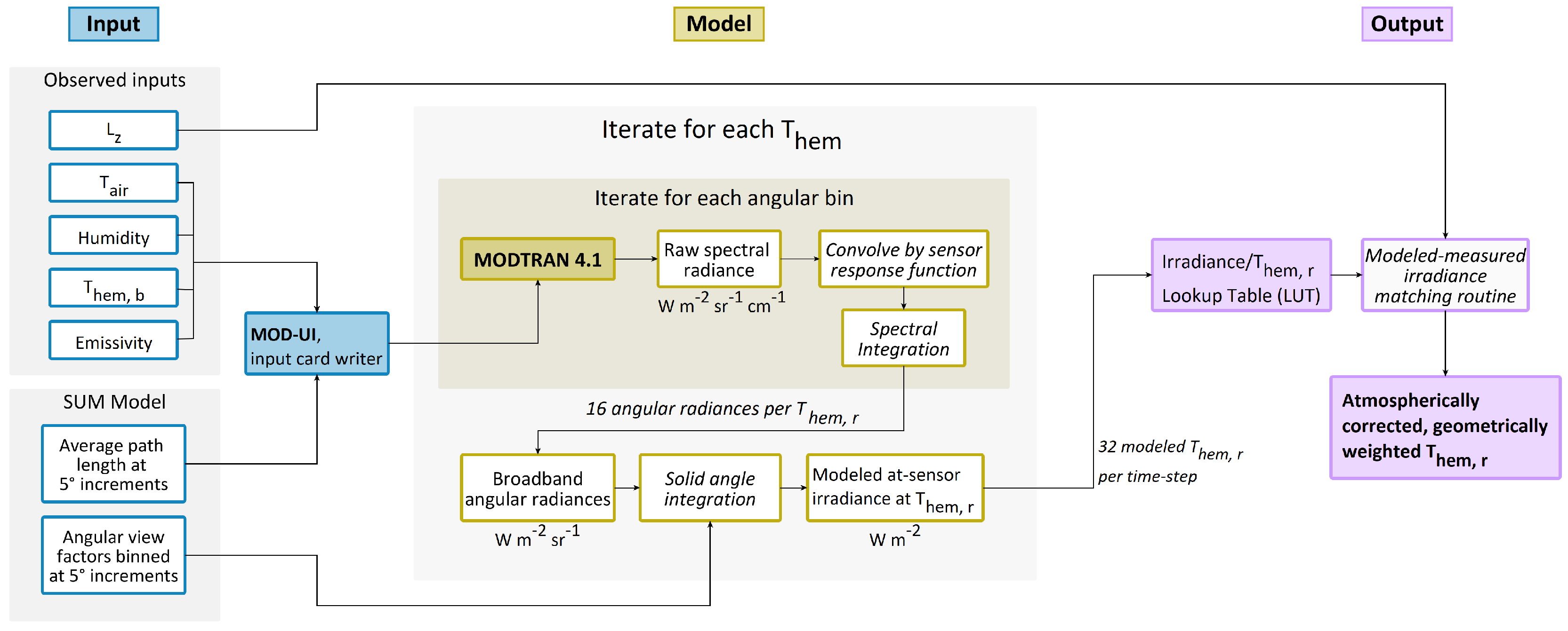
The “rolling lookup-table” method described in this study uses a sensor view model in conjunction with a radiative transfer code to model hemispherical irradiances upwelling from a simplified isothermal three-dimensional representation of the urban surface. In summary, the method (depicted in Figure 3) uses vertical profiles of measured Tair and humidity to model at-sensor spectral radiances at 5 angular increments over the sensor FOV for a predetermined range of possible Them, r at each time-step. Spectral directional radiances are convolved by a pyrgeometer dome transmittance curve, integrated over the sensor waveband, and weighted for their respective angular view factor. Weighted directional radiances are then integrated over the hemisphere and aggregated into a LUT of modeled irradiance—Them, r pairings for each time step, unique to the vertical profile of measured Tair and humidity. Finally, for each time step, measured irradiances are matched with the closest modeled irradiances in the LUT to return an atmospherically corrected radiometric hemispherical surface temperature. This process is repeated at 30 intervals to yield a continuous climatology of urban Them, r. The following sections introduce the study area for which the method was developed and describe the sensor view model, radiative transfer, and post-processing steps of the correction method.
2.1. Study Area
As discussed in Section 1.3, atmospheric correction of longwave irradiances measured from downward-facing, near-ground, wide-FOV sensors must account for complex surface geometry. Thus, routines to retrieve atmospherically corrected urban Them, r from upwelling longwave irradiances are inherently site specific. However, it is important to note that although correction magnitudes described in this paper is not necessarily generalizable, the correction method described in this paper can readily be adapted to different study sites, sensor types, and unique surface geometries.
With methodological generalizability in mind, a “rolling lookup table” atmospheric correction method was developed to retrieve radiometric Them, r for a climatology of upwelling longwave irradiances measured from above the Sperrstrasse street canyon in Basel, Switzerland instrumented as a part of the Basel Urban Boundary Layer Experiment (BUBBLE) [13]. Site location, measured meteorological and radiation variables, and morphological characteristics are included in Table 1. Morphological parameters for the were calculated for a 250 circular area surrounding the study sites using the method described in Grimmond and Oke [20].
For the eight-month period between December 2001 and July 2002 during BUBBLE, a triangular lattice tower was installed within the Sperrstrasse street canyon. Its location was offset towards the southeast facing wall near the along-canyon center of the canyon. Instruments to observe a full suite of meteorological variables and fluxes of heat, mass, and momentum were mounted at various levels on the tower. Profiles of Tair and humidity were measured at seven heights extending from 2.5 to 31.5 above the canyon floor (with the highest observation level at approximately 2.17 times mean roof level). Upwelling and downwelling short/longwave fluxes were obtained from Kipp and Zonen radiometers mounted at the lowest and highest measurement levels, with an additional downward facing pyrgeometer mounted at roof level near the center of the street canyon. In addition, during a summertime intensive observation period (IOP) fron 10th June through 9th July an array of narrow-FOV IRTs was installed to sample representative individual facet surface temperatures (Tfacet). A schematic of the locations of IRTs and pyrgeometers within the Sperrstrasse canyon is included in Figure 4.
The BUBBLE Sperrstrasse site was chosen here for three primary reasons: (1) the site provided a continuous dataset of radiation and meteorological variables over the course of nearly one year for a representative mid-latitude city. This allowed for examination of urban Tsurf the surface urban heat island effect (sUHI), and atmospheric correction magnitudes over a wide range of representative mid-latitude conditions; (2) inclusion of Tfacet over the IOP allows for investigation of the effect of sensor FOV and viewing direction on remote sensed urban Tsurf for common methods of urban Tsurf retrieval; and (3) the site has been used in multiple validation exercises for urban climate models [21,22].
Facet surface temperatures measured during the summertime IOP allow for direct comparison of Them, r to common remote sensed representations of the urban surface calculated from weighted averages of wall (Twall), road (Troad), and roof (Troof) temperatures. Plan and complete aspect ratios are used to derive weightings for nadir remote sensed (Tplan) and complete (Tcomp) representations of urban surface temperature - described in Table 2. Tcomp represents a complete urban Tsurf, where facet temperatures are averaged based on their proportion of the complete urban surface area, while Tplan represents the Sperrstrasse site as viewed by a narrow-FOV remote sensor in the nadir. To facilitate comparison over the IOP, Them, r and Tplan were divided by Tcomp and averaged at each time step over the IOP to yield normalized mean Them, r and Tplan at 30 intervals. Through comparison of Them, r to Tplan and Tcomp we investigate the effect of sensor-surface geometry on remote sensed urban Tsurf and quantify directional biases in common urban Tsurf measurements.
2.2. Modeling Path Lengths of Three-Dimensional Terrain
The sheer number of unique path length geometries inherent with wide-FOV radiometry of urban areas makes full three-dimensional radiative transfer simulation difficult and computationally intensive. In this method, instead of calculating upwelling radiances from each point on the surface to the sensor, radiances are calculated for azimuthally averaged path lengths that represent the average surface-sensor geometry for each solid angle “sector” of the sensor FOV. To visualize this, imagine binning all possible path lengths in three dimensions between two zenith angles (e.g., the solid angle sector bounded by = 90 and = 75) in Figure 2. In a given bin, path lengths running parallel to the canyon axis will be much longer, while those perpendicular to the canyon axis may intersect with walls or rooftops and be much shorter. The mean path length in each bin represents the average distance from the surface to the sensor for the “slice” of the sensor FOV. This simplification reduces the computational time needed to model each irradiance—Them, r pairing, as angular radiances can be computed as a function of zenith angle alone and subsequently weighted and integrated three-dimensionally over the hemisphere.
To calculate surface-sensor geometries, the Surface-Sensor-Sun Urban Model (SUM) [23] is initialized with a simplified, orthogonal three-dimensional DBM that represents surface geometry of the surrounding area. SUM uses a three-dimensional array to represent surface morphology (x, y, and z), with z representing height above the x, y plane. Information describing each cell is included in an additional dimension (in this case, distance from the cell to the sensor). After specifying sensor position and FOV, the model determines which cells have an unobstructed line of sight to the sensor and calculates distance from “seen” patches to the sensor. Path lengths are binned at 5 increments of zenith angle and averaged to return an azimuthally-independent mean path length for each bin. In addition, while retrieving path length geometries, SUM calculates view factors for each solid angle sector, which are later used to weight angular radiances in the hemispherical integration post-processing steps.
In relatively homogeneous urban areas, simplification from three to two dimensions does not reduce accuracy because a pyrgeometer returns a single “bulk” measure of upwelling irradiance—one that is integrated over the sensor FOV. Thus, when atmospheric conditions and surface radiative properties are reasonably constant for a given solid angle sector, there is no functional difference between resolving radiative transfer for every possible path length with its unique Tair and humidity profile and resolving radiative transfer for a single azimuthally averaged atmospheric profile and path length geometry combination. In urban environments that are highly heterogeneous—for instance, in areas with significant heating, ventilation, and air conditioning (HVAC) exhaust or large variations in surface radiative properties—care should be taken when simplifying radiative transfer as emissivity, atmospheric transmittance, and/or Tair may change significantly over the FOV and may not be accurately represented by averaging in each solid angle sector.
2.3. Modeling Hemispherical Irradiances
With path length geometries calculated in SUM, irradiances are modeled for each time step using version 4.1 of the MODerate resolution atmospheric TRANsmission radiative transfer code (MODTRAN) [15]. At each time-step, a range of possible temperatures is specified (Tspec) based on Them, b calculated from the measured irradiance with
defining a minimum Tspec before iterating over
to retrieve a lookup table (LUT) of Tspec.
After the LUT is defined, at-sensor spectral radiances for each path length/zenith angle are modeled at an average urban emissivity of 0.95 [24] over a waveband of 0–2300 for each Tspec. Profiles of Tair and humidity are retrieved from 30 averages of conditions observed at the Sperrstrasse site. Averages of 30 are used over raw 5 values in order to smooth the input Tair and humidities and to cut down on the number of model runs needed to retrieve a long term climatology. The method can be adapted to any time interval. Aerosol, trace gas concentrations, and above-sensor Tair and humidity conditions are defined by the mid-latitude summer standard atmosphere when daytime Tair, max > 10 (the mid-latitude winter profile is substituted on days where Tair, max < 10 ) [25].
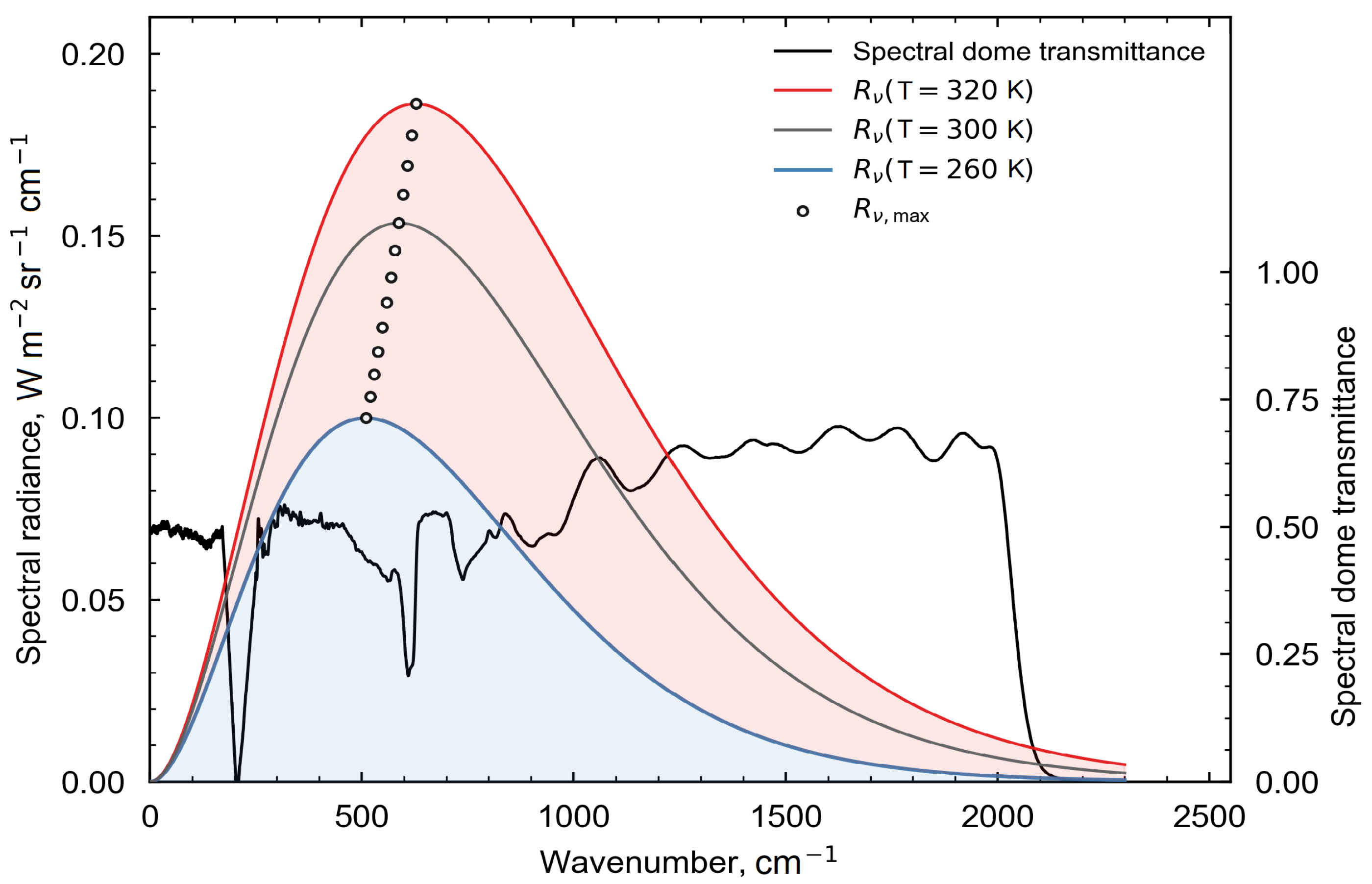
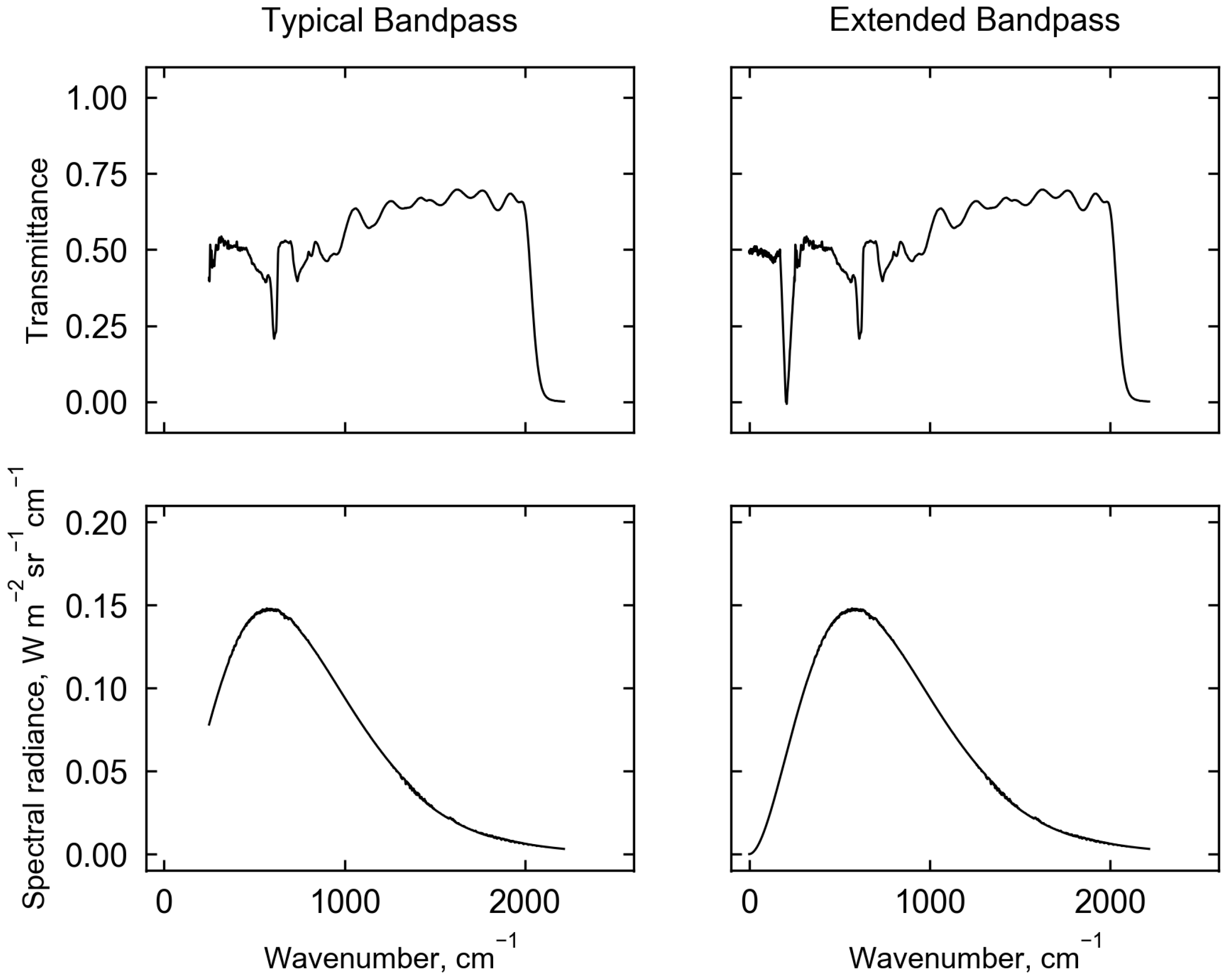
In this method, a “typical” longwave bandpass—approximately 250–2300 (4–42 )—was extended to include much smaller wavenumber (longer wavelengths). This was done for two reasons: (1) to accurately represent broadband spectral longwave emission curves, which show significant emittance in wavenumber smaller than 250 (wavelengths longer than 42 ); and (2) to replicate the spectral signal “seen” by a silicone-domed pyrgeometer, which continues to transmit radiation at wavenumber < 250 (wavelengths > 42 ). A “typical” longwave bandpass underestimates a pyrgeometer signal by approximately 7–10 , depending on emitter temperature. A comparison of ‘typical’ and ‘extended’ longwave bandpasses is shown in Figure 5.
To replicate the signal received by the sensor, at-sensor spectral radiances computed by MODTRAN are convolved by a dome transmittance curve and integrated over the bandpass via
to yield a directional radiance with units for each over a waveband of = 0 to = 2300 . is Planck weighted mean broadband sensor response computed as
where is spectral radiance computed from a Planck function at an approximated emitter temperature and is spectral sensor response.
are then multiplied by their associated angular view factor weighting () and integrated over the hemisphere to yield an irradiance with units with for the target Them, r
is representative of at-sensor irradiance upwelling from the urban surface described in SUM at the target specified temperature Them, r for the measured Tair, humidity, aerosol, and trace gas profile. The process is repeated to retrieve for the range of potential Them, r at the given time-step. Irradiance—Them, r pairings are then aggregated into a LUT. Finally, the measured irradiance is matched with its closest modeled irradiance to yield an atmospherically corrected, radiometric hemispherical surface temperature for the given time step. The workflow is repeated at 30 intervals to yield a time series of Them, r. Atmospheric correction magnitudes can then be calculated as the difference between Them, r and Them, b, with Them, b calculated via Equation (5).
2.4. A Practical Parameterization
To save computational time and facilitate broader use of the method, a parameterization scheme was developed to simplify the correction process. In the parameterization, a suite of radiative transfer simulations is run prior to correction (as opposed to at each time step) to retrieve transmittances () for a range of humidities and path lengths. Tsurf and Tair are held constant in these simulations as they have a relatively small effect on . Simulations for view factor weighted path lengths from 1 m to 48 and water vapor mass densities from 0.1 to 23.5 are included in Appendix A of [26]. Sensor-surface geometry is approximated as a single view factor weighted, azimuthally averaged, surface-to-sensor path length calculated using the SUM [23] and a simplified DBM. This path length represents the average distance from the sensor to the surface as “seen” by the sensor. For each time step, measured humidity is used to infer a hemispherical transmittance () for the approximated surface-sensor geometry. A parameterized Them, r can then be calculated by using measured (in this case, profile averaged) Tair to decompose measured upwelling longwave into irradiance received by the sensor from the surface and from the atmosphere via
where is calculated using a radiative transfer code and is an estimation of the fraction of at sensor measured irradiance emitted by the surface calculated as
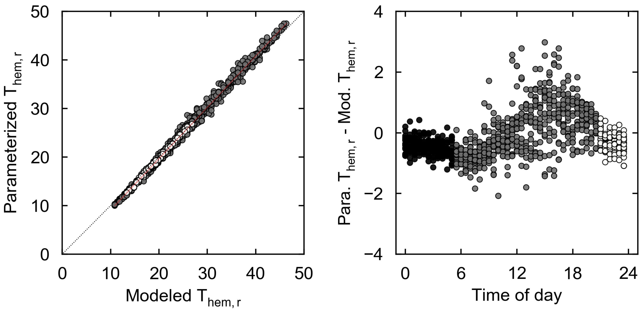
Using this parameterization, a climatology of Them, r for a given surface geometry can be retrieved from approximately 100 simulations as opposed to the many thousands needed for full hemispherical radiative transfer simulation. A variety of online and offline, open and closed source resources are available for radiative transfer simulation [15,27,28], some of which are available for free or at a low cost (e.g., Spectral-Calc, DART). Figure 6 and Table 3 compare Them, r from the “rolling lookup-table” method and the parameterization. Errors are largest during the daytime hours, where the profile averaged Tair overestimates above canyon Tair and underestimates near-surface Tair. Neutral stability in the nighttime and early morning hours reduces these errors significantly as the canyon Tair profile is approximately isothermal.
3. Results
3.1. Method Evaluation
MODTRAN has been shown to effectively model near-ground radiative transfer at urban canyon scale path lengths in two dimensions [31,32]. However, the method described here accounts for complex three-dimensional surface geometry, which can exert strong influence on atmospheric transmittance. In addition, the method includes significant post-processing to weight and integrate point-to-point spectral directional radiances to derive three-dimensional, hemispherical irradiances. Thus, prior to deriving a climatology of urban Them, r, the method was evaluated using profiles of upwelling longwave irradiances measured over a simple flat surface. By testing the method using profiles of upwelling longwave radiation measured over a flat, relatively homogeneous, simple surface, we can assume that, although each sensor has a different set of weightings for each patch on the ground (i.e., the pyrgeometer closest to the ground has a larger view factor for the patch directly below the sensor than the highest pyrgeometer), each sensor should “see” approximately the same surface temperature. Therefore, any differences in the signal between sensor heights is solely a product of atmospheric influence—which should be represented by MODTRAN given concurrent profiles of Tair and humidity. Thus, it follows that, provided urban geometry and path lengths are accurately represented, the method should have similar accuracy over rough urban terrain.
For a continuous 14-day period, profiles of up/downwelling short/longwave radiation, Tair, and humidity measured from 2 , 10 , and 30 were obtained at 30 averages from an instrumented tower in Payerne, Switzerland. The tower, installed over a cultivated field as a part of the Baseline Surface Radiation Network (BSRN), is located approximately 100 southwest of the BUBBLE Sperrstrasse tower and is subject to similar summertime conditions as the study site. The study period was chosen to include a comprehensive range of Tsurf, Tair, humidities, and cloud coverages to represent typical summertime conditions over which atmospheric effects on TIR radiation can vary significantly. To evaluate the method, we used a modified version of the workflow described in Figure 3. First, azimuthally averaged path lengths over a flat surface were calculated in SUM at 5 increments of zenith angle over the sensor FOV for the 10 and 30 sensors. For each time step, Them, b calculated from upwelling longwave measured at 2 was used to model irradiances at 10 and 30 at 30 intervals using concurrent profiles of Tair and humidity. A daytime warm bias of approximately 2 was observed in the 30 Tair measurement, even under high wind velocities when one would expect little vertical difference in temperature and certainly not a strong temperature inversion. The fact that the observed warming bias remains relatively constant in the daytime hours over the 14-day study period prompted a slight modification of the Tair profile to avoid linear interpolation between the 10 Tair and the anomalously warm 30 Tair. Additional Tair measurements were interpolated at 5 increments starting from the 10 measurement, using a lapse rate informed by the difference between Tair at 2 and 10 to replicate typical summertime lapse rates above flat vegetated terrain [24]. When a large warming bias was observed at 30 in the hours after midmorning (when any inversion is likely to have dissipated), the 30 measurement was modified to replicate neutral conditions in the hours around noon, and weakly unstable conditions in the afternoon and evening hours. These modifications provide a smooth Tair profile as one would expect over flat terrain with mild to moderate wind velocities. The nighttime profile was not altered. These modifications are expected to better represent the actual Tair profile in the layer between 10 and 30 than a simple linear interpolation over the layer.
Contrary to the findings in Kotani and Sugita [18], an isothermal atmospheric profile was not sufficient to accurately model upwelling fluxes over flat terrain. Although thermal stratification is relatively small by day in an urban canyon [33]—where strong microscale contrasts in Tsurf foster strong canyon mixing and neutral stability—the large daytime Tsurf − Tair differential and the path length/transmittance gradient can create large differences in upwelling longwave forced by inter-canyon thermal contrasts—a phenomenon termed radiative divergence. By underestimating near-surface Tair and overestimating canopy layer Tair, daytime divergences are underestimated by an isothermal profile. As such, a full canyon Tair and humidity profile is preferred to most accurately model near ground fluxes.
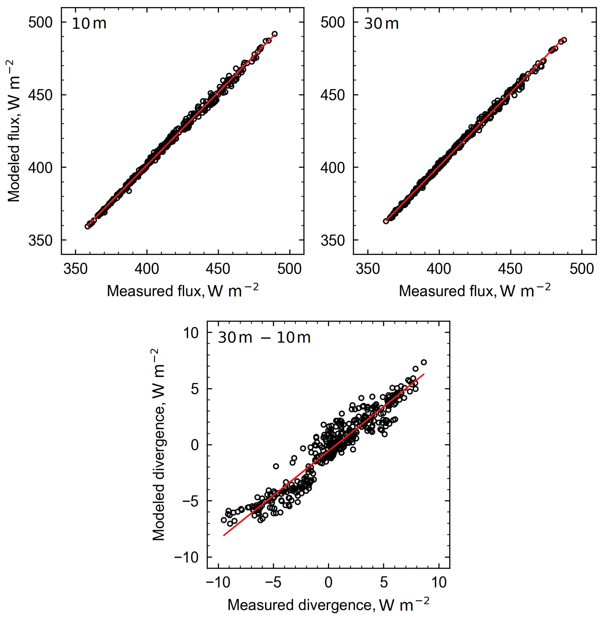
Modeled and measured upwelling longwave at 10 and 30 fluxes and divergences—calculated as the difference between 30 and 10 fluxes—are compared in Figure 7 and Table 4. Both fluxes and divergences show strong correlation. Therefore, we conclude: first, irradiances measured near screen level (approximately 2 above ground level) are not subject to significant atmospheric influence—as Them, b inferred from was sufficient for modeling irradiances at 10 and 30 . As such, Them, b and Them, r are reasonably equal when z = 2 . However, it should be noted that, in urban areas, a 2 sensor is not sufficiently representative of canyon geometry and should not be used to derive urban Them, r. Second, MODTRAN can accurately model longwave fluxes and divergences above a flat, homogeneous surface over a wide range of temperatures, humidities, and cloud coverages and large contrasts in near-ground stability. At 30 under typical summertime profiles of humidity, CO2, and O3, view factor weighted hemispherical transmittance over a flat surface is approximately 55%—meaning 45% of a broadband hemispherical TIR signal at 30 is emitted by the atmosphere, rather than the target surface. As such, it is imperative that Tair profiles are well represented in MODTRAN to accurately model the atmospheric component of remote sensed TIR signal. As profiles of Tair in the layer between the surface and the sensor at the Sperrstrasse site are generally subject to neutral or weakly unstable conditions, with only rare stable stratifications, urban longwave divergences are likely to be smaller than those observed in this evaluation—and well approximated by MODTRAN. Thus, provided path length geometries are accurately replicated by the sensor view model, we can reasonably assume that the method will have similar effectiveness at the urban site. Direct validation of the method in urban environments is difficult as the geometry and heterogeneous surface types of cities (and their associated micro-scale contrasts in Tsurf) are difficult to accurately replicate in radiative transfer models.
3.2. Atmospheric Correction Magnitudes
Atmospheric correction magnitudes binned for season and time of day for the eight-month study period are shown in Figure 8. Summertime correction magnitudes show large day-to-day and diurnal variations. Variation is largest in summer near solar noon, where different synoptic conditions can force correction magnitudes of up to 8 in clear-sky hot conditions and below 0 under cooler overcast conditions. In winter, correction magnitudes display less variance and are smaller—approximately 2 over a range of representative wintertime synoptic conditions.
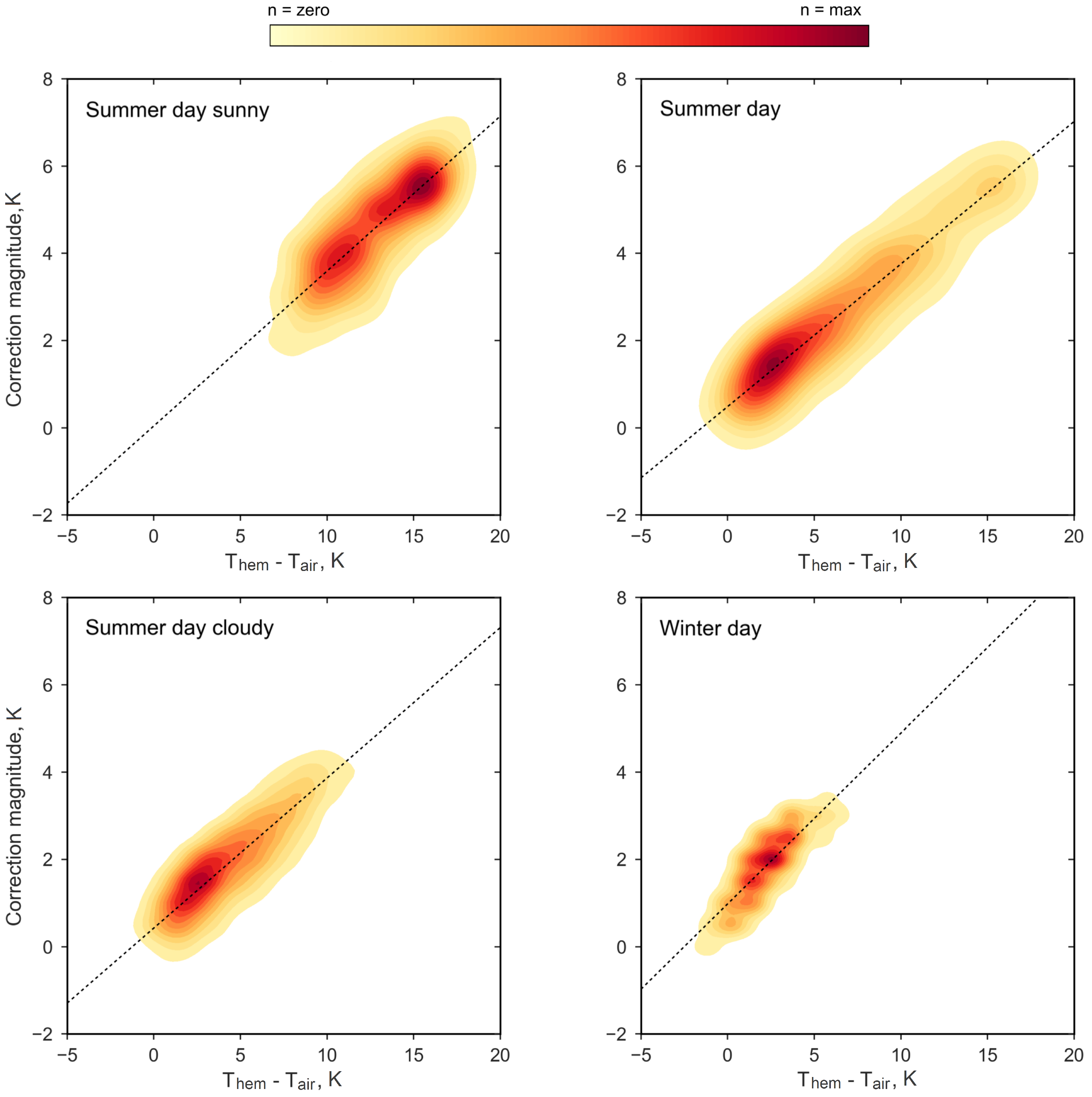
Over both summer and winter seasons, correction magnitudes are strongly correlated with Them, r−air. Figure 9 shows the effect of seasonality and cloud cover on the relationship between correction magnitudes and Them, r−air. The relationship is strongest and most evident in summer when variations in cloud cover can lead to large day-to-day contrasts in solar input and Tsurf−air, which translates into a wide range of correction magnitudes.
Figure 10 illustrates the relationship between correction magnitude and meteorological variables commonly measured as a part of climatological assessments of urban environments. A strong positive relationship is observed between correction magnitudes and incoming solar radiation. Them, r and Tair display more complex relationships with correction magnitude, with a large cluster of observed correction magnitudes situated at a local minimum between 10 and 20 , weakly negative correlation at temperatures lower than 10 , and weakly positive correlation at temperatures greater than 20 . Atmospheric water vapor content did not appear to exert significant control over correction magnitudes.
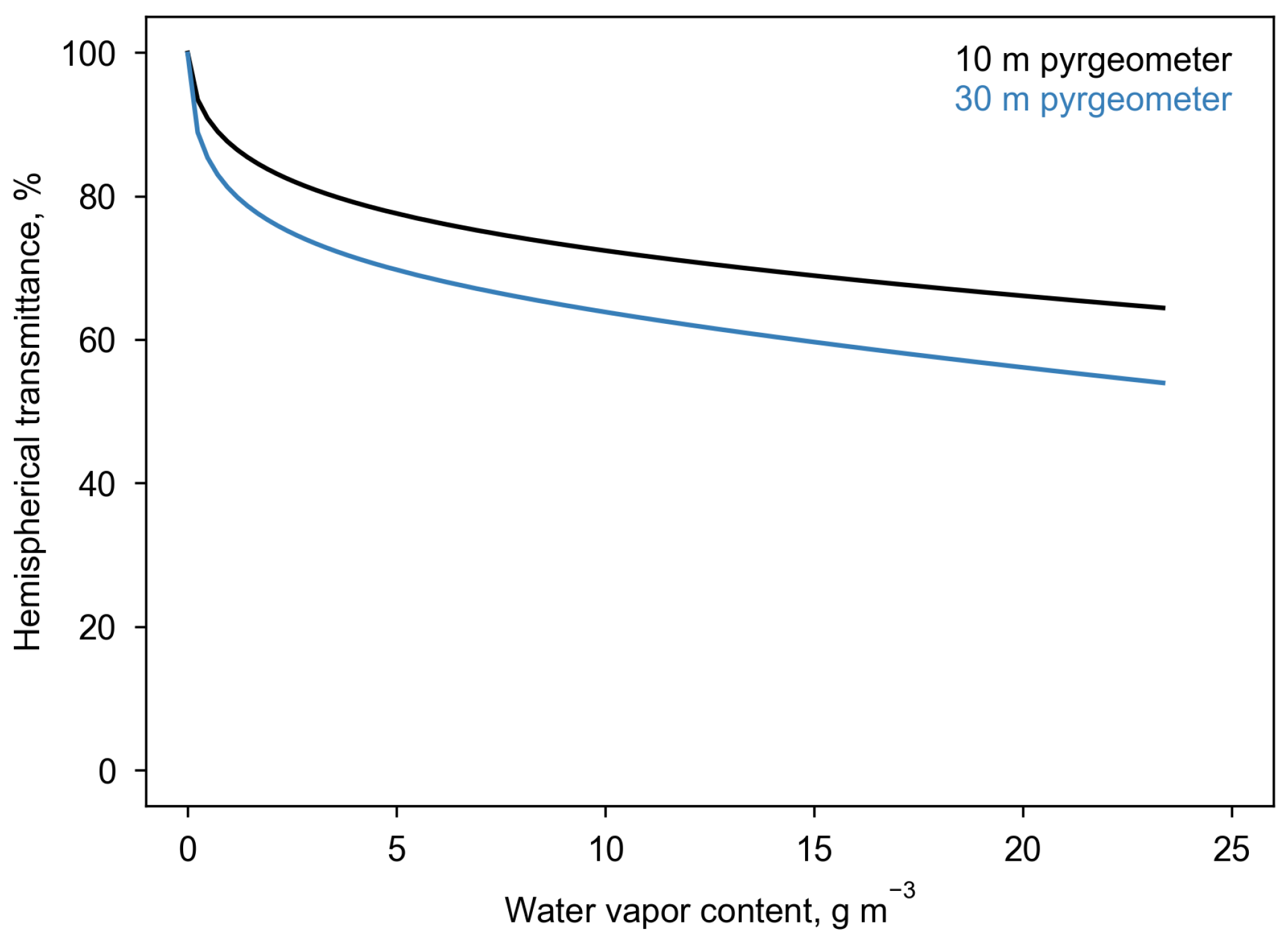
Figure 11 shows hemispherical atmospheric transmittance as a function of vapor pressure for pyrgeometers at 10 and 30 above a hypothetical flat homogeneous surface. Transmittances are modeled in MODTRAN 4.1 as fraction of surface emission reaching the sensor. Hemispherical transmittance falls sharply with increasing vapor pressure between 0 and 5 , but is relatively constant with vapor pressure >5 . This results in the weak correlation observed in Figure 10 between humidity and correction magnitude.
3.3. Comparing Tsurf from Different Sensor Geometries
To illustrate the effect of sensor-surface geometry on remote sensed Tsurf, Figure 12 shows a comparison of mean normalized Them, r and Tplan calculated by dividing Them, r or Tplan by Tcomp at each timestep and averaging over a 14-day subset of the IOP from 26 June 2002 through 9 July 2002 during which all IRTs were operational. In the figure, overestimation of Tcomp is observed at values above one and underestimation by values below one. Both Them, r and Tplan overestimate Tcomp by day and underestimate Tcomp by night. Mean daytime overestimation of Tcomp by Them, r is smaller and less variable than that by Tplan.
Mean normalized Them, r, Tplan, and Tplan−hem, r are shown in Figure 13 along with clear sky and overcast sky case days. While mean Them, r and Tplan display similar overestimations of Tcomp, under clear sky conditions, overestimation by Tplan is much larger than that by Them, r.
4. Discussion
4.1. Controls on Atmospheric Correction Magnitude
Atmospheric correction magnitudes of downward facing pyrgeometers are highly dependent on factors that control Tsurf−air. With a non-zero Tsurf−air, TIR radiation emitted from the surface and absorbed by the atmosphere is re-emitted at a different temperature, modifying the at-sensor TIR signal. Thus, the strength of the Tsurf to Tair differential is directly related to the magnitude of atmospheric effects on a remote sensed TIR signal. This results in a strong positive relationship between atmospheric correction magnitude and Them, r−air. With a non-zero Tsurf−air, TIR radiation emitted from the surface and absorbed by the atmosphere is re-emitted at a different temperature, modifyingair. Results in Figure 9 and Figure 10 show that conditions that maximize microscale surface to atmosphere thermal contrasts result in large correction magnitudes and conditions that suppress differences between Tsurf and Tair show much smaller or negative correction magnitudes.
Of the meteorological variables tested, correction magnitudes are most strongly dependent on solar input. Solar radiation incident on the surface forces microscale thermal contrasts between the surface and the air, directly controlling the Tsurf − Tair difference. The relationships between correction magnitude and Them, r and Tair individually are weaker and more complex. Correction magnitudes are smallest when Them, r and Tair are between approximately 10 and 20 —largely made up of morning and cloudy observations during the summer months where thermal contrasts between Tsurf and Tair are small or weakly negative, forcing small correction magnitudes. During the winter months, a negative relationship between Them, r and Tair and correction magnitudes is observed, likely a result of the effect of shifting spectral emittance curves combined with non-uniform sensor response—discussed in Section 4.2. On clear sky summer days, positive relationships between correction magnitudes and Them, r and Tair are observed as an increased solar input foster higher overall temperatures and large contrasts between Tsurf and Tair.
Results in Figure 8 show significant seasonal and diurnal variation in correction magnitudes. The range of observed correction magnitudes is largest in summer, when a wide range of mid latitude synoptic conditions result in significant contrasts in daytime solar input and consequently large variations in the Tsurf − Tair difference. Maximum correction magnitudes over the study period (often approaching 7 to 8 ) occur frequently near solar noon on clear, hot, humid days, during which intense solar heating of the surface produces a large Tsurf − Tair differential. Minimum correction magnitudes near occur consistently on clear, calm nights following hot days, when Tsurf can dip below Tair, even in urban areas where canyon trapping of radiation reduces cooling rates for both Tsurf and Tair. In winter, decreased variability in overall solar input results in less intense solar heating of the surface and smaller Tsurf − Tair contrasts. Thus, winter correction magnitudes are smaller and more consistent with a mean of approximately 2 .
4.2. The Effect of Non-Uniform Pyrgeometer Spectral Dome Transmittance on Correction Magnitudes
A pyrgeometer’s dome transmittance is spectrally non-uniform. Thus, the “dome effect” a pyrgeometer exerts on an incoming TIR signal changes as a function of emission temperature (Temiss) because the shape of a given spectral radiance curve (R) is temperature dependent. This is illustrated in Figure 14 by comparing the relative peaks and shape of a pyrgeometer dome transmittance curve for several R (Temiss) for a range of typical urban Temiss. Each curve interacts with a different portion of the spectral dome transmittance curve (r) resulting in different effects from the pyrgeometer dome for each Temiss.
When modeling a pyrgeometer signal, it is important to account for the influence of a specific pyrgeometer dome’s spectral transmittance to avoid introducing a temperature dependent bias and to ensure the modeled signal is accurate. As such, the method in this study convolves modeled at-sensor spectral radiances by a spectral dome transmittance function obtained from Kipp and Zonen to accurately model upwelling irradiances as “seen” by the pyrgeometer.
To understand the influence of differential pyrgeometer dome transmittance effects at typical urban Temiss, we use Equation (9) to calculate Planck weighted dome transmittances at 5 intervals from Temiss = 260 to Temiss = 320 , shown in Table 5. varies by approximately 2% over typical urban Temiss, with higher at low Temiss and lower at high Temiss. Although this bias appears small, when comparing observations from multiple pyrgeometer types (each with their own spectral dome transmittance function) and when comparing modeled and measured irradiances, these biases may contribute an additional source of error.
4.3. The Effect of Sensor Sampling Geometry on Remote Sensed Tsurf
Results in Figure 12 and Figure 13 show that sensor sampling regimes can have a significant effect on remote sensed Tsurf. Both Them, r and Tplan overestimate Tcomp by day and underestimate Tcomp by night. These results are consistent with findings in [10,34] observed for clear sky days. However, when analyzed over a time series, over/underestimations from geometric effects are highly dependent on synoptic conditions, particularly for a nadir view of the urban surface. Tplan is much greater than Tcomp under clear sky conditions, with Them, r showing a smaller positive bias. Over half of the Tplan signal from the Sperrstrasse canyon is generated by rooftops that have both a large diurnal Tsurf amplitude and the highest daytime facet Tmax. Undersampling of sloped facets and neglect of wall facets by Tplan also has a significant effect on the daytime clear-sky warming bias, as walls show much cooler daytime Tmax than Troof or Troad and have a moderating effect on Tcomp and Them, r by day, particularly on hot clear sky days. Mean daytime overestimations by Tplan just after solar noon are approximately 4 during the IOP, approaching 8 on the clear sky case day. Them, r shows smaller overestimations of approximately 3 over the 14-day subset of the BUBBLE IOP and 5 on the clear sky case day. Urban Tsurf and the sUHI are often measured from satellite remote sensors that retrieve Tplan exclusively under clear-sky conditions and often sample in the nadir [35,36]. Thus, overestimation of daytime urban Tcomp inherent in the satellite Tsurf record is best represented by Tplan on the clear sky case day.
Nighttime underestimations of Tcomp by nadir and hemispherical views are a result of an undersampling of wall and road facets, respectively, as suggested by Roth et al. [1]. Them, r derived from measured at the Sperrstrasse canyon oversamples the nearest roof and underestimates the canyon floor compared to Tcomp as its location along the canyon axis is skewed towards the south facing wall (rather than the center of the canyon) and its height is approximately 2.17 times mean building height. Sub-optimal sensor placement in the Sperrstrasse canyon—discussed in a sensor placement sensitivity test included in Appendix A—results in a large underestimation of nighttime Tcomp by Them, r. However, nighttime underestimation—and to some extent, daytime overestimation—by Them, r is the combined result of a sampling bias inherent in a hemispherical view of the surface and improper sensor placement. Both of these biases can likely be reduced significantly by adjusting sensor placement to best represent surface geometry.
5. Conclusions
Accurate, geometrically representative, spatially extensive, and temporally continuous thermal remote sensing of complex terrain (urban or otherwise) is difficult. It is unlikely that a single sensor will satisfy spatial, geometric, and temporal goals. Thus, a combination of satellite, aerial, and in situ observational methods has been integral in isolating and elucidating the urban effect on surface temperature and its spatial, temporal, and geometric characteristics. However, neither technological advancement nor critical analysis of these methods has provided a satisfactory answer to the questions posed in Roth et al. [1] viz. urban thermal remote sensing. As such, the true spatial, temporal, and geometric nature of the urban effect on surface temperature remains difficult to measure and quantify.
This paper details a method for urban surface temperature (Tsurf) retrieval using atmospherically corrected hemispherical radiometric surface temperatures derived from continuous near-ground measurements of thermal infrared radiation. Atmospherically corrected, hemispherical urban Tsurf is derived using a method that combines a sensor view model (SUM) to represent urban surface geometry and a point-to-point radiative transfer code (MODTRAN 4.1) to model irradiances upwelling from complex surface terrain in three-dimensions. At each time step, irradiances are modeled using profiles of air temperature (Tair) and water vapor content for a range of possible hemispherical radiometric Tsurf (Them, r). Irradiance–Them, r pairings are aggregated into a lookup table and the measured irradiance is matched with the closest modeled irradiance to retrieve Them, r for a given time step. Repeated at 30 intervals, the method is used to derive an eight-month climatology of urban Them, r from urban irradiances measured as a part of the Basel Urban Boundary Layer Experiment (BUBBLE) in Basel, Switzerland.
Atmospheric corrections are large and show large variations based on sensor–surface–sun geometry and synoptic conditions. Thus, Them derived from irradiances measured at different heights or above different surface geometries may have different atmospheric or dome effects that can confound results. This fact makes clear the need for robust atmospheric correction of Them for surface urban heat island (sUHI) analysis or to retrieve radiometric Them. Correction magnitudes are largest (approaching to 8 ) on hot, clear sky summertime days—with large solar input and high Tsurf and Tair—and smallest (1 to −2 ) by night and under overcast conditions, during which solar input is suppressed and Tsurf and Tair are low. Correction magnitudes are most strongly correlated with the Tsurf to Tair differential and incoming solar radiation and weakly correlated with Them, r and Tair. Water vapor content did not appear to exert strong control over correction magnitudes.
Comparison of Tsurf from nadir (Tplan), hemispherical, and complete (Tcomp) representations of the Basel Sperrstrasse street canyon show that a hemispherical view is more geometrically representative of the complete surface temperature than a sensor viewing in the nadir. However, sensor placement sensitivity tests show that Them, r varies based on sensor placement and height. Overestimations of Tcomp by Tplan and Them, r are greatest under clear sky conditions (up to 8 for Tplan and 5 for Them). This is particularly important when one considers that satellite observations of urban Tsurf are only possible under clear sky conditions (when Tplan is least representative of Tcomp). Significant variability in over/underestimation of Tcomp by Them, r and Tplan based on time of day and synoptic conditions make these biases difficult to generalize to other urban study sites with different surface geometries and characteristics, canyon orientations, and macro climates. However, the measures used to derive Them, r are common to most energy balance assessments and constitute an untapped, but promising, resource to quantify the geometric and temporal biases inherent in satellite remote sensing of TIR radiation from complex terrain.
By providing for time-continuous measurement of urban Tsurf, the method proposed here can be used to provide all weather, long-term seasonal and diurnal analysis of the surface urban heat island effect as demonstrated in [26]. However, it is important to note that use of the method for sUHI analysis requires a matched pair of urban and rural instruments, with the urban measurement taken from a tower three to five times mean building height. This limits use of the method to select local climate zones [37] as towers of optimal height are not feasible in areas with very tall buildings. As a result, the method will not necessarily diagnose the spatial maximum or minimum sUHI. Further care should be taken to accurately represent surface-sensor geometries, the spectral dome characteristics of the pyrgeometer, and the near-ground air temperature and humidity profile in radiative transfer simulations to ensure the correction for atmospheric effects is robust.
Acknowledgments
This project is funded by the Natural Sciences and Engineering Research Council of Canada (NSERC) with support from an NSERC Discovery Grant. Radiometer measurements during BUBBLE were funded by the Swiss Ministry of Education and Science (Grant C00.0068) and collected under Principal Investigators Roland Vogt (Univ. Basel) and Matthias Rotach (Univ. Innsbruck). The BUBBLE dataset was supplied courtesy of Roland Vogt. Evaluation data was supplied courtesy of Laurent Vuilleumier via the PANGEA data publishing portal.
Author Contributions
Michael A. Allen developed the method, its parameterization, and evaluations for both, contributed to method theorization, and produced text and figures (unless otherwise referenced). James A. Voogt contributed to project conceptualization and development of the method, and edited text and figure design. Andreas Christen contributed to project conceptualization and provided data.
Conflicts of Interest
The authors declare no conflict of interest.
Appendix A. Sensor Placement Sensitivity Testing
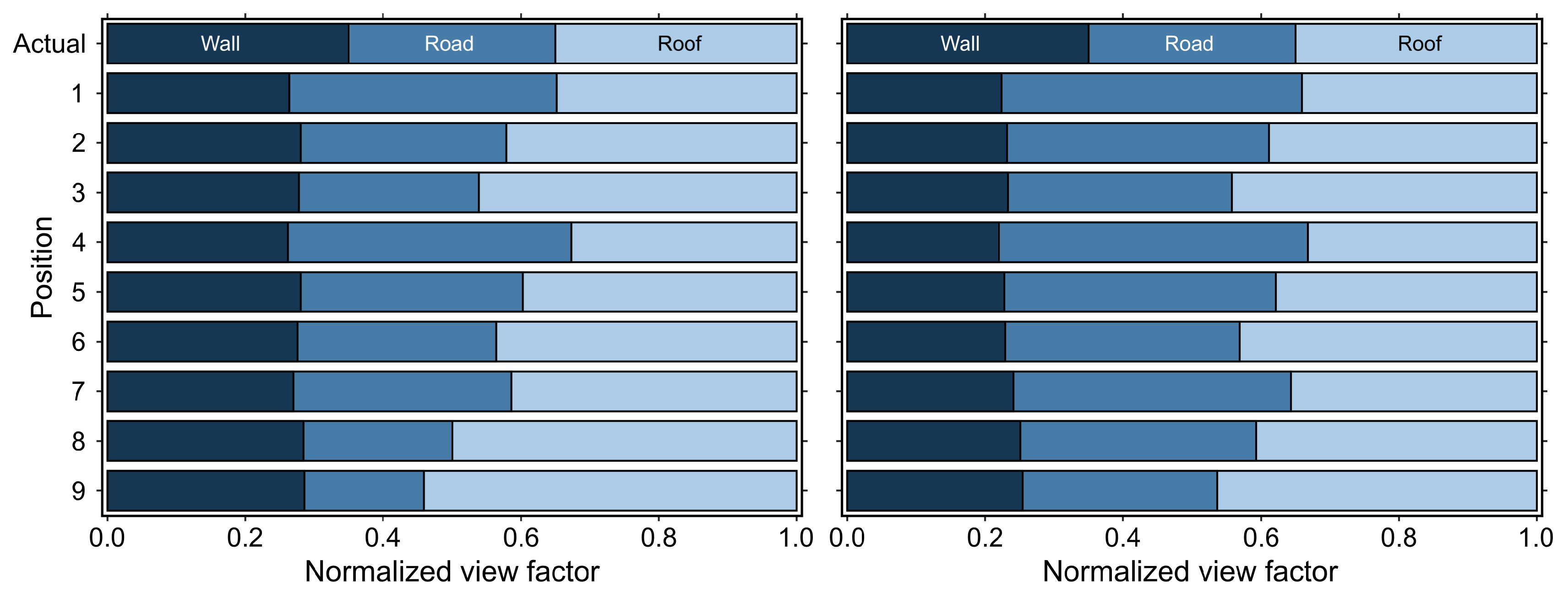
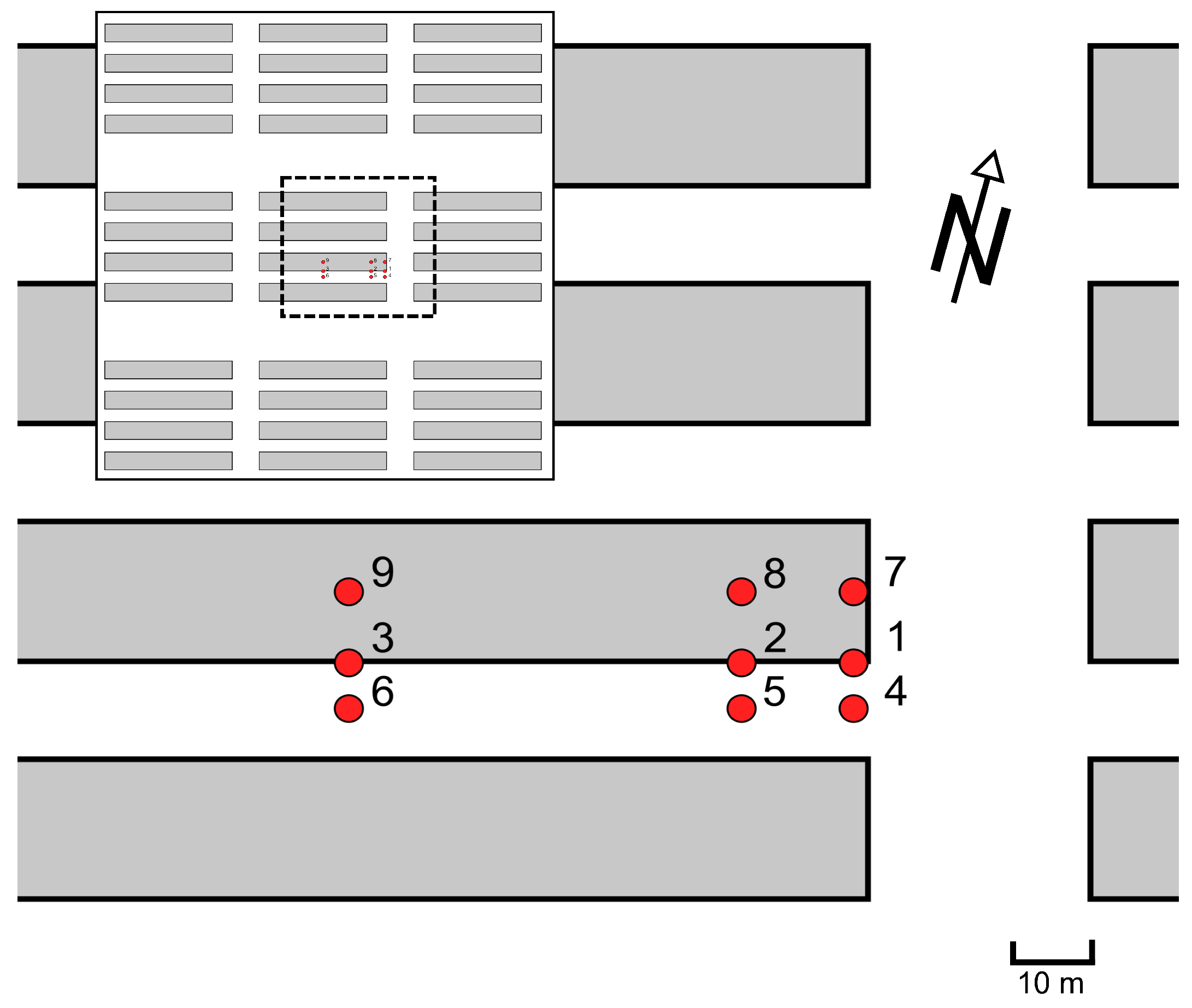
When measured from a near ground downward facing pyrgeometer, upwelling TIR radiation is sensitive to sensor height and position relative to surface geometry [10,38]. Below three times mean roof level, measured TIR radiation varies from a “true”, geometrically representative, TIR signal based on a comparison between facet view factor proportions of the sensor and those of the urban surface. A perfectly geometrically representative remote sensed TIR signal is one measured from a sensor with facet view factor proportions equaling those of the urban surface. For example, for an urban surface made up of 50% wall, 25% road, and 25% roof, a perfectly geometrically representative remote sensed signal would be one “seen” by a sensor with the same fractional facet view factor proportions. For an idealized, orthogonal, block-like urban array, Roberts [38] found that facet view factor proportions—and thus measured TIR radiation—varied significantly with sensor position and height. To investigate the effect of sensor placement on Them, r for a simplified representation of the Sperrstrasse canyon site, we used SUM to vary sensor position over a simplified DBM and calculate normalized view factor proportions for a 160 FOV sensor. For nine sensor positions, shown in Figure A1, facet view factor proportions normalized to unity are shown in Figure A2 for sensor heights of 2.17 and 3 times mean building height. For reference, the location of the pyrgeometer in the Sperrstrasse canyon is best represented by position 3. Approximated actual facet surface area proportions for the Sperrstrasse canyon are included for reference.
Normalized facet view factors in Figure A3 and Figure A4 show large variations based on sensor position at both test heights. At the lower test height, varying sensor position perpendicular to the canyon axis, positions at the canyon center (positions 4, 5, and 6) are most representative of actual facet view factors, with decreasing representivity at the edge of the canyon (positions 1, 2, and 3), and over the rooftops (positions 7, 8, and 9). Moving the sensor parallel to the canyon axis, positions slightly offset from the roof edge (positions 2, 5, and 8) agree most closely with actual canyon surface area proportions, with decreasing representivity in positions further from the roof edge. Roof and road view factor proportions are most strongly affected by sensor placement. Positions directly over buildings show large biases towards roof view factors and positions in the center of the canyon showing slight biases towards road facets. In all positions, roof view factor was overestimated (save position 4), and wall view factor was underestimated.
Figure A1.
A plan view of the simplified digital building model showing the nine test sensor placements. Actual sensor placement at the Sperrstrasse canyon is approximated by number 3.
Figure A1.
A plan view of the simplified digital building model showing the nine test sensor placements. Actual sensor placement at the Sperrstrasse canyon is approximated by number 3.

Figure A2.
Normalized wall, road, and roof view factors for nine sensor positions viewing the simplified street canyon array from 2.17 (left) and 3 (right) times mean building height. The lower sensor height was chosen to represent the height of the pyrgeometer above the Sperrstrasse street canyon. The slightly higher height was chosen to represent view factor proportions one would expect with the same sensor placed at a more ideal height as suggested in Adderley et al. [10] and Roberts [38]. Actual normalized view factors refer to surface area proportions for the three facet types in the Sperrstrasse street canyon.
Results in Adderley et al. [10] and Roberts [38] show that sensitivity to sensor placement decreases as sensor height increases. Depending on surface geometry, sensor view factor proportions and the TIR signal “seen” by a sensor become spatially invariant at heights above approximately 3–5 times mean building height. Results from the higher sensor test height support findings in Adderley et al. [10] and Roberts [38], with decreased spatial variance in facet view factor proportions across the nine sensor positions. However, increased spatial stability in view factor proportions does not necessarily entail increased geometric representivity. For all sensor placements, road view factor proportion is increased and wall view factor is reduced. This results in large overestimations of road view factor for nearly all positions except positions 3 and 9, which include a large overestimation of roof view factor. Thus, although increasing sensor height does reduce spatial variance, it can lead to decreased representivity for some positions—in this case, positions 1 and 4.
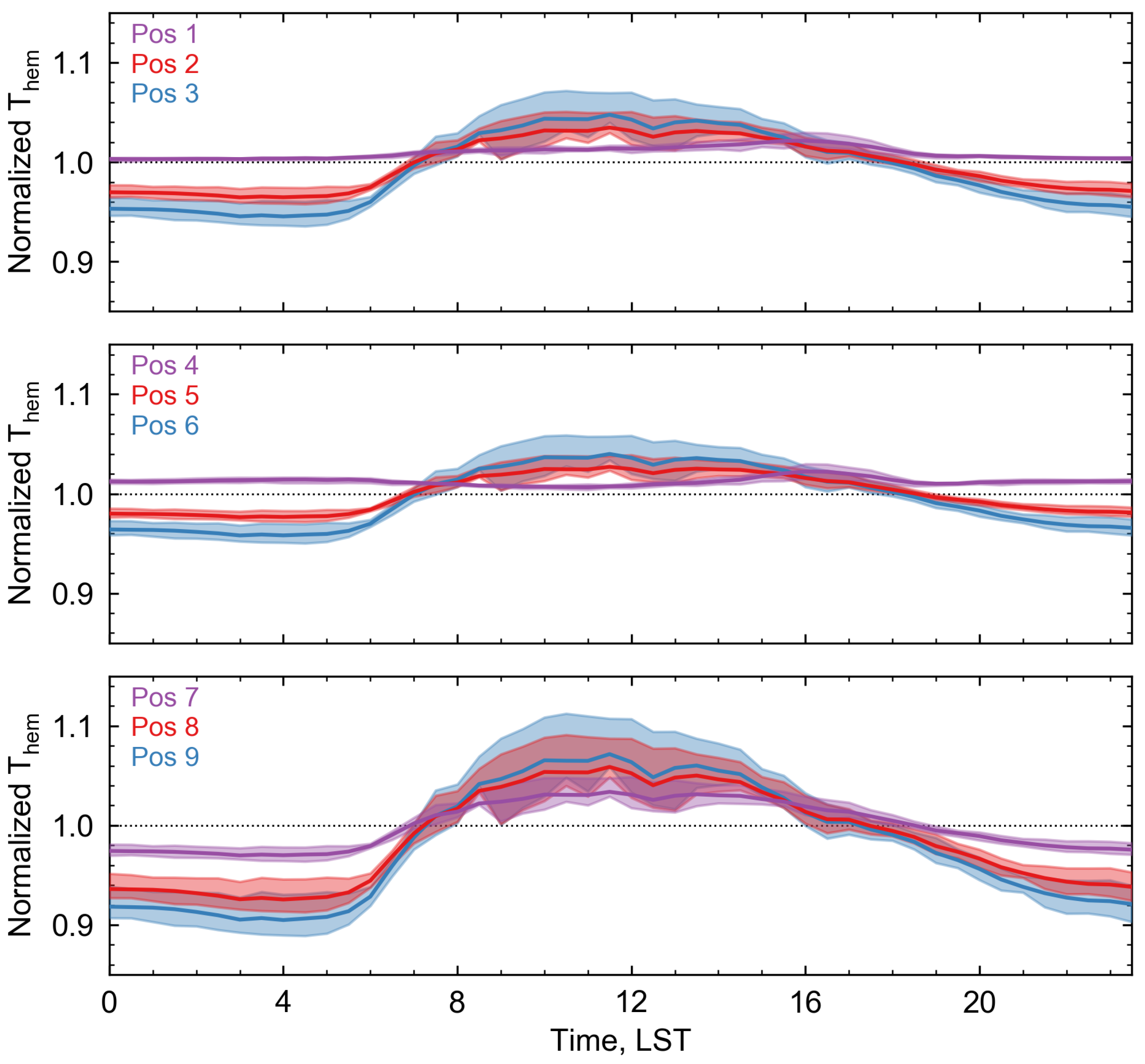
To visualize how sensor placement affects Them, r retrieved via the method detailed in this study, Them, r is inferred using wall, roof, and road view factors calculated in SUM for the two sensor heights to compute a weighted average of Twall, Troad, and Troof for each sensor position at 30 intervals over the IOP. Temperatures are normalized by Tcomp and averaged at each time step over the IOP, the results of which are shown in Figure A3 and Figure A4. As is the case with view factor proportions, Them, r is highly dependent on sensor placement. For the lower sensor height, as predicted by view factor proportions, positions at the center of the canyon (positions 4, 5, and 6) and edge of the building (positions 1, 4, and 7) follow Tcomp most closely. By day, all sensor positions overestimate Tcomp, from a systemic bias towards rooftop facets. The degree of overestimation is largely determined by rooftop view factor, with larger overestimations coming from positions most biased towards hot rooftop surfaces. At night, most sensor positions (save position 4) underestimate Tcomp, again from a bias towards cool rooftop facets. Position 4 weakly overestimates nighttime Tcomp, from a slight view factor bias towards road facets with suppressed nocturnal cooling from canyon radiation trapping.
Figure A3.
Mean Them, r normalized against Tcomp for each sensor position over the 14-day subset of the IOP for a sensor height of 2.17 times mean building height. Shaded area indicates quartiles 1–3.
Figure A3.
Mean Them, r normalized against Tcomp for each sensor position over the 14-day subset of the IOP for a sensor height of 2.17 times mean building height. Shaded area indicates quartiles 1–3.

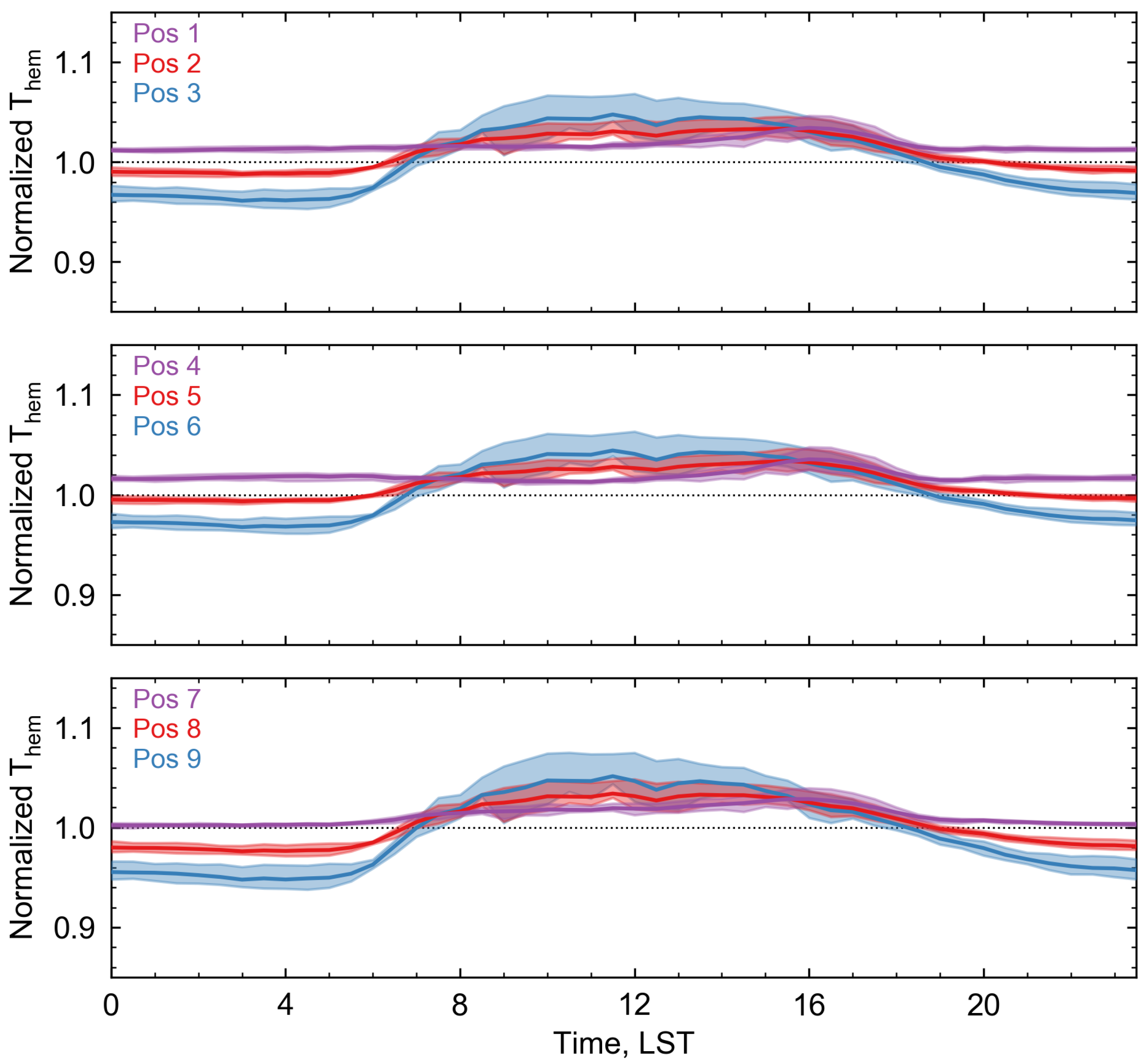
At the higher test height, Them, r is more representative of Tcomp for positions 2, 3, and 5–9. Them, r from positions 1 and 4 display a slight systematic overestimation of Tcomp. For these positions, although roof view factor proportion is well represented, road view factor is significantly overestimated, oversampling warmer nighttime road temperatures. For all other positions, daytime overestimation and nighttime underestimation of Tcomp is reduced. Thus, as is the case with view factor proportions, at the higher test height, Them, r is more spatially stable.
Both Roberts [38] and Adderley et al. [10] did not find a perfectly representative sensor position for typical low- and mid-rise urban street canyons; this is supported by sensitivity testing performed in this study. As such, under conditions with strong microscale spatial contrasts in Tsurf, Them, r is unlikely to be equal to Tcomp regardless of pyrgeometer placement. However, sensor view models, such as SUM, can be used to optimize sensor placement with information about surface geometry to retrieve the best estimation of measured irradiances and derived Them, r for a given surface geometry.
Figure A4.
Mean Them, r normalized against Tcomp for each sensor position over the 14-day subset of the IOP for a sensor height of three times mean building height. Shaded area indicates quartiles 1–3.
Figure A4.
Mean Them, r normalized against Tcomp for each sensor position over the 14-day subset of the IOP for a sensor height of three times mean building height. Shaded area indicates quartiles 1–3.

References
- Roth, M.; Oke, T.R.; Emery, W. Satellite-derived urban heat islands from three coastal cities and the utilization of such data in urban climatology. Int. J. Remote Sens. 1989, 10, 1699–1720. [Google Scholar] [CrossRef]
- Liu, L.; Zhang, Y. Urban heat island analysis using the landsat TM data and ASTER Data: A case study in Hong Kong. Remote Sens. 2011, 3, 1535–1552. [Google Scholar] [CrossRef]
- Peng, S.; Piao, S.; Ciais, P.; Friedlingstein, P.; Ottle, C.; Bréon, F.M.; Nan, H.; Zhou, L.; Myneni, R.B. Surface urban heat island across 419 global big cities. Environ. Sci. Technol. 2012, 46, 696–703. [Google Scholar] [CrossRef] [PubMed]
- Wang, H.; Zhang, Y.; Tsou, J.; Li, Y. Surface Urban Heat Island Analysis of Shanghai (China) Based on the Change of Land Use and Land Cover. Sustainability 2017, 9, 1538. [Google Scholar] [CrossRef]
- Voogt, J.A.; Oke, T.R. Complete urban surface temperatures. J. Appl. Meteorol. 1997, 36, 1117–1132. [Google Scholar] [CrossRef]
- Bastiaanssen, W.G.M.; Meneti, M.; Feddes, R.A.; Holtslag, A.A.M. A remote sensing surface energy balance algorithm for land (SEBAL): Formulation. J. Hydrol. 1998, 212–213, 198–212. [Google Scholar] [CrossRef]
- Yamaguchi, Y.; Kato, S. Analysis of urban heat-island effect using ASTER and ETM+ Data: Separation of anthropogenic heat discharge and natural heat radiation from sensible heat flux. Remote Sens. Environ. 2005, 99, 44–54. [Google Scholar]
- Frey, C.M.; Rigo, G.; Parlow, E. Urban radiation balance of two coastal cities in a hot and dry environment. Int. J. Remote Sens. 2007, 28, 2695–2712. [Google Scholar] [CrossRef]
- Stoll, M.J.; Brazel, A.J. Surface-air temperature relationship in the urban environment of Phoenix, Arizona. Phys. Geogr. 1992, 13, 160–179. [Google Scholar]
- Adderley, C.; Christen, A.; Voogt, J.A. The effect of radiometer placement and view on inferred directional and hemispheric radiometric temperatures of an urban canopy. Atmos. Meas. Tech. 2015, 8, 1891–1933. [Google Scholar] [CrossRef]
- Voogt, J.A.; Oke, T.R. Radiometric temperatures of urban canyon walls obtained from vehicle traverses. Theor. Appl. Climatol. 1998, 60, 199–217. [Google Scholar] [CrossRef]
- Voogt, J.A.; Oke, T.R. Effects of urban surface geometry on remotely-sensed surface temperature. Int. J. Remote Sens. 1998, 19, 895–920. [Google Scholar] [CrossRef]
- Rotach, M.W.; Vogt, R.; Bernhofer, C.; Batchvarova, E.; Christen, A.; Clappier, A.; Feddersen, B.; Gryning, S.E.; Martucci, G.; Mayer, H.; et al. BUBBLE—An Urban Boundary Layer Meteorology Project. Theor. Appl. Climatol. 2005, 81, 231–261. [Google Scholar] [CrossRef]
- Leroyer, S.; Bélair, S.; Mailhot, J.; Strachan, I.B. Microscale numerical prediction over Montreal with the Canadian external urban modeling system. J. Appl. Meteorol. Climatol. 2011, 50, 2410–2428. [Google Scholar] [CrossRef]
- Berk, A.; Bernstein, L.S.; Robertson, D.C. MODTRAN: A Moderate Resolution Model for LOWTRAN7; Technical Report GL-TR-89-0122; United States Air Force: Hanscom Air Force Base, Middlesex County, MA, USA, 1987. [Google Scholar]
- Norman, J.M.; Becker, F. Terminology in thermal infrared remote sensing of natural surfaces. Agric. For. Meteorol. 1995, 77, 153–166. [Google Scholar] [CrossRef]
- Meier, F.; Scherer, D.; Richters, J.; Christen, A. Atmospheric correction of thermal-infrared imagery of the 3-D urban environment acquired in oblique viewing geometry. Atmos. Meas. Tech. 2011, 4, 909–922. [Google Scholar] [CrossRef]
- Kotani, A.; Sugita, M. Concise formulae for the atmospheric correction of hemispherical thermal radiation measured near the ground surface. Water Resour. Res. 2009, 45, 1–7. [Google Scholar] [CrossRef]
- Kneizys, F.X.; Anderson, G.P.; Shettle, E.P.; Gallery, W.O.; Abreu, L.W.; Selby, J.E.A.; Chetwynd, J.H.; Clough, S.A. Users Guide to LOWTRAN 7; Technical Report AFGL-TR-88-0177; Air Force Geophysics Laboratory: Bedford, MA, USA, 1988. [Google Scholar]
- Grimmond, S.; Oke, T.R. Aerodynamic Properties of Urban Areas Derived from Analysis of Surface Form. J. Appl. Meteorol. 1999, 38, 1262–1292. [Google Scholar] [CrossRef]
- Hamdi, R.; Schayes, G. Validation of the Martilli’s Urban Boundary Layer Scheme with measurements from two mid-latitude European cities. Atmos. Chem. Phys. Discuss. 2005, 5, 4257–4289. [Google Scholar] [CrossRef]
- Mauree, D.; Blond, N.; Kohler, M.; Clappier, A. On the Coherence in the Boundary Layer: Development of a Canopy Interface Model. Front. Earth Sci. 2017, 4, 1–12. [Google Scholar] [CrossRef]
- Soux, A.; Voogt, J.A.; Oke, T.R. A model to calculate what a remote sensor ‘sees’ of an urban surface. Bound.-Layer Meteorol. 2004, 111, 109–132. [Google Scholar] [CrossRef]
- Oke, T.R. Boundary Layer Climates; Routledge Books: Abingdon, UK, 1987; pp. 1–435. [Google Scholar]
- Kantor, A.J.; Cole, A.E. Mid-latitude atmospheres, winter and summer. Geofis. Pura Appl. 1962, 53, 171–188. [Google Scholar] [CrossRef]
- Allen, M.A. A Method for Hemispherical Ground Based Remote Sensing of Urban Surface Temperatures. Master’s Thesis, University of Western Ontario, London, ON, Canada, 2017. [Google Scholar]
- Gastellu-Etchegorry, J.P.; Demarez, V.; Pinel, V.; Zagolski, F. Modeling radiative transfer in heterogeneous 3-D vegetation canopies. Remote Sens. Environ. 1996, 58, 131–156. [Google Scholar] [CrossRef]
- Buehler, S.A.; Eriksson, P.; Kuhn, T.; von Engeln, A.; Verdes, C. ARTS, the atmospheric radiative transfer simulator. J. Quant. Spectrosc. Radiat. Transf. 2005, 91, 65–93. [Google Scholar] [CrossRef]
- Willmott, C.J.; Ackleson, S.G.; Davis, R.E.; Feddema, J.J.; Klink, K.M.; Legates, D.R.; O’Donnell, J.; Rowe, C.M. Statistics for the evaluation and comparison of models. J. Geophys. Res. 1985, 90, 8995. [Google Scholar] [CrossRef]
- Willmott, C.J.; Robeson, S.M.; Matsuura, K. A refined index of model performance. Int. J. Climatol. 2012, 32, 2088–2094. [Google Scholar] [CrossRef]
- Hoch, S. Radiative Flux Divergence in the Surface Boundary Layer from Observational and Model Perspectives. Ph.D. Thesis, ETH Zurich, Zurich, Switzerland, 2005. [Google Scholar]
- Hoch, S.; Calanca, P.; Philipona, R.; Ohmura, A. Year-round observation of longwave radiative flux divergence in Greenland. J. Appl. Meteorol. Climatol. 2007, 46, 1469–1479. [Google Scholar] [CrossRef]
- Nakamura, Y.; Oke, T.R. Wind, temperature and stability conditions in an east-west oriented urban canyon. Atmos. Environ. 1988, 22, 2691–2700. [Google Scholar] [CrossRef]
- Voogt, J.A.; Oke, T.R. Thermal remote sensing of urban climates. Remote Sens. Environ. 2003, 86, 370–384. [Google Scholar] [CrossRef]
- Imhoff, M.L.; Zhang, P.; Wolfe, R.E.; Bounoua, L. Remote sensing of the urban heat island effect across biomes in the continental USA. Remote Sens. Environ. 2010, 114, 504–513. [Google Scholar] [CrossRef]
- Streutker, D. Satellite-measured growth of the urban heat island of Houston, Texas. Remote Sens. Environ. 2003, 85, 282–289. [Google Scholar] [CrossRef]
- Stewart, I.D.; Oke, T.R. Local climate zones for urban temperature studies. Bull. Am. Meteorol. Soc. 2012, 93, 1879–1900. [Google Scholar] [CrossRef]
- Roberts, S. Three-Dimensional Radiation Flux Source Areas in Urban Areas. Ph.D. Thesis, University of British Columbia, Vancouver, BC, Canada, 2010. [Google Scholar]
Figure 1.
Spectral transmission of longwave radiation as a function of path length. Model results from MODTRAN 4.1 [15] for radiance emitted from a planar surface at 300 through a standard atmosphere with absolute humidity of 8 . Sampled at heights of 1, 5, 10, 15, 20, 25, and 30 .
Figure 1.
Spectral transmission of longwave radiation as a function of path length. Model results from MODTRAN 4.1 [15] for radiance emitted from a planar surface at 300 through a standard atmosphere with absolute humidity of 8 . Sampled at heights of 1, 5, 10, 15, 20, 25, and 30 .
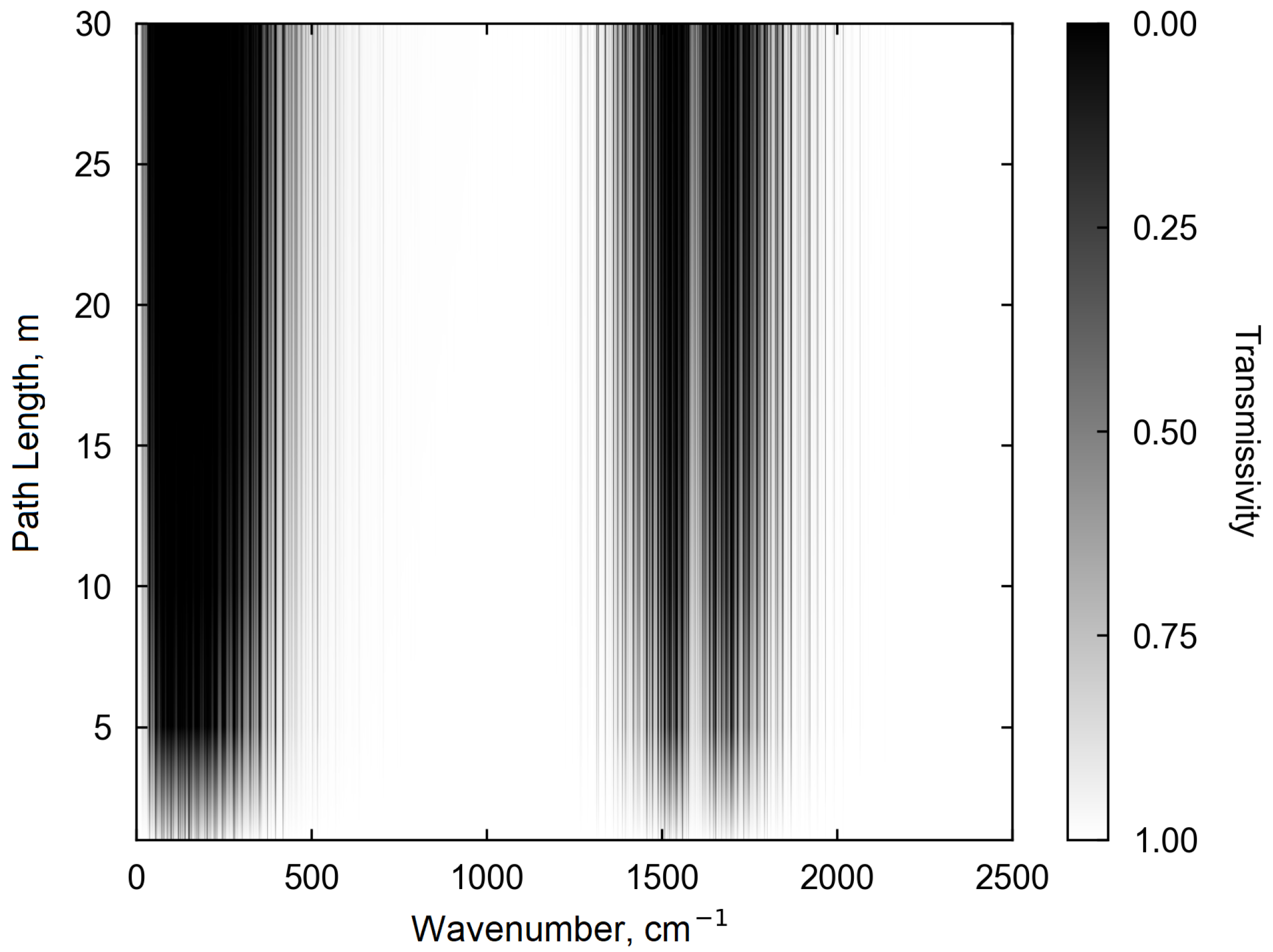
Figure 2.
Variable path geometry inherent with wide field-of-view near-ground sensor visualized over an idealized two-dimensional urban area.
Figure 2.
Variable path geometry inherent with wide field-of-view near-ground sensor visualized over an idealized two-dimensional urban area.
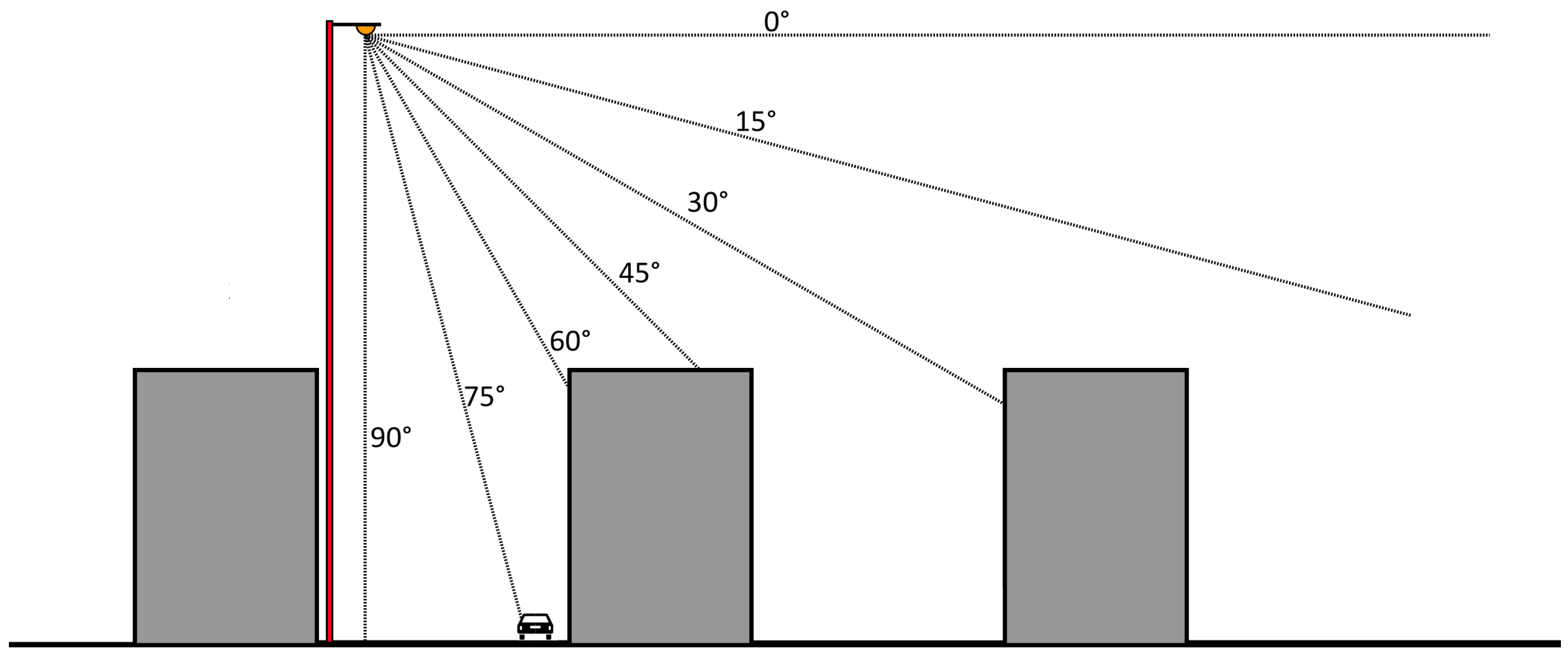
Figure 3.
A workflow schematic depicting the input, model, and output-processing steps of a “rolling lookup table method” for hemispherical radiometric surface temperature retrieval. Italicized text indicates action.
Figure 3.
A workflow schematic depicting the input, model, and output-processing steps of a “rolling lookup table method” for hemispherical radiometric surface temperature retrieval. Italicized text indicates action.

Figure 4.
A schematic showing the thermal infrared radiation instrument setup at the Sperrstrasse urban canyon. Pyrgeometer locations and infrared thermometer FOVs for roof, wall, and road facets are indicated. Only instruments relevant to this work are included in the schematic. The canyon photo is taken viewing from the same direction as the schematic.
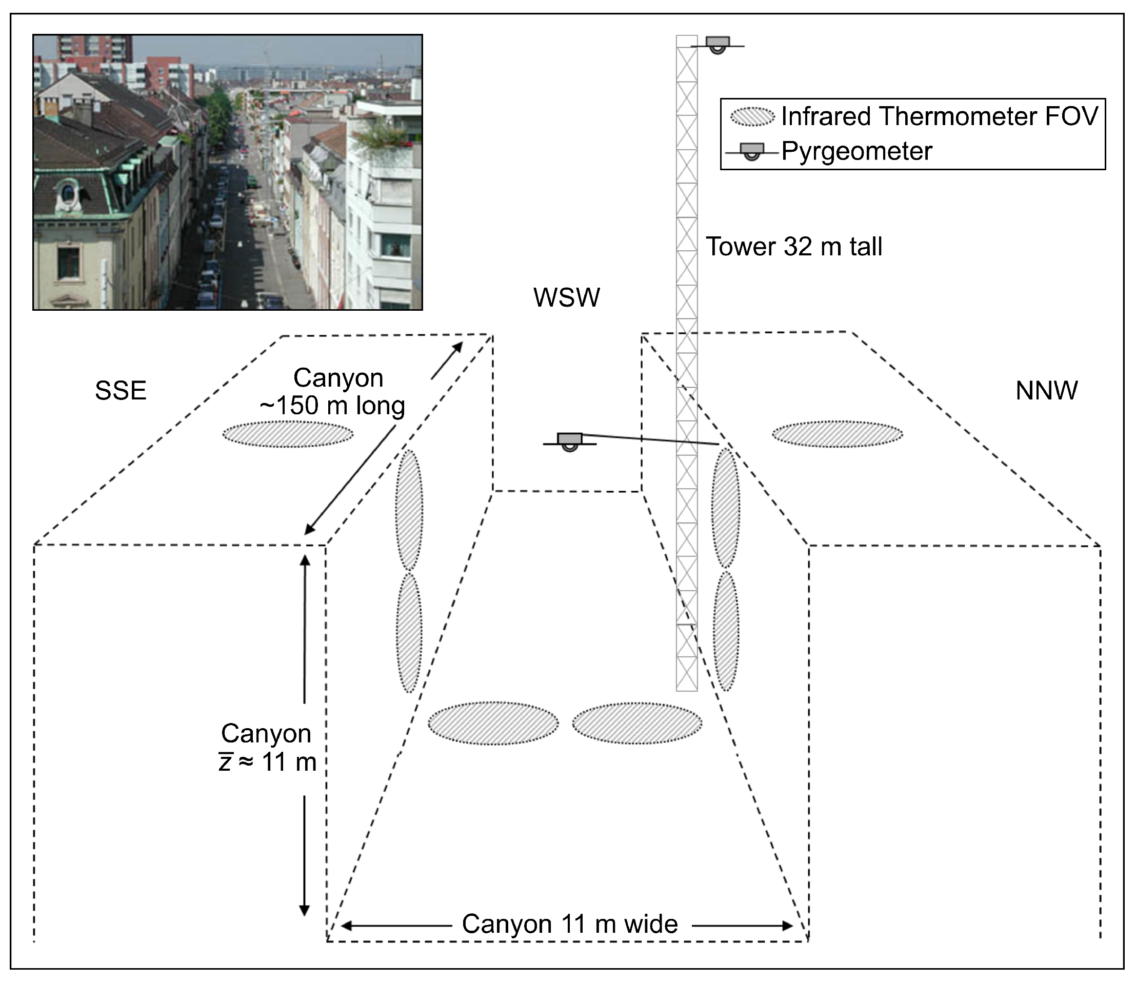
Figure 5.
A comparison of dome transmittance for the model CG3 Kipp and Zonen silicone domed pyrgeometer on the CNR01 4-component system used during BUBBLE (data supplied by Kipp and Zonen, pers. comm.) and at-sensor radiance (Tsurf = 300 , Tair = 300 , z = 30 ) for “typical” and extended bandpasses.

Figure 6.
Modeled Them, r versus Them, r derived via the parameterization scheme. Shading indicates time of day (black is midnight through 5:00 a.m. local standard time, grey is 5:30 a.m. through 8:00 p.m. LST, white is 8:30 p.m. through 11:30 p.m. LST).
Figure 6.
Modeled Them, r versus Them, r derived via the parameterization scheme. Shading indicates time of day (black is midnight through 5:00 a.m. local standard time, grey is 5:30 a.m. through 8:00 p.m. LST, white is 8:30 p.m. through 11:30 p.m. LST).

Figure 7.
A comparison of 10 and 30 measured and modeled longwave fluxes and divergences—calculated as the difference between 30 and 10 fluxes—over the 14-day evaluation period at Payerne, Switzerland.
Figure 7.
A comparison of 10 and 30 measured and modeled longwave fluxes and divergences—calculated as the difference between 30 and 10 fluxes—over the 14-day evaluation period at Payerne, Switzerland.

Figure 8.
Atmospheric correction magnitudes calculated as the difference between Them, r and Them, b calculated from irradiances measured at 31.5 for the duration of the study period at Sperrstrasse canyon. Grey shading indicates average nighttime for the interval. The red line indicates mean correction magnitude at each time step. Box edges represent the 25th and 75th percentiles with whiskers representing one standard deviation from the mean.
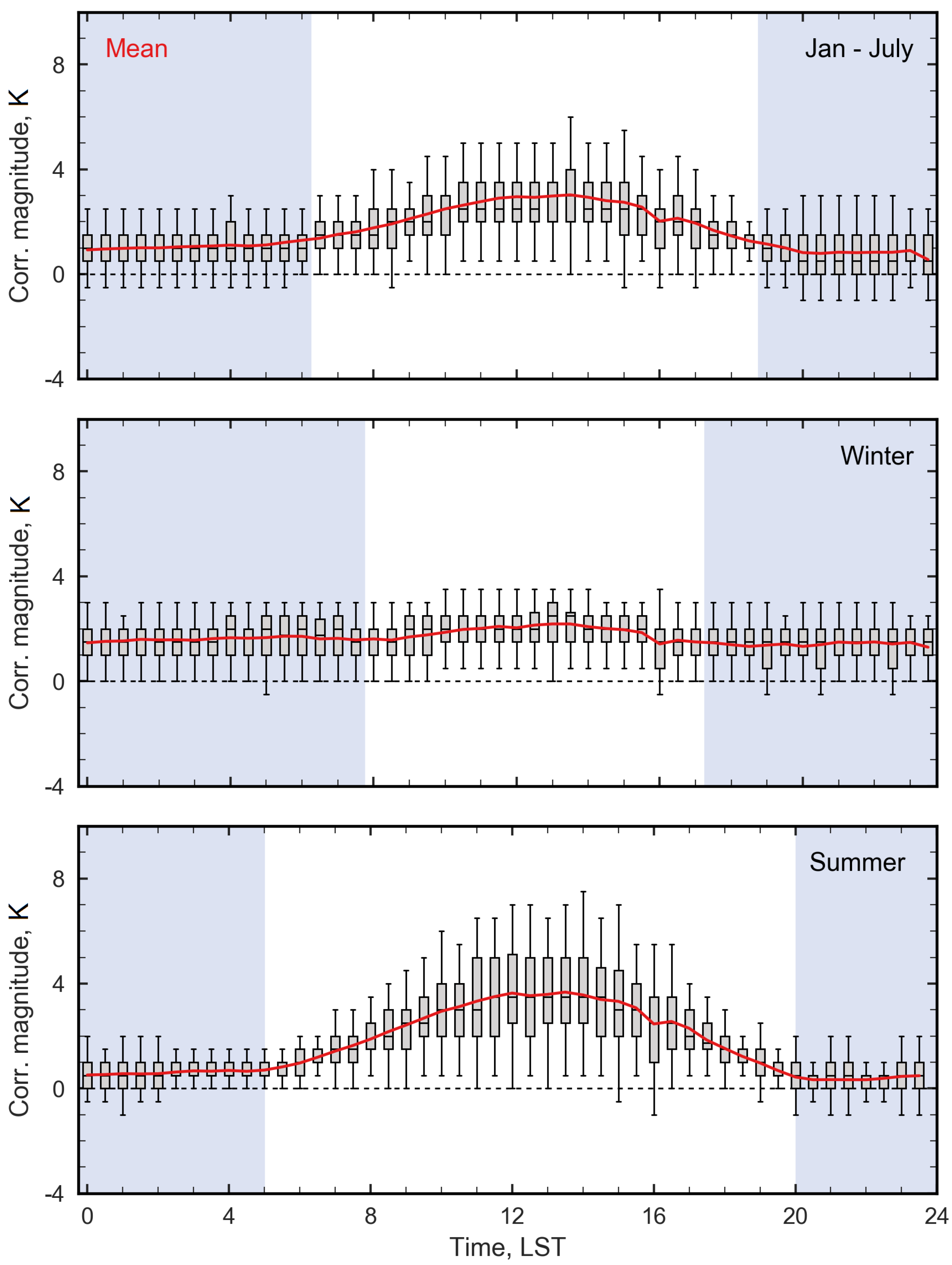
Figure 9.
Correction magnitude versus Them, r−air binned for cloudy and sunny conditions during the daytime hours of the summer months (May 2002–July 2002), and for winter (December 2001–March 2002) and summer seasons.
Figure 9.
Correction magnitude versus Them, r−air binned for cloudy and sunny conditions during the daytime hours of the summer months (May 2002–July 2002), and for winter (December 2001–March 2002) and summer seasons.

Figure 10.
Correction magnitude versus incoming shortwave, Them, r, Tair, and water vapor content for the daytime hours of the study period.
Figure 10.
Correction magnitude versus incoming shortwave, Them, r, Tair, and water vapor content for the daytime hours of the study period.
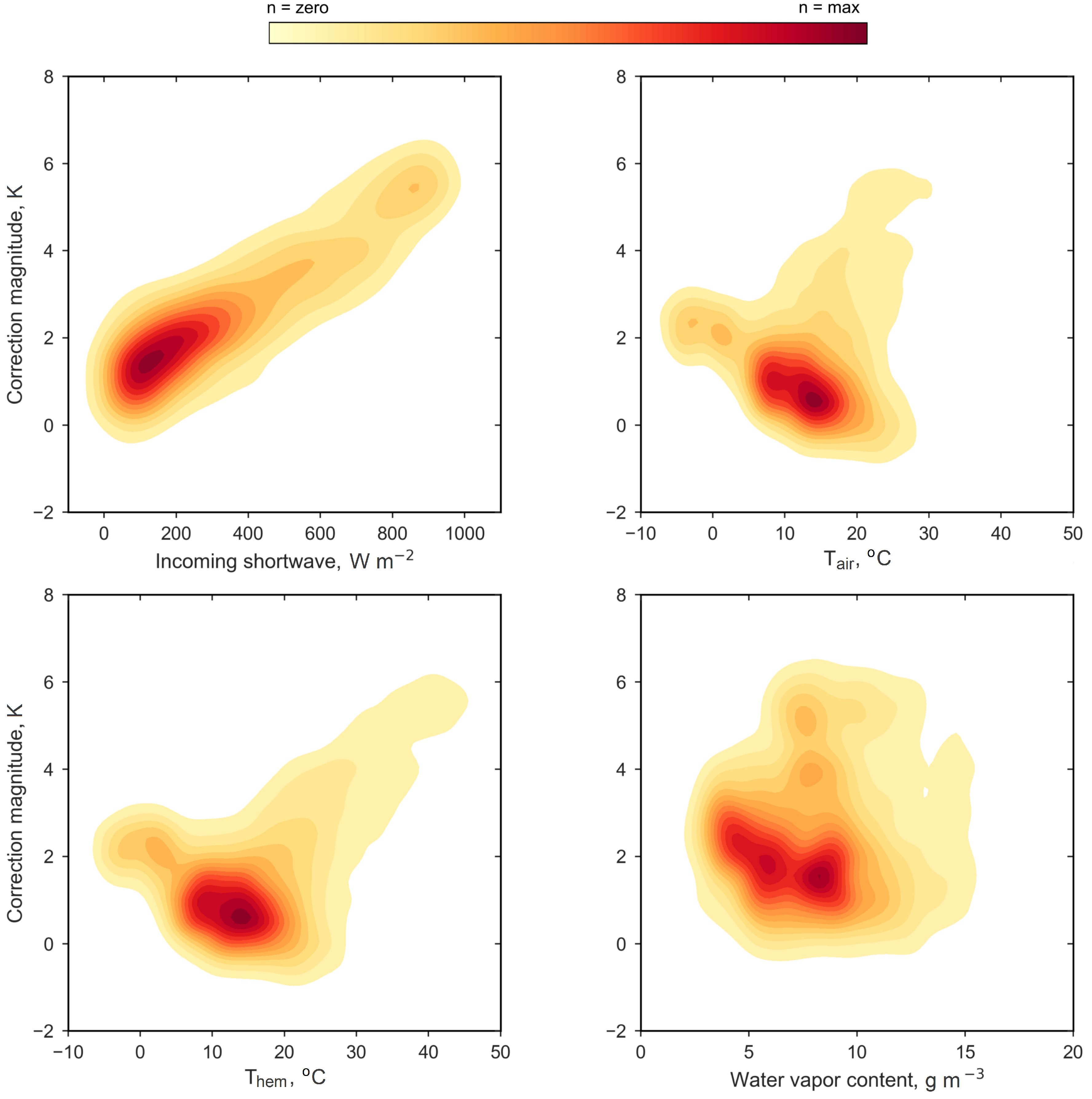
Figure 11.
Hemispherical at-sensor atmospheric transmittance as a function of water vapor content for two pyrgeometer heights (10 and 30 ) over a flat surface. Results calculated as the fraction of surface emission reaching the sensor height using MODTRAN 4.1 [15] with Tsurf = Tair = 300 , water vapor as the sole atmospheric absorber, and density and pressure from the Standard Atmosphere profile [25].

Figure 12.
A comparison of mean Them, r and Tplan normalized by Tcomp at 30 intervals from 26 June 2002 through 9 July 2002 during the intensive observation period. Shading indicates the area bounded by the first and third quartiles; n = 14 days.
Figure 12.
A comparison of mean Them, r and Tplan normalized by Tcomp at 30 intervals from 26 June 2002 through 9 July 2002 during the intensive observation period. Shading indicates the area bounded by the first and third quartiles; n = 14 days.
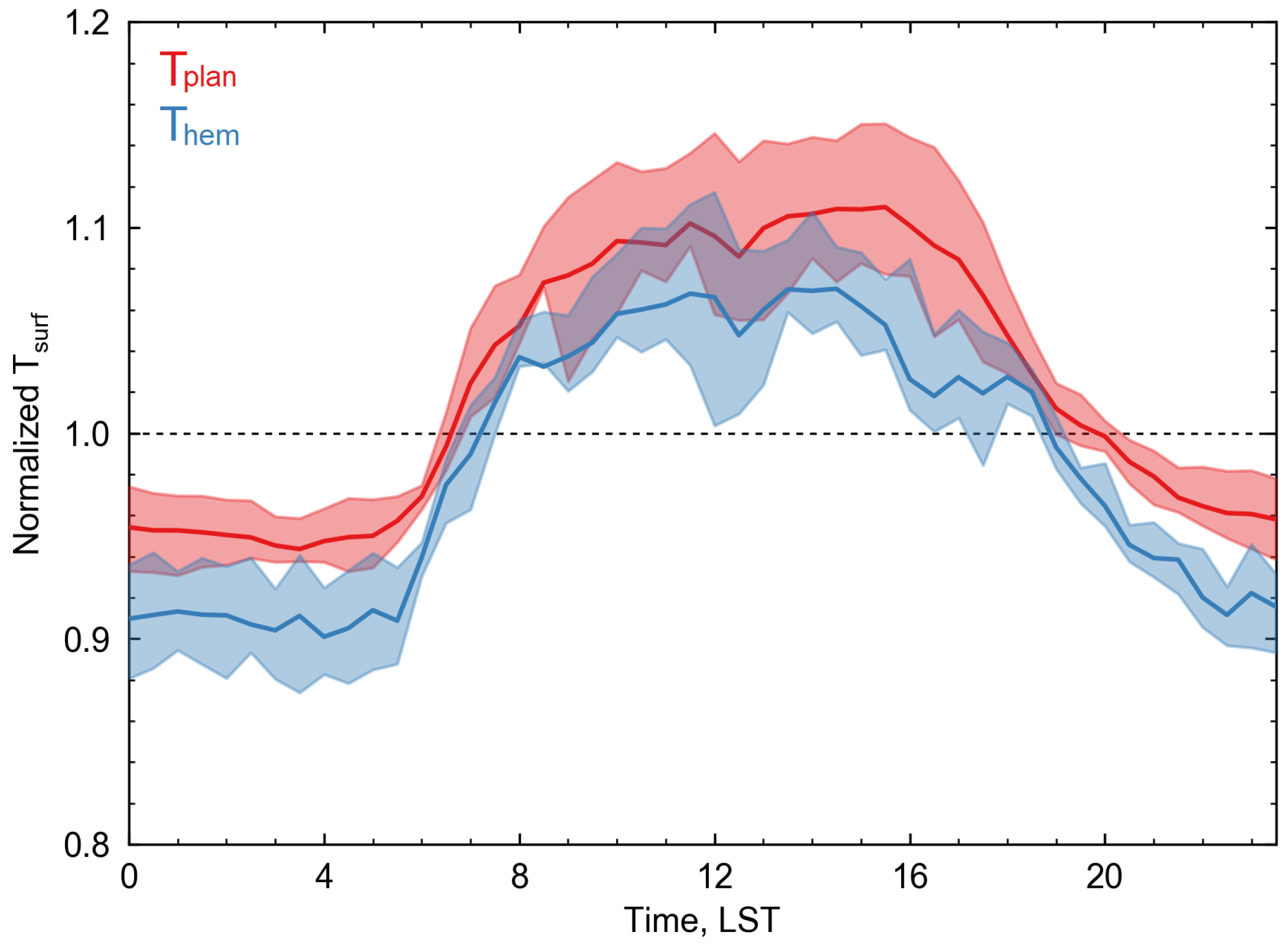
Figure 13.
Normalized Them, r, Tplan, and Tplan−hem, r averaged over 26 June 2002 through 9 July 2002 during the IOP and for clear sky and overcast days over the same period; n = 14 days.
Figure 13.
Normalized Them, r, Tplan, and Tplan−hem, r averaged over 26 June 2002 through 9 July 2002 during the IOP and for clear sky and overcast days over the same period; n = 14 days.
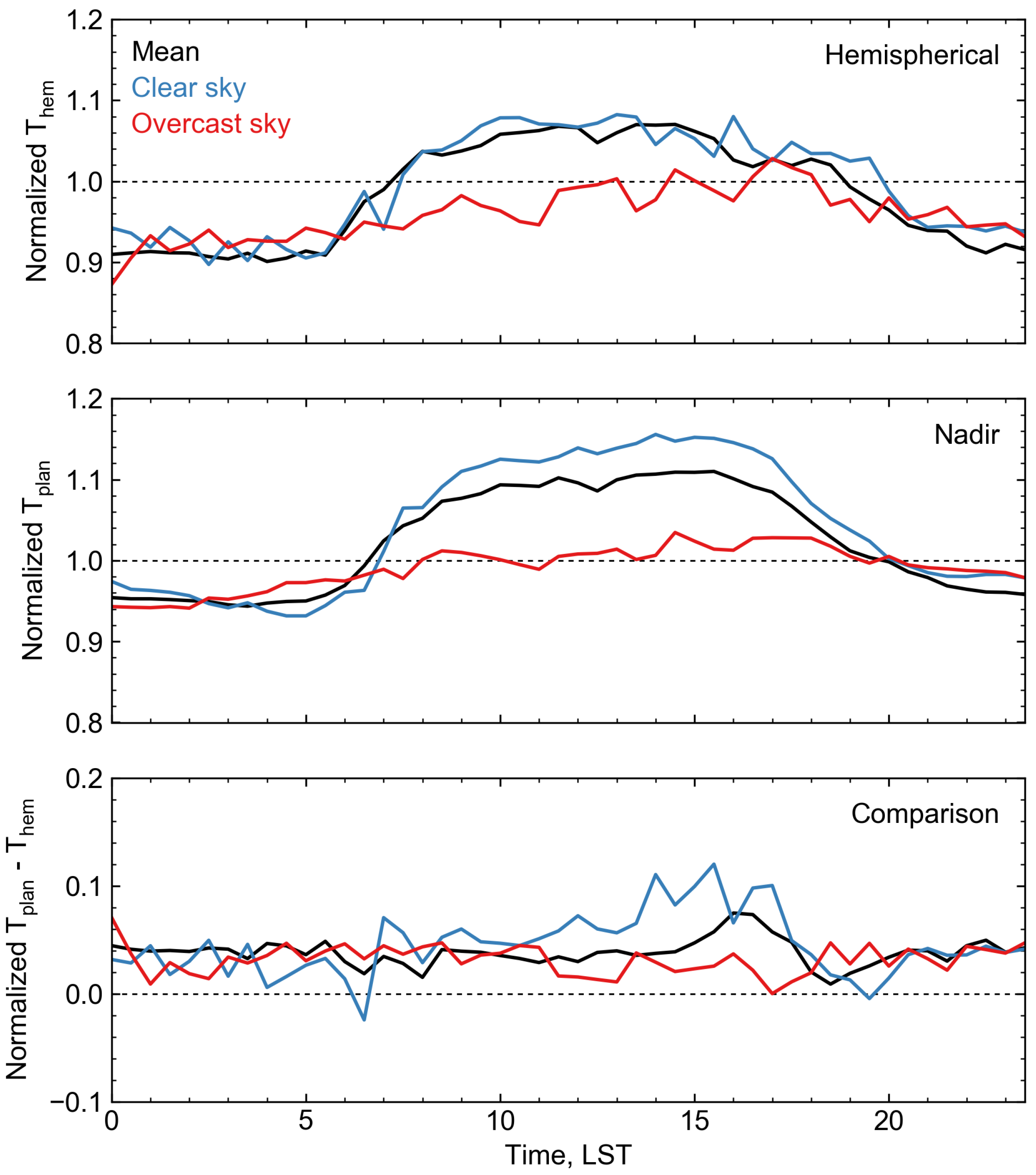
Figure 14.
Spectral dome transmittance for a Kipp and Zonen pyrgeometer overlaid with Planckian spectral radiance curves at T = 260 , 300 , and 320 . This illustrates the different relative effects of the pyrgeometer spectral dome transmittance on Planckian radiances at different temperatures.
Figure 14.
Spectral dome transmittance for a Kipp and Zonen pyrgeometer overlaid with Planckian spectral radiance curves at T = 260 , 300 , and 320 . This illustrates the different relative effects of the pyrgeometer spectral dome transmittance on Planckian radiances at different temperatures.

Table 1.
A description of morphological parameters and measured variables for the selected urban and rural sites from the Basel Urban Boundary Layer Experiment. Modified from Rotach et al. [13] to include only relevant parameters.
Table 1.
A description of morphological parameters and measured variables for the selected urban and rural sites from the Basel Urban Boundary Layer Experiment. Modified from Rotach et al. [13] to include only relevant parameters.
| Site | Location | Morphological | Meteorological Variables | Radiation |
|---|---|---|---|---|
| Height | Characteristics 1 | [No of Levels] 2 | [No of Levels] 3 | |
| Basel Sperrstrasse | 47.57 N | = 14.6 | Tair [7] | Lup [3] |
| Urban street canyon | 7.60 E | = 6.9 | H [7] | Ldown [5] |
| Local Climate Zone: 2 | 255 a.s.l. | H/W = 1.0 | WV [12] | Kup [2] |
| = 1.92 | WD [1] | Kup [2] | ||
| = 0.54 | P [1] | |||
| = 11.0% |
1 : average building height, : standard deviation of building height, : plan aspect ratio, : complete aspect ratio, H/W: local canyon height to width ratio, : surface albedo. 2 H: humidity, WV: wind velocity, WD: wind direction, P: pressure. 3 Lup: upwelling longwave radiation, Ldown: downwelling longwave radiation, Kup: upwelling shortwave radiation, Kdown: downwelling shortwave radiation.
Table 2.
Weights applied to individual wall, roof, and road surface temperature components in order to calculate complete and nadir temperatures for the Basel Sperrstrasse street canyon.
Table 2.
Weights applied to individual wall, roof, and road surface temperature components in order to calculate complete and nadir temperatures for the Basel Sperrstrasse street canyon.
| Road | NNW | SSE | NNW | SSE | |
|---|---|---|---|---|---|
| Roof | Roof | Wall | Wall | ||
| Complete (Tcomp) | 0.36 | 0.16 | 0.16 | 0.16 | 0.16 |
| Nadir (Tplan) | 0.46 | 0.27 | 0.27 | 0.00 | 0.00 |
Table 3.
Statistical performance of Them derived using the parameterization scheme relative to modeled Them,r. MAE is mean absolute error. RMSEs and RMSEu represent the systemic and unsystematic root-mean-square error, respectively. Statistical tests were selected from [29,30]; n = 853.
| Statistic | Parameterization |
|---|---|
| Slope | 1.058 |
| Intercept, () | −1.488 |
| R2 | 0.991 |
| MAE, () | 0.607 |
| RMSE, () | 0.757 |
| RMSEs, () | 0.476 |
| RMSEu, () | 0.588 |
| d, agreement index | 0.998 |
Table 4.
Statistical performance of the Payerne evaluation calculated at 30 intervals over a continuous 14-day period. MAE is mean absolute error. RMSEs and RMSEu represent the systemic and unsystematic root-mean-square error respectively. Statistical tests were selected from [29,30]; n = 378.
| Statistic | 10 m Flux | 30 m Flux | Divergence |
|---|---|---|---|
| Slope | 1.002 | 1.011 | 0.792 |
| Intercept, () | 0.422 | −3.560 | −0.583 |
| R2 | 0.995 | 0.996 | 0.863 |
| MAE, () | 1.781 | 1.325 | 1.191 |
| RMSE, () | 2.204 | 1.690 | 1.423 |
| RMSEs, () | 1.444 | 0.851 | 1.028 |
| RMSEu, () | 1.666 | 1.460 | 0.985 |
| d, agreement index | 0.999 | 0.999 | 0.959 |
Table 5.
Planck weighted mean spectral dome transmittance for a suite of common Tsurf.
| Temiss, | , % | Temiss, | , % |
|---|---|---|---|
| 260 | 48.3 | 295 | 49.6 |
| 265 | 48.5 | 300 | 49.7 |
| 270 | 48.7 | 305 | 50.0 |
| 275 | 48.9 | 310 | 50.1 |
| 280 | 49.1 | 315 | 50.3 |
| 285 | 49.3 | 320 | 50.4 |
| 290 | 49.4 |
© 2017 by the authors. Licensee MDPI, Basel, Switzerland. This article is an open access article distributed under the terms and conditions of the Creative Commons Attribution (CC BY) license (http://creativecommons.org/licenses/by/4.0/).
Share and Cite
MDPI and ACS Style
Allen, M.A.; Voogt, J.A.; Christen, A. Time-Continuous Hemispherical Urban Surface Temperatures. Remote Sens. 2018, 10, 3. https://doi.org/10.3390/rs10010003
AMA Style
Allen MA, Voogt JA, Christen A. Time-Continuous Hemispherical Urban Surface Temperatures. Remote Sensing. 2018; 10(1):3. https://doi.org/10.3390/rs10010003
Chicago/Turabian StyleAllen, Michael A., James A. Voogt, and Andreas Christen. 2018. "Time-Continuous Hemispherical Urban Surface Temperatures" Remote Sensing 10, no. 1: 3. https://doi.org/10.3390/rs10010003
Note that from the first issue of 2016, this journal uses article numbers instead of page numbers. See further details here.